Mass Spectrum of Heavy Quarkonium Hybrids

In the constituent quark model, hadrons are described as $q\bar{q}$ mesons and $qqq$ baryons. Most of the experimentally observed resonances can be accommodated in the quark model [1, 2]. However, QCD itself allows a much richer hadron spectrum, such as multiquarks, hybrids, glueballs, etc… [3]. Hybrid mesons ($\bar{q}gq$) are composed of a color-octet quark-antiquark pair and an excited gluonic field. Since the excited gluonic field could carry quantum numbers other than $0^{++}$, hybrids can appear with both the ordinary (the same as conventional $q\bar{q}$ mesons) and exotic quantum numbers ($J^{PC}=0^{--},0^{+-},1^{-+},2^{+-},\ldots$). The states with the exotic quantum numbers are not accessible for a $q\bar{q}$ state. Hybrids provide a good platform to search for these exotic quantum numbers.

The light hybrids were studied in the MIT bag model [4, 5], in which the hybrids with $J^{PC}=(0,1,2)^{-+},1^{--}$ were predicted to form the lightest hybrid supermultiplet consisting of a S-wave color-octet quark-antiquark pair coupled to an excited gluonic field with $J_{g}^{P_{g}C_{g}}=1^{+-}$. A higher hybrid supermultiplet composed of a P-wave $q\bar{q}$ pair and the same gluonic excitation would contain states with $J^{PC}=0^{+-},(1^{+-})^{3},(2^{+-})^{2},3^{+-},(0,1,2)^{++}$, where the superscript denotes the number of such states [6, 7]. Many other methods such as the flux tube model [8, 9, 10, 11, 12], lattice QCD [13, 14, 15, 16] and QCD sum rules [17, 18, 19, 20, 21, 22, 23, 24] were also used to study the light hybrids. To date, there is some evidence of the exotic light hybrid with $J^{PC}=1^{-+}$ [25, 26, 27, 28].

For heavy quarkonium hybrids, which hereafter we shall refer to as heavy quark hybrids, calculations including the constituent gluon model [29], the flux tube model [10], QCD sum rules [30, 31, 32, 33, 34, 35, 36] and lattice QCD [37, 38, 39, 40, 41, 6] have been performed. The hybrid supermultiplet structures described above were confirmed for the heavy quark sector in lattice QCD [6] and the P-wave quasigluon approach [42]. So far, however, no definitive experimental signal for heavy hybrid mesons has been observed, although many unexpected charmonium-like and bottomonium-like states have been discovered in the past several years [43, 44, 45, 46, 47]. Some of these states, called $X,\,Y,\,Z$, do not fit in the conventional quark model easily and are considered to be candidates for exotic states beyond the quark model, such as molecular states, tetraquarks, baryonium and quarkonium hybrids. For example, $Y(4260)$ was interpreted as a charmonium hybrid state in Refs. [48, 49, 3]. In Ref. [50], $X(3872)$ was also proposed to be a charmonium hybrid. To search for hybrids in the heavy quarkonium region further theoretical investigations of the hybrid spectrum are still needed.

QCD sum rules is a very powerful non-perturbative method [51, 52, 53] which has been widely used to study hadron structures. In Refs. [30, 31, 32], Govaerts et al. performed a QCD sum-rule analysis of the heavy quark hybrids including leading-order contributions up to the dimension four gluonic condensate. The sum rules of some $J^{PC}$ channels were unstable and thus these mass predictions were unreliable. Recently, the $J^{PC}=1^{--}$ [34], $1^{++}$ [35] and $0^{-+}$ [36] channels have been re-analyzed by including the dimension six tri-gluon condensate. The dimension six contributions have proven to be very important because they stabilize the hybrid sum rules and allow mass prediction to be made. In this work, we will study the mass spectrum of heavy quarkonium hybrids using the QCD sum rule method. We will calculate the dimension six condensates including $\langle g_{s}^{3}fGGG\rangle$ and the light-quark condensate $\langle g_{s}^{4}jj\rangle$, where the latter condensate has not previously been calculated in the hybrid sum rules.

The paper is organized as follows. In Sec. II, we calculate the correlation functions and spectral densities of the hybrid operators with various quantum numbers and collect them in Appendix A. In Sec. III, we perform the numerical analysis and extract masses of charmonium and bottomonium hybrids. In the last section we summarize our results and comment on their implications for heavy quarkonium spectroscopy.

We consider the two-point correlation function

where $J_{\mu}$ is the interpolating current. In this work, we use the following hybrid interpolating currents coupling to various quantum numbers:

in which $Q$ represents a heavy quark ($c$ or $b$), $g_{s}$ is the strong coupling, $\lambda^{a}$ are the Gell-Mann matrices and $G^{a}_{\mu\nu}$ is the gluon field strength. By replacing $G^{a}_{\mu\nu}$ with $\tilde{G}^{a}_{\mu\nu}=\frac{1}{2}\epsilon_{\mu\nu\alpha\beta}G^{\alpha\beta,a}$, we can also obtain the corresponding operators with opposite parity. These hybrid correlation functions were originally studied in Refs. [30, 31, 32] in which the perturbative and gluon condensate contributions have been calculated to perform the QCD sum rule analysis. According to these calculations, the stability of the sum rules depends on the relative sign of the gluon condensate and the perturbative term. Only a relative negative sign results in stable sum rules. As shown in Refs. [30, 31, 32], the sum rules for $J^{PC}=0^{--},0^{++},1^{+-},1^{++},2^{++}$ channels are stable while the $J^{PC}=0^{-+},0^{+-},1^{-+},1^{--},2^{-+}$ channels are unstable. In this work, we will calculate the dimension six condensates in the correlation functions and show that they stabilize the hybrid sum rules for all unstable $J^{PC}=0^{-+},0^{+-},1^{-+},1^{--},2^{-+}$ channels, confirming the stabilizing effect of dimension six condensates previously found for $1^{--}$ [34], $1^{++}$ [35] and $0^{-+}$ [36].

For the hybrid operators in Eq. (2), the two-point correlation functions have the following structures:

where $\eta_{\mu\nu}=q_{\mu}q_{\nu}/q^{2}-g_{\mu\nu}$. $\Pi_{V}(q^{2})$, $\Pi_{S}(q^{2})$ in Eq. (3) and $\Pi_{T}(q^{2})$ in Eq. (4) are the invariant structures referring to pure spin-1, spin-0 and spin-2 states, respectively. In Eq. (4), the invariant structures for spin-0 and spin-1 are not written out explicitly because we will not consider contributions arising from these terms in this paper.

At the hadron level, the correlation function can be described by the dispersion relation,

The summation on the right hand side represents the subtraction terms which can be removed by taking the Borel transform of $\Pi(q^{2})$. The spectral function $\rho(s)$ is defined using the pole plus continuum approximation

where the intermediate states $n$ must have the same quantum numbers as the interpolating currents $J_{\mu}$, $m_{X}$ denotes the mass of the lowest lying resonance and the dimensionless quantity $f_{X}$ is the coupling of the resonance to the current

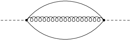
At the quark-gluon level, the correlation function can be computed via the operator product expansion (OPE). For heavy quark hybrids, the quark condensates are expressed in terms of the gluon condensate via the heavy quark mass expansion and hence give no contributions to the correlation function. To calculate the correlation function, only the perturbative diagram (Fig. 1), gluon condensate diagram (Fig. 2) and diagrams for dimension six condensates (Fig. 3) are involved. In Fig 3, the dimension six condensates contain $\langle g_{s}^{3}fGGG\rangle$ (Fig. 3b) and $\langle DDG\rangle$ (Fig. 3a). Using the equation of motion, Bianchi identities and commutation relations, the condensate $\langle DDG\rangle$ can be expressed in terms of $\langle g_{s}^{3}fGGG\rangle$ and $\langle g_{s}^{4}jj\rangle$.

We have calculated the Wilson coefficients using two independent techniques, finding complete agreement between them. First, we have used the same approach that was utilized in Refs. [35, 36] for $0^{-+}$ and $1^{++}$ heavy hybrids, respectively. In this approach, we utilize the Mathematica package Tarcer [54], which implements the $d$ dimensional recurrence relations developed in Refs. [55, 56] to reduce the number of distinct integrals that must be calculated. The resulting minimal set of loop integrals can be evaluated using results given in Refs. [57, 58, 59], leading to very compact expressions for the Wilson coefficients in terms of generalized hypergeometric functions. Second, we have utilized the technique used in Refs. [60, 61, 62, 63]. With this method the perturbative spectral densities are expressed as integrations that can be performed numerically. In this approach we use the momentum space quark propagator

where $\sigma^{\mu\nu}=\frac{i}{2}\left[\gamma^{\mu}\,,\gamma^{\nu}\right]$, and $a\,,b$ are color indices. To our knowledge, this is the first time that these two calculational approaches have been directly compared, therefore the agreement between them is noteworthy. In addition, we interpret this agreement as a very robust test of the veracity of our results.

The correlation function obtained at the quark-gluon level should be equivalent to that described at the hadron level due to quark-hadron duality, establishing a sum rule to extract the hadron mass. The Borel transform is applied to the correlation functions at both levels to pick out the lowest lying resonance, eliminate dispersion-relation subtractions, and enhance the OPE convergence. Using the spectral function in Eq. (6), we arrive at

where $s_{0}$ is the continuum threshold parameter and $M_{B}$ is the Borel mass. Then the hadron mass can be extracted using

in which $m_{X}$ denotes the heavy hybrid mass.

For all the interpolating currents in Eq. (2), we calculate the correlation functions and the spectral densities are then obtained via $\rho(s)=\frac{1}{\pi}$Im$\Pi(s)$. We list the expressions for the correlation functions and the spectral densities in Appendix A. As mentioned above, we have used two distinct methods to determine these expressions for the spectral functions. First, we have used the same method as in Refs. [35, 36] to calculate the full correlation function, from which the imaginary part can be extracted through analytic continuation and hence a closed form expression for the spectral function can be constructed. Second, we have used the method of Refs. [60, 61, 62, 63] which can be used to determine integral representations of the spectral functions. We have numerically verified that these two approaches lead to identical results. This provides a very strong test of our results. Another check is that our results for the perturbative and gluon condensate contributions are in numerical agreement with those in Refs. [30, 31, 32].

Besides the perturbative term and the dimension four gluon condensate $\langle\alpha_{s}GG\rangle$, we also calculate the dimension six condensates $\langle g_{s}^{3}fGGG\rangle$ and $\langle g_{s}^{4}jj\rangle$. The condensate $\langle g_{s}^{4}jj\rangle$ has not previously been evaluated in the hybrid sum rules. As mentioned above, it comes from applying equations of motion in the condensate $\langle DDG\rangle$ arising from the diagram Fig. (3a). Within the vacuum factorization assumption, $\langle g_{s}^{4}jj\rangle$ is proportional to the square of $g_{s}^{2}\langle\bar{q}q\rangle$. Although the numerical analysis shows that $\langle g_{s}^{4}jj\rangle$ is small enough to be ignored compared to $\langle g_{s}^{3}fGGG\rangle$, we include its contribution in our analysis because of the important stabilizing role of the dimension six condensates. We have only included the integral representations for these contributions in Appendix A.

From the formulae for the spectral densities in Appendix A, we find that the perturbative contributions are invariant and the gluon condensate and tri-gluon condensate contributions change sign under parity reversal. This is in agreement with the results for the perturbative and gluon condensate contributions in Refs. [30, 31, 32]. It should be noted that both the expression for $\rho^{\langle GGG\rangle}$ and that of $\rho^{\langle jj\rangle}$ have a singularity at $s=4m^{2}$. One should be very cautious in calculating the Borel transforms of the correlation functions from these expressions due to these singularities. In Refs. [35, 36] a numerical limiting procedure was developed based on the full analytic structure of the correlation functions and the relation between the Borel transform and inverse Laplace transform. This limiting procedure serves to cancel the integration divergences at $s=4m^{2}$ in the $\eta\to 0$ limit. A suitable value of $\eta$ should be determined to perform the numerical analysis. Alternatively, these divergences can also be eliminated if we use the integral forms of $\rho^{\langle GGG\rangle}$ and $\rho^{\langle jj\rangle}$ in Eqs. (26)–(35) where the delta functions absorb divergences of the spectral densities at $x=0$ and $x=1$. The $\eta\to 0$ limiting expressions are necessary when the closed form expressions for the spectral densities are used (see Appendix A).

To perform the QCD sum rule numerical analysis, we use the following values of the heavy quark masses and the condensates [64, 65, 66, 67]:

in which the charm and bottom quark masses are the running masses in the $\overline{\rm MS}$ scheme. Note that there is a minus sign implicitly included in the definition of the coupling constant $g_{s}$ in this work. We choose the renormalization scale $\mu=\overline{m}_{c}$ for the charmonium systems and $\mu=\overline{m}_{b}$ for bottomonium systems, but other choices of renormalization scale for the $\overline{\rm MS}$ masses can be expressed via the leading order expressions:

For the hybrid charmonium and bottomonium analyses, the strong coupling is then determined by evolution from the $\tau$ and $Z$ masses, respectively:

in which the $\tau$ and $Z$ masses, $\alpha_{s}(M_{\tau})$ and $\alpha_{s}(M_{Z})$ are from the Particle Data Group [2]. Apart from small chiral-violating effects, the QCD condensate $\langle\alpha_{s}GG\rangle$ is renormalization scale invariant. Although $\langle g_{s}^{4}jj\rangle$ has complicated renormalization-group behaviour [68], these effects are negligible because the contribution from this condensate is a small numerical effect. Finally, the condensate $\langle g_{s}^{3}fGGG\rangle$ in (12) is determined at the scale $\mu=\overline{m}_{c}$ [65] so our charmonium analysis is self-consistent and does not require renormalization-group evolution of $\langle g_{s}^{3}fGGG\rangle$. For bottomonium systems, the effect of the $\langle g_{s}^{3}fGGG\rangle$ anomalous dimension [68] has been found to be negligible [69].

We begin with the sum-rule analysis of the hybrid charmonium mass spectrum. The stability of the QCD sum rule requires suitable working regions for the continuum threshold parameter $s_{0}$ and Borel mass $M_{B}$. According to Eq. (10), excited state contributions are naturally suppressed by the exponential weight function for small $M_{B}^{2}$. The lowest lying resonance contribution will be enhanced in the same region. On the other hand, however, the OPE convergence suffers if $M_{B}^{2}$ is too small. In our analysis, the Borel mass working region is determined by the convergence of the OPE series and the pole contribution. The requirement of OPE convergence determines the lower bound on $M_{B}^{2}$ while the pole contribution constraint leads to the upper bound.

For hybrid charmonium the dominant nonperturbative contributions come from the gluon condensate $\langle\alpha_{s}GG\rangle$. However, the dimension six condensates are also important because they can stabilize the mass sum rules [34, 36, 35]. We have calculated dimension six condensates $\langle g_{s}^{3}fGGG\rangle$ and $\langle g_{s}^{4}jj\rangle$ in the spectral densities, extending the results of [30, 31, 32]. From the numerical analysis, we see that the condensate $\langle g_{s}^{4}jj\rangle$ is much smaller than $\langle g_{s}^{3}fGGG\rangle$ (Fig. III). To study the OPE convergence, we require that the gluon condensate be less than one third of the perturbative term while the tri-gluon condensate be less than one third of the gluon condensate. This requirement gives the lower bound on $M_{B}^{2}$. For example, we show the OPE convergence for the exotic channel $J^{PC}=1^{-+}$ in Fig. III, from which we obtain the lower bound of the Borel mass $M_{Bmin}^{2}=4.6$ GeV².

We define the pole contribution (PC) as:

where PC is a function of $s_{0}$ and $M_{B}^{2}$. In order to study its dependence on $M_{B}^{2}$, one should first fix the value of $s_{0}$. In order to do so we study the variation of the hybrid mass $m_{X}$ versus $s_{0}$, as shown in Fig. III for the $J^{PC}=1^{-+}$ channel. We find that the hybrid mass is very stable for different values of $M_{B}^{2}$ around $s_{0}=17$ GeV². Using this value of $s_{0}$, we obtain the upper bound on the Borel mass of $M_{\rm Bmax}^{2}=6.5$ GeV² by requiring the pole contribution be larger than $10\%$ in Eq. (17). In Fig. III, we plot the Borel curve of $m_{X}$ versus $M_{B}^{2}$ for the $1^{-+}$ charmonium hybrid, which shows that the mass sum rule is very stable in the $M_{B}^{2}$ working region. Finally, the predicted mass of the exotic $J^{PC}=1^{-+}$ hybrid charmonium is $3.70$ GeV. This value is about $0.5$ GeV lower than the lattice result in Ref. [6].

After performing the QCD sum rule analyses, we extract masses of the charmonium hybrids with various quantum numbers as summarized in Table III. We also give the corresponding Borel windows, threshold values and pole contributions. Only errors from the uncertainties in the charm quark mass and the condensates are taken into account. We do not consider other possible error sources such as truncation of the OPE series, the uncertainty of the threshold value $s_{0}$ and the variation of Borel mass $M_{B}$. In fact, the dominant error is from the uncertainty of the gluon condensate for the channels with $J^{PC}=0^{--},0^{++},1^{++},1^{+-},2^{++}$ while the tri-gluon condensate dominates for those with $J^{PC}=0^{-+},0^{+-},1^{-+},1^{--},2^{-+}$. The errors from the charm quark mass $m_{c}$ and $\langle g_{s}^{4}jj\rangle$ are much smaller.

The results show that for the unstable channels with $J^{PC}=0^{-+},0^{+-},1^{-+},1^{--},2^{-+}$ in Refs. [30, 31, 32], the dimension six condensate $\langle g_{s}^{3}fGGG\rangle$ in the spectral functions can stabilize the systems and make it possible to extract the hybrid masses. This universal trend confirms the stabilizing effect of dimension six condensates previously observed for the $J^{PC}=1^{--}$ [34], $1^{++}$ [35] and $0^{-+}$ [36] channels. For these previously unstable channels, the pole contributions are very small even though we consider the dimension six condensates contributions. The small pole contributions result in the narrow Borel windows compared to the stable channels in Refs. [30, 31, 32] with $J^{PC}=0^{--},0^{++},1^{++},1^{+-},2^{++}$. The $1^{++}$ and $0^{-+}$ results agree with the previous sum-rule analyses including the dimension six gluon condensates [36, 35]. However, the $1^{--}$ mass is somewhat smaller than in Ref. [34] a result we attribute to the absence of the QCD continuum from the condensates in Ref. [34]. We obtain four charmonium hybrid states with $J^{PC}=(0,1,2)^{-+},1^{--}$ in the range $3.4\sim 3.9$ GeV which are much lower than the other channels in Table III. However, the $1^{--}$ channel was examined in Ref. [70], finding a mass of 3.66 GeV, which is comparable to our prediction for this channel. In the MIT bag model [4, 5], the light hybrids with these quantum numbers have been predicted to form the lightest hybrid supermultiplet consisting of a S-wave color-octet $q\bar{q}$ pair coupled to a $J_{g}^{P_{g}C_{g}}=1^{+-}$ gluonic excitation. This supermultiplet was confirmed in the heavy quark sector using lattice QCD [6] and the P-wave quasigluon approach [42]. Our result supports this prediction although the extracted masses are $0.4\sim 0.7$ GeV lower. A heavier hybrid supermultiplet in Refs. [6, 42] contains states with $J^{PC}=0^{+-},(1^{+-})^{3},(2^{+-})^{2},3^{+-},(0,1,2)^{++}$. It is composed of a P-wave color-octet $q\bar{q}$ pair coupled to a gluonic field with $J_{g}^{P_{g}C_{g}}=1^{+-}$. In Table III, we list our mass predictions for the $J^{PC}=(0,1)^{+-},(0,1,2)^{++}$ members of this excited hybrid supermultiplet.

We obtain three charmonium hybrid states with exotic quantum numbers $J^{PC}=1^{-+},0^{+-},0^{--}$ in Table III. The experimental identification of these states is considered to be a smoking gun for the existence of the gluonic degree of freedom in QCD because they cannot mix with the conventional charmonium states. The lightest exotic charmonium hybrid state with $J^{PC}=1^{-+}$ in the first hybrid supermultiplet is particularly important. The mass of the heaviest hybrid charmonium with $J^{PC}=0^{--}$ is about $5.5$ GeV, which is consistent with the lattice QCD prediction [39] within the errors. This large mass may suggest that it has highly excited gluonic structures.

In principle, conventional charmonium $c\bar{c}$ states can also couple to the charmonium hybrid currents with the same quantum numbers. Although a full analysis of the mixed hybrid/charmonium scenario is beyond the scope of this work (see e.g., Ref. [70]) we can explore the qualitative effect of mixing on our mass predictions by modifying the right-hand side of (10) to include a conventional charmonium ground state $m_{c\bar{c}}$

so that (11) becomes

By inputting the known charmonium mass $m_{c\bar{c}}$ and allowing $f_{c}$ to increase from zero (i.e. the pure hybrid case) we can determine how the hybrid mass is influenced by mixing. Fig. III shows that the $1^{--}$ hybrid state mass increases as mixing with conventional charmonium increases and similar behaviour is found for all the other non-exotic cases. Mixing effects will thus tend to raise the mass predictions of Table III implying that our results are a lower bound on the mixed hybrid mass. A conservative estimate would be a mixed mass in the upper range of the uncertainties given in Table III.

The quantum numbers of $X(3872)$ are given as $J^{PC}=1^{++}$ or $2^{-+}$ in the PDG  [2]. Although the analysis of angular distributions favors the assignment $J^{PC}=1^{++}$ [71, 72], the $2^{-+}$ assignment is also possible [73]. Recently, the LHCb collaboration has provided strong evidence for $J^{PC}=1^{++}$ [74]. As previously found in Ref. [35], the mass of the $1^{++}$ hybrid charmonium in Table III is around $5.06$ GeV, which is much higher than the mass of $X(3872)$, which seems to preclude a pure hybrid interpretation as pointed out in Ref. [35]. The mass of the $2^{-+}$ hybrid charmonium is about $4.45$ GeV, which also precludes the $2^{-+}$ hybrid charmonium assignment for the $X(3872)$, in agreement with the LHCb result [74].

By replacing $m_{c}$ with $m_{b}$ in the spectral densities and using the strong coupling in Eq. (16), we perform the same analysis as described above and collect the numerical results for bottomonium hybrid states in Table III. Obviously the Borel windows are enlarged compared to the hybrid charmonium systems, which means that the stabilities are better for the bottomonium hybrid states. We show the Borel curves of the bottomonium hybrid state with $J^{PC}=1^{-+}$ in Fig. III. In Table III, the masses of the four bottomonium hybrid states with $J^{PC}=(0,1,2)^{-+},1^{--}$ are about $9.7\sim 9.9$ GeV. The mass variations of these states are much smaller than those in the charmonium system. They form the lightest bottomonium supermultiplet, in complete analogy with the charmonium hybrid supermultiplet structure. In Table III, the masses of $0^{-+}$ and $1^{++}$ bottomonium hybrids are again in agreement with Refs. [36, 35] and the $0^{--}$ state is still the heaviest one.

In this paper we have studied the mass spectrum of charmonium and bottomonium hybrids using QCD sum rules. Using the hybrid operators in Eq. (2), we calculate the correlation functions and the spectral densities, confirming the perturbative and gluon condensate results of [30, 31, 32] and extending them to include the dimension six condensates $\langle g_{s}^{3}fGGG\rangle$ and $\langle g_{s}^{4}jj\rangle$. Agreement with the $\langle g_{s}^{3}fGGG\rangle$ results of Refs. [36, 35] provides an additional consistency check on our analysis. Expressions for the correlation functions and spectral densities are given in Appendix A.

The Feynman diagram in Fig. (3a) gives contributions to both the condensates $\langle g_{s}^{3}fGGG\rangle$ and $\langle g_{s}^{4}jj\rangle$. The condensate $\langle g_{s}^{4}jj\rangle$ has not previously been calculated in hybrid sum rules. Given the crucial stabilizing contribution of the dimension six gluon condensate, we have also included the dimension six quark condensate in our analysis. The channels with $J^{PC}=0^{-+},0^{+-},1^{-+},1^{--},2^{-+}$ were unstable without the contributions of the dimension six condensates in the original QCD sum rule analysis [30, 31, 32]. However, these channels are stabilized by the effects of the dimension six condensates in our analysis. In our analysis all channels lead to stable mass sum rules. Due to the small values of the pole contribution, the Borel windows of the channels with $J^{PC}=0^{-+},0^{+-},1^{-+},1^{--},2^{-+}$ are much narrower than those of $J^{PC}=0^{--},0^{++},1^{++},1^{+-},2^{++}$. We speculate that this explains why these channels were unstable in Refs. [30, 31, 32]; the pole contributions were so small that no effective working regions for Borel parameter existed. Although the $\langle g_{s}^{4}jj\rangle$ effects are very small compared to $\langle g_{s}^{3}fGGG\rangle$, we still include its contribution to the correlation function in this work because of the important stabilizing role of the dimension six condensates.

The sum-rule mass predictions show that for the charmonium hybrids, there are four negative-parity states with $J^{PC}=(0,1,2)^{-+},1^{--}$ which lie below 4 GeV. Their masses are about $3.4\sim 3.9$ GeV and are much lower than the other states, forming the lightest charmonium hybrid supermultiplet. Our mass prediction for the $1^{--}$ state is comparable to the result found in Ref. [70], which provides indirect support for our mass predictions for the states in the lightest supermultiplet. These states were predicted to form the lightest hybrid supermultiplet in lattice QCD [6] and the P-wave quasigluon approach [42], consisting of a S-wave color-octet $q\bar{q}$ pair and a $1^{+-}$ excited gluonic field. A heavier hybrid supermultiplet is composed of a P-wave color-octet $q\bar{q}$ pair coupled to a $1^{+-}$ excited gluonic field [6, 42]. In our spectrum, we predict masses of five positive-parity members of this excited hybrid supermultiplet with $J^{PC}=(0,1)^{+-},(0,1,2)^{++}$. We speculate that the supermultiplets are occupied by states of the same parity because of the behaviour of the perturbative, gluon condensate and dimension six condensate contributions under parity reversal. In particular, Appendix A shows that the perturbative contributions are invariant and the gluon condensate and tri-gluon condensate contributions change sign under parity reversal, implying a consistent pattern in the mass hierarchy of the positive- and negative-parity states. We note that the $J^{PC}=0^{--}$ hybrid has a much higher mass in our spectrum which may suggest that it involves a different excitation of the gluonic field compare to other channels. We list the masses of the charmonium and bottomonium hybrid states in Table III and Table III, respectively. Finally, we have investigated the effects of mixing between non-exotic hybrids and conventional quarkonia. We find that mixing increases the mass predictions for the non-exotic hybrids given in Tables III and III, and we conservatively estimate that the mixed states masses are in the upper range of the uncertainties given in Tables III and III. A more detailed study of mixing between non-exotic hybrids and conventional quarkonia is left for future work.

To date, there are many interpretations of the $X(3872)$ meson, such as a molecular state, a tetraquark state, and a charmonium hybrid. LHCb has provided strong evidence for the $J^{PC}=1^{++}$ quantum numbers, seemingly ruling out the $2^{-+}$ assignment [74]. In our spectrum, the masses of the $1^{++}$ and $2^{-+}$ charmonium hybrids are about $5.06$ GeV and $4.45$ GeV, respectively. The $1^{++}$ (also see Ref. [35]) and $2^{-+}$ mass predictions seem to preclude a pure charmonium hybrid interpretation of the $X(3872)$ meson.

Observation of the overpopulation of the states with $q\bar{q}$ quantum numbers in the charmonium and bottomonium regions, such as the $X,Y,Z$ states, is an important signal for the existence of the heavy quark hybrids. As an experimental signal, this overpopulation complements the identification of states with exotic quantum numbers. Experiments such as BESIII, PANDA and LHCb will collect more definitive data on the charmonium spectrum, including hybrid mesons. Our results for the mass spectra of charmonium and bottomonium hybrids in Table III and Table III may be useful for the future search for these fascinating exotic and non-exotic hybrid states at these experimental facilities.

This project was supported by the Natural Sciences and Engineering Research Council of Canada (NSERC). S.L.Z. was supported by the National Natural Science Foundation of China under Grants 11075004, 11021092, 11261130311 and Ministry of Science and Technology of China (2009CB825200).

References

• [1] S. Godfrey and N. Isgur, Phys.Rev. D32, 189 (1985).
• [2] J. Beringer et al. (Particle Data Group), Phys.Rev. D86, 010001 (2012).
• [3] E. Klempt and A. Zaitsev, Phys. Rept. 454, 1 (2007).
• [4] T. Barnes, F. Close, F. de Viron, and J. Weyers, Nucl.Phys. B224, 241 (1983).
• [5] M. S. Chanowitz and S. R. Sharpe, Nucl. Phys. B222, 211 (1983).
• [6] L. Liu et al. (Hadron Spectrum Collaboration), JHEP 1207, 126 (2012).
• [7] J. J. Dudek, Phys.Rev. D84, 074023 (2011).
• [8] N. Isgur, R. Kokoski, and J. E. Paton, Phys.Rev.Lett. 54, 869 (1985).
• [9] F. E. Close and P. R. Page, Phys.Rev. D52, 1706 (1995a), eprint hep-ph/9412301.
• [10] T. Barnes, F. E. Close, and E. S. Swanson, Phys. Rev. D52, 5242 (1995), eprint hep-ph/9501405.
• [11] P. R. Page, E. S. Swanson, and A. P. Szczepaniak, Phys. Rev. D59, 034016 (1999), eprint hep-ph/9808346.
• [12] F. E. Close and P. R. Page, Nucl.Phys. B443, 233 (1995b), eprint hep-ph/9411301.
• [13] C. McNeile, C. W. Bernard, T. A. DeGrand, C. E. DeTar, S. A. Gottlieb, et al., Nucl.Phys.Proc.Suppl. 73, 264 (1999).
• [14] P. Lacock and K. Schilling (TXL), Nucl. Phys. Proc. Suppl. 73, 261 (1999), eprint hep-lat/9809022.
• [15] C. Bernard, T. Burch, E. Gregory, D. Toussaint, C. E. DeTar, et al., Phys.Rev. D68, 074505 (2003), eprint hep-lat/0301024.
• [16] J. Hedditch, W. Kamleh, B. Lasscock, D. Leinweber, A. Williams, et al., Phys.Rev. D72, 114507 (2005), eprint hep-lat/0509106.
• [17] J. Govaerts, F. de Viron, D. Gusbin, and J. Weyers, Phys.Lett. B128, 262 (1983).
• [18] J. Govaerts, F. de Viron, D. Gusbin, and J. Weyers, Nucl. Phys. B248, 1 (1984).
• [19] J. Latorre, S. Narison, P. Pascual, and R. Tarrach, Phys.Lett. B147, 169 (1984).
• [20] J. I. Latorre, P. Pascual, and S. Narison, Z. Phys. C34, 347 (1987).
• [21] I. Balitsky, D. Diakonov, and A. Yung, Z.Phys. C33, 265 (1986).
• [22] H. Jin, J. Korner, and T. G. Steele, Phys.Rev. D67, 014025 (2003), eprint hep-ph/0211304.
• [23] K. G. Chetyrkin and S. Narison, Phys.Lett. B485, 145 (2000), eprint hep-ph/0003151.
• [24] S.-L. Zhu, Phys.Rev. D60, 097502 (1999a), eprint hep-ph/9903537.
• [25] D. Thompson et al. (E852 Collaboration), Phys.Rev.Lett. 79, 1630 (1997), eprint hep-ex/9705011.
• [26] A. Abele et al. (Crystal Barrel), Phys. Lett. B423, 175 (1998).
• [27] A. Abele et al. (Crystal Barrel), Phys. Lett. B446, 349 (1999).
• [28] G. S. Adams et al. (E862), Phys. Lett. B657, 27 (2007), eprint hep-ex/0612062.
• [29] D. Horn and J. Mandula, Phys.Rev. D17, 898 (1978).
• [30] J. Govaerts, L. J. Reinders, H. R. Rubinstein, and J. Weyers, Nucl. Phys. B258, 215 (1985a).
• [31] J. Govaerts, L. J. Reinders, and J. Weyers, Nucl. Phys. B262, 575 (1985b).
• [32] J. Govaerts, L. J. Reinders, P. Francken, X. Gonze, and J. Weyers, Nucl. Phys. B284, 674 (1987).
• [33] S.-L. Zhu, Phys. Rev. D60, 031501 (1999b), eprint hep-ph/9812469.
• [34] C.-F. Qiao, L. Tang, G. Hao, and X.-Q. Li, J.Phys. G39, 015005 (2012).
• [35] D. Harnett, R. T. Kleiv, T. G. Steele, and H.-y. Jin, J.Phys. G39, 125003 (2012).
• [36] R. Berg, D. Harnett, R. T. Kleiv, and T. G. Steele, Phys.Rev. D86, 034002 (2012).
• [37] S. Perantonis and C. Michael, Nucl.Phys. B347, 854 (1990).
• [38] K. J. Juge, J. Kuti, and C. J. Morningstar, Phys. Rev. Lett. 82, 4400 (1999), eprint hep-ph/9902336.
• [39] Y. Liu and X.-Q. Luo, Phys.Rev. D73, 054510 (2006), eprint hep-lat/0511015.
• [40] X.-Q. Luo and Y. Liu, Phys.Rev. D74, 034502 (2006), eprint hep-lat/0512044.
• [41] L. Liu, S. M. Ryan, M. Peardon, G. Moir, and P. Vilaseca, PoS LATTICE2011, 140 (2011).
• [42] P. Guo, A. P. Szczepaniak, G. Galata, A. Vassallo, and E. Santopinto, Phys.Rev. D78, 056003 (2008).
• [43] N. Brambilla, S. Eidelman, B. Heltsley, R. Vogt, G. Bodwin, et al., Eur.Phys.J. C71, 1534 (2011).
• [44] M. Nielsen, F. S. Navarra, and S. H. Lee, Phys. Rept. 497, 41 (2010).
• [45] E. S. Swanson, Phys. Rept. 429, 243 (2006), eprint hep-ph/0601110.
• [46] S.-L. Zhu, Int. J. Mod. Phys. E17, 283 (2008), eprint hep-ph/0703225.
• [47] J. L. Rosner, J. Phys. Conf. Ser. 69, 012002 (2007), eprint hep-ph/0612332.
• [48] S.-L. Zhu, Phys. Lett. B625, 212 (2005), eprint hep-ph/0507025.
• [49] F. E. Close and P. R. Page, Phys. Lett. B628, 215 (2005), eprint hep-ph/0507199.
• [50] F. E. Close and S. Godfrey, Phys. Lett. B574, 210 (2003), eprint hep-ph/0305285.
• [51] M. A. Shifman, A. I. Vainshtein, and V. I. Zakharov, Nucl. Phys. B147, 385 (1979).
• [52] L. J. Reinders, H. Rubinstein, and S. Yazaki, Phys. Rept. 127, 1 (1985).
• [53] K. A. Colangelo, Pietro, Frontier of Particle Physics 3 (2000), eprint hep-ph/0010175.
• [54] R. Mertig and R. Scharf, Comput.Phys.Commun. 111, 265 (1998), eprint hep-ph/9801383.
• [55] O. Tarasov, Phys.Rev. D54, 6479 (1996), eprint hep-th/9606018.
• [56] O. Tarasov, Nucl.Phys. B502, 455 (1997), eprint hep-ph/9703319.
• [57] E. Boos and A. I. Davydychev, Theor.Math.Phys. 89, 1052 (1991).
• [58] A. I. Davydychev, J.Math.Phys. 33, 358 (1992).
• [59] D. J. Broadhurst, J. Fleischer, and O. Tarasov, Z.Phys. C60, 287 (1993), eprint hep-ph/9304303.
• [60] W. Chen and S.-L. Zhu, Phys. Rev. D81, 105018 (2010).
• [61] W. Chen and S.-L. Zhu, Phys. Rev. D83, 034010 (2011).
• [62] W. Chen, Z.-X. Cai, and S.-L. Zhu, eprint hep-ph/9304303
• [63] M.-L. Du, W. Chen, X.-L. Chen, and S.-L. Zhu, Phys.Rev. D87, 014003 (2013).
• [64] K. G. Chetyrkin et al., Phys. Rev. D80, 074010 (2009).
• [65] S. Narison, Phys.Lett. B707, 259 (2012).
• [66] S. Narison, Phys.Lett. B693, 559 (2010).
• [67] J. H. Kuhn, M. Steinhauser, and C. Sturm, Nucl.Phys. B778, 192 (2007), eprint hep-ph/0702103.
• [68] S. Narison and R. Tarrach, Phys.Lett. B125, 217 (1983).
• [69] S. Narison, Camb.Monogr.Part.Phys.Nucl.Phys.Cosmol. 17, 1 (2002), eprint hep-ph/0205006.
• [70] L. S. Kisslinger, D. Parno, and S. Riordan, Adv.High Energy Phys. 2008, 982341 (2008).
• [71] K. Abe et al. (Belle) (2005), eprint hep-ex/0505038.
• [72] A. Abulencia et al. (CDF), Phys. Rev. Lett. 98, 132002 (2007), eprint hep-ex/0612053.
• [73] P. del Amo Sanchez et al. (BABAR), Phys. Rev. D82, 011101 (2010).
• [74] R. Aaij et al. (LHCb collaboration), Phys. Rev. Lett. 110, 222001 (2013), eprint 1302.6269.
• [75] A. Erdélyi, (ed). “Higher Transcendental Functions” (Bateman manuscript project), vol. 1. (McGraw-Hill, New York 1953).
Appendix A Correlation Functions and Spectral Densities
In this appendix, we list the correlation functions and spectral densities of the hybrid interpolating currents in Eq. (2). First, we tabulate the correlation functions obtained by the first approach mentioned in Sec II. For all of the various JP​CJ^{PC} quantum numbers studied in this paper, the perturbative contributions can be expressed as
Πpert​(z)=m6​αs1620​π3​(f1​(z)3​F2​[1,1,1;32,3;z]+f2​(z)3​F2​[1,1,2;52,4;z]+f3​(z)z),z=q24​m2,\displaystyle\Pi_{\rm pert}\left(z\right)=\frac{m^{6}\alpha_{s}}{1620\pi^{3}}\left(f_{1}\left(z\right)\phantom{}_{3}F_{2}\left[1\,,1\,,1\,;\frac{3}{2}\,,3\,;z\right]+f_{2}\left(z\right)\phantom{}_{3}F_{2}\left[1\,,1\,,2\,;\frac{5}{2}\,,4\,;z\right]+\frac{f_{3}\left(z\right)}{z}\right)\,,\quad z=\frac{q^{2}}{4m^{2}}\,, (20)
where we have omitted terms corresponding to dispersion relation subtraction constants, F23\phantom{}{}_{3}F_{2} denotes the generalized hypergeometric function [75] and the functions f1​(z)f_{1}\left(z\right), f2​(z)f_{2}\left(z\right) and f3​(z)f_{3}\left(z\right) are polynomials in zz that are tabulated in Table A for each heavy hybrid channel studied in this paper. For the dimension four gluon condensate ⟨αs​G​G⟩\langle\alpha_{s}GG\rangle, all contributions can be expressed as
ΠGG​(z)=m2​⟨αs​G​G⟩54​π​f4​(z)2​F1​[1,1;32;z],\displaystyle\Pi_{\rm GG}\left(z\right)=\frac{m^{2}\langle\alpha_{s}GG\rangle}{54\pi}f_{4}\left(z\right)\phantom{}_{2}F_{1}\left[1\,,1\,;\frac{3}{2}\,;z\right]\,, (21)
where we have again omitted terms corresponding to dispersion relation subtraction constants, F12\phantom{}{}_{2}F_{1} denotes the Gauss hypergeometric function [75], zz is defined as in (20) and the function f4​(z)f_{4}\left(z\right) are polynomials in zz that are tabulated in Table A for each heavy hybrid channel studied in this paper.
JP​CJ^{PC} f1​(z)f_{1}\left(z\right) f2​(z)f_{2}\left(z\right) f3​(z)f_{3}\left(z\right) f4​(z)f_{4}\left(z\right)
1+⁣+1^{++} 36​(−5+8​z−15​z2+12​z3)36\left(-5+8z-15z^{2}+12z^{3}\right) 4​z​(−5+7​z−96​z2+24​z3)4z\left(-5+7z-96z^{2}+24z^{3}\right) 00 −2​z​(1+2​z)-2z(1+2z)
0−⁣+0^{-+} 54​(−10+31​z−25​z2+4​z3)54(-10+31z-25z^{2}+4z^{3}) 6​z​(−10+29​z+8​z2+8​z3)6z\left(-10+29z+8z^{2}+8z^{3}\right) 00 3​z​(1+2​z)3z(1+2z)
1−⁣−1^{--} 9​(5−53​z+48​z3)9(5-53z+48z^{3}) z⁡(5−52​z−504​z2+96​z3)z(5-52z-504z^{2}+96z^{3}) 00 −z⁡(−7+4​z)-z(-7+4z)
0+⁣−0^{+-} 27​(5−23​z+10​z2+8​z3)27(5-23z+10z^{2}+8z^{3}) 3​z​(5−22​z−104​z2+16​z3)3z(5-22z-104z^{2}+16z^{3}) 00 6​(−1+z)​z6(-1+z)z
2−⁣+2^{-+} 316​z​(−35−49​z−60​z2−496​z3+640​z4)\frac{3}{16z}\left(-35-49z-60z^{2}-496z^{3}+640z^{4}\right) 148​(−35−56​z−72​z2−5632​z3+1280​z4)\frac{1}{48}\left(-35-56z-72z^{2}-5632z^{3}+1280z^{4}\right) 10516\frac{105}{16} −32​z-\frac{3}{2}z