Determining Heating Rates in Reconnection Formed Flare Loops of the M8.0 Flare on 2005 May 13
Abstract
We analyze and model an M8.0 flare on 2005 May 13 observed by the Transition Region and Coronal Explorer (TRACE) and Reuven Ramaty High Energy Solar Spectroscopic Imager (RHESSI) to determine the energy release rate from magnetic reconnection that forms and heats numerous flare loops. The flare exhibits two ribbons in UV 1600 Å emission. Analysis shows that the UV light curve at each flaring pixel rises impulsively within a few minutes, and decays slowly with a timescale longer than 10 minutes. Since the lower atmosphere (the transition region and chromosphere) responds to energy deposit nearly instantaneously, the rapid UV brightening is thought to reflect the energy release process in the newly formed flare loop rooted at the foot point. In this paper, we utilize the spatially resolved (down to 1″) UV light curves and the thick-target hard X-ray emission to construct heating functions of a few thousand flare loops anchored at the UV foot points, and compute plasma evolution in these loops using the Enthalpy-Based Thermal Evolution of Loops (EBTEL) model. The modeled coronal temperatures and densities of these flare loops are then used to calculate coronal radiation. The computed soft X-ray spectra and light curves compare favorably with those observed by RHESSI and by the Geostationary Operational Environmental Satellite (GOES) X-ray Sensor (XRS). The time-dependent transition region differential emission measure (DEM) for each loop during its decay phase is also computed with a simplified model and used to calculate the optically-thin C iv line emission, which dominates the UV 1600 Å bandpass during the flare. The computed C iv line emission decays at the same rate as observed. This study presents a method to constrain heating of reconnection-formed flare loops using all available observables independently, and provides insight into the physics of energy release and plasma heating during the flare. With this method, the lower limit of the total energy used to heat the flare loops in this event is estimated to be 1.221031 ergs, of which only 1.91030 ergs is carried by beam-driven upflows during the impulsive phase, suggesting that the coronal plasmas are predominantly heated in situ.
Keywords:
Sun: activity – Sun: flares –Sun: transition region – Sun: UV radiation – Sun: X-ray radiation – magnetic reconnectionI Introduction
Solar flares are generally believed to be a result of magnetic reconnection in the corona. After reconnection, the connectivity of the magnetic field changes and the field relaxes to a lower energy state. The energy released during reconnection is transported along reconnection-formed flare loops to the lower atmosphere, by conductive flux or non-thermal particles, giving rise to enhanced emissions in optical and ultraviolet (UV) wavelengths. As the chromosphere is impulsively heated, a pressure front is formed that pushes plasmas both upward (chromospheric evaporation) and downward (chromospheric condensation). The upflow fills post-flare loops, where energy is radiated away in soft X-rays (SXRs) via thermal bremsstrahlung at temperatures of up to a few tens of million Kelvin (MK). When these loops cool down to a few MK, they begin to be visible in extreme ultraviolet (EUV). (See the comprehensive review by Fletcher et al. 36.)
In this qualitative picture, several fundamental questions remain unanswered in terms of the quantity of energy. First, we do not know how much energy is released by reconnection, and how much energy in total is radiated by flare plasmas (and carried away by coronal mass ejections, if any); in principle, the former should equal the latter. Second, we do not fully understand how, and by how much, flare plasmas are heated and particles are accelerated by reconnection-released energy, generating observed radiation signatures across the full spectral range.
A variety of hydrodynamic simulations have been performed to understand energy transport in flare loops and the atmospheric response to energy deposition at the feet of these loops in the transition region and chromosphere [72, 89, 75, 14, 73, 33, 29, 68, 42, 1, 2, e.g., ]. Since plasmas are frozen in magnetic loops, most of these simulations use one-dimensional (1D) models. Some of these hydrodynamic simulations concentrate on the lower atmosphere by using full non-LTE formulation of radiation transfer [33, 42, 1, 2, i.e., ], while others focus on the upper atmosphere dominated by optically thin emissions and treat the lower atmosphere as boundary conditions [72, 89, 75, 14, 73, i.e., ]. The radiative hydrodynamic simulations have succeeded in reproducing optically thick emissions in solar flares; however, the corona could only reach a few MK, which is much less than observed temperatures of tens of MK. On the other hand, the hydrodynamic models with optically thin emissions, though unable to address emissions from the chromosphere, work better at reproducing high coronal temperatures and densities, and enhancements of UV emissions from the transition region.
With high resolution EUV images obtained by the Transition Region and Coronal Explorer [39, TRACE;], it is found that the post-flare arcade is composed of at least a few hundred flaring loops formed successively [4, e.g., ]. It is further confirmed by Fletcher et al. [35] that the flare UV ribbons are made of small kernels outlining the feet of flare loops. To simulate sequentially formed loops in solar flares, Hori et al. [46] developed a “pseudo-two-dimensional’ model with multiple 1D loops heated progressively from the innermost loop to the outermost. The multi-1D model was further used to reproduce X-ray and EUV observations of flares [47, 83, 97, 96, 84, 82, e.g., ].
The hydrodynamic evolution of plasma inside the flare loop appears to be governed by how the loop is heated. Specifically, we need to know when, for how long, by how much, and by what physical mechanism a flare loop is heated. Among existing models, many start with an unspecified ad hoc heating source in the corona, and the energy is transported through conductive flux [88, 72, 14, 67, 91, e.g., ]. Some other models specify the source of the energy and/or mechanism of heating. For example, Somov et al. [89], Nagai & Emslie [73], Mariska et al. [68], Emslie et al. [28], and Reeves et al. [85] assumed that energy is carried by non-thermal particles and the loop is heated by Coulomb collisions of electrons with ambient plasmas, either in the corona (thin target) or at the lower atmosphere (thick target), using an analytic expression of electron energy derived by Emslie [26] or Brown [6]. Reeves et al. [84] and Reeves & Moats [82] used Poynting flux derived from numerical solutions of the loss-of-equilibrium flare model [58, 57] as the energy input in the loop heating model, and could relate the resultant plasma radiation time profile with the kinematic evolution of the flux rope ejection.
Effort has also been made to constrain the energy input with observations. Warren & Doschek [97] and Warren [96] derived the heating rate empirically by matching the loop heating model results with the SXR fluxes observed by the X-ray Sensor (XRS) on the Geostationary Operational Environmental Satellite (GOES). In their model, the heating events are assumed to have a triangular time profile with a fixed duration (60 s in Warren & Doschek 97, and 400 s in Warren 96) and their magnitudes and distributions during the flare are adjusted to match the observed SXR flux. Longcope et al. [63] modeled and analyzed a flare observed by TRACE, using as the heating rates the reconnection-released energy, which is calculated from a patchy reconnection model. The model takes the observed photospheric magnetic field as the boundary, and uses the observationally measured reconnection rate and time distribution of reconnection-formed flare loops counted in EUV images obtained by TRACE. The modeled coronal radiation compares favorably with SXR observations from GOES XRS and the Reuven Ramaty High Energy Solar Spectroscopic Imager [59, RHESSI;].
Along this avenue, recently, Qiu et al. [81] have proposed that the heating rates in individual flare loops could be directly inferred from the time profiles of UV emission at the feet of flare loops. The spatially resolved UV light curves exhibit an impulsive rise, which indicates, and therefore constrains, when, for how long, and by how much a flare loop is heated. Accordingly, Qiu et al. [81] constructed from these light curves the heating rates of 1600 loops, each with cross-sectional area of 1″ by 1″, anchored at impulsively brightened UV pixels in a C3.2 flare observed by the Atmospheric Imaging Assembly [56, AIA;] onboard the Solar Dynamic Observatory [76, SDO;]. Applying these heating rates to a zero-dimensional loop heating model, the Enthalpy-Based Thermal Evolution of Loops [52, 8, 9, EBTEL;] model, they computed plasma evolution in these 1600 flare loops and the synthetic coronal radiation in SXR and EUV passbands, which are compared with observations by GOES and AIA to verify the empirically determined heating rates. This method uses all available observations to constrain the heating rates from the input (the impulsive UV emission from the foot points) to the output (the X-ray and EUV emission from the coronal loops). The flare studied in their paper is primarily a thermal flare with little hard X-ray (HXR) emission, and ad hoc volumetric heating rates are used in the model.
In this paper, we will improve the method of Qiu et al. [81] and apply the analysis to an M8.0 flare on 2005 May 13 observed by TRACE, GOES, and RHESSI. The flare exhibits significant thick-target non-thermal HXR emission observed by RHESSI, suggestive of strong direct heating of the lower atmosphere that would result in chromospheric evaporation that sends energy back to the corona. We also include in the loop heating model this energy flux of non-thermal origin, using observed UV and thick-target HXR emissions as constraints. As the output of the model, we calculate the time-dependent 3–20 keV SXR spectrum and compare this with the observations by RHESSI. Finally, whereas the impulsive rise of the UV foot-point emission is considered to directly relate to the energy release process, the observed gradual decay of the UV emission from the same foot-point is governed by evolution of the overlying coronal plasma in the loop, which therefore provides diagnostics of the loop cooling. In this paper, we use a simplified model to compute the UV emission during the decay of flare loops to further compare with observations. These new steps help improve determination of the heating rates, and enhance our understanding of flare energy release, partition, and plasma heating and evolution. In the following text, we present in Section II observations of the flare, especially the UV and HXR observations, which will be used to construct the heating functions, and apply them to model coronal plasma evolution in Section III. In Section IV, we compute time-dependent SXR and UV fluxes from the model output and compare them with observations. Conclusions and discussions are given in Section V.
II Observations and Analysis
II.1 Overview of Observations
In this paper, we study a GOES-class M8.0 flare that occurred on 2005 May 13 in NOAA Active Region 10759 located at N12E05 at the time of the flare. Figure 1 summarizes observations of the flare in a few wavelengths. High cadence (3 s) UV images obtained by TRACE, given in the bottom panel, reveal that the M8.0 flare is a typical two ribbon flare. The flare UV ribbons expand away from the magnetic polarity inversion line for half an hour, indicating that magnetic reconnection continues to form new loops and release energy in them, as depicted by the standard flare model [10, 92, 44, 54, the CSHKP model;]. Significant X-ray emissions are observed in this flare by RHESSI. Previous morphology studies of this same flare show that, during the impulsive phase, the sources of non-thermal HXR emissions of 25 keV are located within the UV flare ribbons [see Fig. 2 and Fig. 3 of 61, for images of HXR kernels in 25–50 keV and 50–100 keV energy bands overlaid on the UV contours]. These observations confirm that UV and HXR emissions are both produced by heating of the lower atmosphere (the transition region and chromosphere) by energetic particles precipitating at the feet of flare loops during the impulsive phase [15, 17, 98, 20, 18, see, e.g., ].
The top panel in Figure 1 shows normalized and background-subtracted X-ray and UV light curves observed by GOES, RHESSI, and TRACE, respectively. The UV light curve is the total count rate (in units of DN s-1) derived from the semi-calibrated UV images [see 80, Section 3.1 for calibration techniques], with pre-flare counts subtracted. It follows closely the 25 keV HXR light curve during the rise of the flare and the impulsive phase, but continues to rise after the HXR peak at 16:42 UT, and reaches maximum five minutes later. Also plotted is the time derivative of the GOES 1–8 Å SXR light curve, and it is seen that the UV light curve peaks at the same time (16:47 UT) as the time derivative of the SXR flux. The temporal correlation between HXR and SXR time derivative has been known as the Neupert effect [74, 21], with the basic idea that non-thermal electrons precipitate at the chromosphere, losing their energy by Coulomb collision to give rise to HXR emission, and at the same time, driving chromospheric evaporation to fill post-flare loops that are subsequently observed in SXRs. This flare, however, exhibits a similar Neupert effect between the SXR derivative and UV, instead of HXR, light curves. This is evidence of continuous energy deposition in the lower atmosphere, most likely by thermal conduction, after the impulsive phase when thick-target HXR emission is no longer significant.
The time sequence of UV images further shows that the continuous rise of the UV emission after the HXRs is produced by newly brightened UV ribbons (bottom panel in Figure 1). The spread of the flare UV ribbons across the longitudinal magnetic field (lower right panel) provides a measurement of magnetic reconnection flux [79, 62], plotted in the top panel. The reconnection flux starts to grow at 16:30 UT at the beginning of both UV and X-ray light curves. The continuous increase of reconnection flux and dramatic decay of non-thermal emission after 16:50 UT (the post-impulsive phase) confirm that reconnection continues to form new loops and release energy in them, and the thermal process is dominant in this late phase of the flare. The post-impulsive reconnection flux amounts to 21021 Mx, about one third of the total reconnection flux measured for this flare.
Comparison of the UV and X-ray observations of the flare suggests that imaging UV observations provide information of energy release, which is then transported to the lower atmosphere by either non-thermal electrons or thermal conduction, in newly formed flare loops anchored at newly brightened UV ribbons. Based on this idea, we have analyzed spatially resolved UV light curves, using them to construct heating rates of flare loops in a C3.2 flare [81]. The analysis is applied to this flare, as well, in the following Sections.
II.2 Characteristics of UV Light Curves
Examples of the UV light curve in a flaring pixel (1″ by 1″), shown in the top panel of Figure 2, typically exhibits a rapid rise, peaks within several minutes, and then decays slowly with a characteristic “cooling” time of more than 10 minutes. Such characteristics have been found in UV observations of other flares as well [80, 18, 81]. Since the lower atmosphere (the transition region and chromosphere) responds to energy deposition on very short timescales, the rise time of UV emission reflects the timescale of energy release in the flare loop anchored at this pixel. The gradual decay, on the other hand, is coupled with subsequent cooling processes in the overlying corona.
To characterize the rapid rise of the spatially resolved UV light curves, we fit the rise of the UV count rate light curve (in units of DN s-1) to a half Gaussian,
| (1) |
where is the background-subtracted peak count rate, is the peak time, and is the characteristic rise time. For this flare, 5127 flaring pixels (each of size 1″ by 1″) are identified from UV images with 3 s cadence. The lightcurve of each pixel is smoothed to 10 s and its rise phase is fitted to a half Gaussian. Examples of the fit to the observed light curve are plotted on the top panel of Figure 2. Histograms of the rise times from fits to all the flaring pixels are given in the bottom panel of Figure 2, showing that most flaring pixels rise over timescales from a few tens of seconds to a few minutes. These rise times are systematically shorter than those derived by Qiu et al. [81] in another C3.2 flare. This may be due to the higher cadence (3 s ) of the observations in this flare compared with the 30 s cadence of the other data, or more likely, the more impulsive nature of this flare that has significant non-thermal emission.
Observations also show that UV pixels peaking after 16:52 UT, when the HXR emission has been reduced significantly, tend to evolve more slowly than those peaking earlier. This suggests different evolutionary timescales in both the heating and cooling phases when energy is transported through flare loops by different mechanisms, by non-thermal electrons or by thermal conduction. To examine the distinction, we compare UV light curves of pixels peaking in three stages relative to the HXR evolution. Pixels in the first stage (UV1) peak before 16:45 UT when HXR emission is significant. These pixels are marked in dark black to light blue colors in Figure 1, and the sum of their light curves ( purple curve in Figure 2d) has a very good temporal correlation with the HXR light curve. UV pixels categorized in the second stage (UV2) peak during the HXR decay from 16:45 UT to 16:52 UT. The sum of their light curves ( orange in Figure 2d) contributes mostly to the peak of the total UV light curve. UV pixels in the third stage (UV3; red in Figure 2d) peak after 16:52 UT, when 25 keV HXR emission has nearly ended. Compared with UV1 and UV2, the UV3 light curves evidently rise more slowly and also decay more gradually. In Figure 2e, we plot the histograms of the rise times for pixels at the three stages, which shows that UV3 pixels rise more slowly on average. The differences of the UV light curves in the three stages indicates the different effects of beam heating and conductive heating on UV emissions, and in turn, the UV evolution could give us a clue to the nature of energy release, thermal or non-thermal.
Hydrodynamic and radiative transfer models of the lower atmosphere during flares have shown that the lower atmosphere responds within a few seconds to the onset of impulsive energy injection [29, 33, 7]. Therefore, the rapid rise of UV emission from the upper atmosphere or transition region may be considered to scale with the impulsive energy release in reconnection-formed flare loops. With this idea, we have implemented a method to construct heating functions and used them to compute plasma evolution in flare loops for a C3.2 flare, which is primarily a thermal flare [81]. In this study, we apply the same method, using the rising UV emission at the foot-point as an indicator of energy injection into the newly formed flare loop (or flux tube) rooted at the foot point. We take the start-time of the UV brightening as the onset of the reconnection event forming the new flux tube. The rise time of the UV brightness gives the duration of the impulsive energy release in the newly formed tube, and the maximum brightness of the pixel reflects the magnitude of the energy release (or heating rate) in the flux tube; this simply assumes that a brighter pixel is more strongly heated. These observationally measured quantities may then be used to construct heating rates and study subsequent plasma evolution inside flare loops that are formed and heated sequentially during the flare. In constructing the heating functions, significant progress in the present study is inclusion of the heating term by non-thermal particles that are evident during the impulsive phase.
III Modeling Plasma Evolution in Flare Loops
We have identified over 5000 brightened pixels of size 1″ by 1″ in TRACE 1600 Å images, and assume that a half loop (or flux tube) of constant cross-section (1″ by 1″) is anchored at each of the pixels. These are half loops, because we do not identify connectivity between positive and negative foot-points. For each half loop, we compute the time-evolution of plasma density, temperature, and pressure averaged along the loop using the EBTEL model. The energy input term in the model, the heating rate, is constructed from observed UV count rates at the foot point. The time-dependent differential emission measure (DEM) is then derived from these 5000 half loops, which will be used to compute SXR flux and compare with observations by RHESSI and GOES in Section IV.
III.1 Loop Evolution via EBTEL
The 0D EBTEL model calculates mean properties of loop plasmas, which have been shown to reasonably agree with mean values from simulations using the 1D hydrodynamic code called Adaptively Refined Godunov Solver [3, ARGOS;]. The 0D model is highly efficient at computing plasma evolution for over 5000 half loops in our study of the M8.0 flare. The EBTEL model solves two equations. The energy (or pressure) equation takes into account the prescribed heating rates () as the energy input term and coronal radiative loss () as well as the total loss () through the base of the loop (so called transition region) as energy loss terms. The mass equation is governed by mass flow between the transition region and the corona. In the EBTEL model, this flow is a result of the difference between the energy input, including the beam heating and conductive flux () from the corona, and the total loss () at the base (transition region). During the heating phase, the energy input to the transition region dominates the loss term, driving upflows known as chromospheric evaporation. During the decay, the coronal plasma in the loop is cooling through thermal conduction and radiation; meanwhile, the loss through the transition region exceeds the conductive flux into it, which drives downflows, called coronal condensation.
The mean coronal electron density () and pressure () in each loop evolve according to the EBTEL equations,
| (2) | |||||
| (3) |
The mean temperature is determined by the ideal gas law, (including both electrons and ions). In the equations, is Boltzmann’s constant, is the ratio of the loss through the transition region to the coronal radiation (), is the ratio of the average coronal temperature to the apex temperature, and is the ratio of the coronal base temperature to the apex temperature. With the symmetry assumption, EBTEL only models heating of a half loop, with being the length of the half-loop. We prescribe two heating terms in the equation: the ad hoc volumetric heating rate, , and the energy flux carried by beam-driven upflows, . The coronal radiative loss is given by , being the empirically-determined radiative loss function for optically-thin plasmas [see equation (3) of 52, for details]. is the conductive flux at the base of the corona, which is defined by Klimchuk et al. [52] as the location where thermal conduction changes from being an energy loss above to an energy source below. The classical form of conductive flux is used [90],
| (4) |
where is the thermal conductivity coefficient, taken to be in cgs units. In the EBTEL model, is saturated for large temperature gradients; in the latest version of EBTEL [8, 9], the gravity is included in calculating of for semi-circular loops, while the dependence of and on gravity is negligible.
There are three parameters in the EBTEL models, , , and . In the latest version of EBTEL [8, 9], which is used in the this study, is self-consistently determined by plasma properties inside the loop. Its value varies about the mean value 2.1 during flux tube evolution, which is not very sensitive to different heating rates in different flux tubes. Fixed values of and are used in the study. These are mean values determined from 1D simulations. In the simulations, and usually change during the loop evolution, but only within a small range. For simplicity, in this study, we use fixed mean values of and for 5000 loops throughout their evolution, considering that differences produced by using varying values of these parameters will become insignificant when we sum up contributions from 5000 loops.
The critical input to the EBTEL model, also a focus of our present study, is the heating rate. In general, it includes two parts. The first contribution, denoted by an ad hoc volumetric heating rate (in units of erg cm-3 s-1), is by in situ heating in the corona. It may result from current dissipation, shocks [63, 64, e.g., ], electrons trapped and scattering in the corona[87, 48, 13, e.g., ], or even return current [53, 27, 45, e.g., ]. In the present study, the exact mechanisms for this terms are not discussed. The second contribution, denoted as (in units of erg cm-2 s-1), is coronal heating from the lower atmosphere due to evaporation driven by non-thermal electrons that precipitate at the lower atmosphere during the impulsive phase. Of the total flux carried by a non-thermal beam, is a fraction of that sent back upward into the corona. These two terms are distinguished as they heat the corona in different ways, by primarily raising the temperature of the coronal plasma, and by primarily raising the density - therefore the term also enters the density equation. Predictably, the different heating styles result in different evolutionary patterns. Furthermore, these two terms play different roles in different stages of the flare. Specifically, the term as driven by beams is included only during the impulsive phase when thick-target HXR emission is evident.
We must note that thermal conduction alone is able to produce chromospheric evaporation, which, in the EBTEL model, is the consequence of coronal evolution when the conductive flux exceeds the loss through the lower atmosphere during the heating phase, and is therefore not treated as an additional coronal heating term. The term, on the other hand, is considered in this study to be produced by particles that instantaneously heat the lower atmosphere, and drive upflow independent of the coronal situation. Therefore, this term contributes to both energy and density of coronal plasmas.
For the 2005 May 13 flare, RHESSI observations show that there is significant HXR emission with energy up to 300 keV during the first ten minutes of the flare. So both in situ heating in the corona and heating by beam driven upflow are considered in this paper. Until now it has proven difficult in general to distinguish these two contributions, either theoretically or observationally. In this study, we use an empirical method to introduce these two terms as scaled with the UV and HXR light curves. Determination of these two heating terms and the effect of the partition between the two will be discussed in the following text.
III.2 Constructing Heating Functions in Flare Loops
Following Qiu et al. [81], we assume that the heating rate in a flare loop (or a flux tube) is proportional to the rise of the UV light curve at its foot-point, given as:
| (5) |
is the total heating flux in the loop anchored at th pixel, which is composed of the ad hoc heating rate () and the beam-driven flux (). Although we only fit the rise of the UV light curve to a half Gaussian, we consider the heating function to be symmetric, or a full Gaussian. Assuming semi-circular post-flare loops, we estimate the length of the th half loop by , where is the distance of the foot-point to the polarity inversion line. As observed, flare ribbons expand away from the polarity inversion line in a rather organized manner; therefore, approximately grows linearly with the time of flare brightening (). For the 5000 half loops, ranges from 35 to 55 Mm. Although loops are in general not semi-circular, our experiments have shown that variations of the loop lengths within a factor of 1.5 do not significantly change the synthetic total emission.
To relate the total heating rate to UV emission, we employ a scalar that converts the count rate (DN s-1) to a heating rate (erg s-1). The value of this parameter depends critically on the lower atmospheric response to beam heating or conductive heating and on mechanisms of UV emission. As a rule of thumb, we consider that takes a larger value when conduction heating dominates than when beam heating dominates, for the simple reason that, with the same amount of energy, beam heating occurring in the lower atmosphere would generate stronger UV emission than conductive flux [29, e.g.,]. In this study, takes the value of 1.9 ergs DN-1 for loops whose foot-point UV light curves peak before 16:48 UT, then linearly increases until 16:52 UT; afterwards, when HXR emission has finished, stays constant at 2.5 ergs DN-1. Note that in this study, we do not model the lower atmospheric heating and dynamics, but instead use this simple empirical model to minimize the number of free parameters. The values quoted here are determined by best matching the model-computed time-dependent SXR emissions with those observed by GOES, as will be described in the next section. These values, combined with the peak count rates, correspond to the peak heating flux () of order to 1010 ergs s-1 cm-2 for the few thousand half loops in our model.
In the heating term, the coronal in situ heating is present in all flare loops; is present only for loops brightened during the impulsive phase (UV1 and UV2 pixels), and is gradually switched off after 16:52 UT (UV3 pixels). For one loop, the ad hoc heating rate and beam driven energy flux both have the same Gaussian time profile of , and the partition of the beam driven energy flux, i.e., , is constant. For different loops heated at different times represented by , the partition is different; whereas the net heating flux in a loop is proportional to the UV count rate at the foot-point, the beam driven flux is assumed to be proportional to the 25 keV HXR light curve. This rather simplified treatment can be justified by the hydrodynamic simulations of chromospheric evaporation showing that the evaporation upflow roughly increases as the heating energy flux increases [32, 34] in the range of 109-1010 erg s-1 cm-2. The estimated heating flux of the majority of flux tubes in the impulsive phase in our study is within this range. During the impulsive phase, the HXR spectral index does not vary significantly (not shown in this paper), so we can approximate the total beam energy flux, and subsequently the energy flux in the beam driven upflow, as proportional to the HXR count rate light curve. The partition , therefore, is time-dependent, and is empirically given by , where is a time-dependent function that tracks the HXR light curve, is the maximum partition of the non-thermal energy flux used in this study, and this maximum partition occurs when HXR emission peaks at about 16:42 UT.
In addition to the impulsive flare heating, a constant background heating rate of order , which is a few thousandths of the maximum heating rate constructed from UV observations, is imposed on each loop to produce an initial equilibrium of an average coronal temperature of MK and density of cm-3. Qiu et al. [81] have shown that neither the initial state of the loop nor the background heating will affect the plasma evolution as soon as impulsive heating occurs, since the flare heating rate is a few orders of magnitude larger than the background heating rate.
The so devised heating function in a single flux tube is mostly constrained by foot-point UV and HXR observations, but also depends on two free parameters and . determines the total amount of energy used to heat the corona, and determines the non-thermal partition. Since heating via upflows or via direct heating leads to different plasma evolution pattern, the resultant coronal radiation spectrum will differ. Our recent experiments with another flare have shown that model-predicted coronal radiation by high temperature plasmas is very sensitive to parameters defining the heating function but rather insensitive to other model parameters like [81]. Therefore, these parameters will be eventually constrained by comparing model-predicted and observed X-ray emission. In this study, we start the model with an initial guess of the parameters, and gradually adjust them so that the synthetic SXR spectrum and light curves best match those observed by RHESSI and GOES.
III.3 Evolution of Flare Plasma in One Loop
With methods described above, we compute plasma evolution in each flux tube anchored at the UV flaring pixel using the EBTEL model. Figure 3 shows, in the left panel, time profiles of the mean temperature (solid) and density (dashed) of a single flux tube rooted at its UV foot point with constant cross-sectional area 1″ by 1″. It is heated impulsively by a Gaussian-profile heating rate (red dot-dashed line in the right panel) constructed from the UV light curve (black solid line in the right panel) with s, and , of which % is carried by the beam-driven upflow. The and values used here are determined from comparing synthetic SXR light curves and spectra with observations, which will be described in the following sections.
Coronal temperature rises as the flux tube in the corona is heated by ad hoc heating. At the same time, the lower atmosphere is heated by non-thermal electron beams and conductive flux, giving rise to enhanced UV emission as observed by TRACE. Chromospheric evaporation is driven to fill the coronal loop. An increase in coronal density leads to enhancement of coronal radiation (red dashed line in the right panel), which then cools the plasma in the flux tube. The coronal temperature begins to decline immediately after the peak of the heating, but the density continues to grow until the energy loss in the transition region exceeds the conduction flux, causing a downward flux, or coronal condensation. The coronal density and radiation then decline, and the flux tube experiences a long decay. Notably, the observed UV 1600 Å emission decays on the same timescale of coronal evolution. This has been previously known as optically-thin transition region lines, such as the resonant C iv line that dominates the 1600 Å broadband UV emission, behave as a “coronal pressure gauge” [31, 41].
III.4 Effect of Beam Driven Flux on Plasma Evolution
To determine , we investigate the effect of beam driven flux in the EBTEL model. We examine the evolution of coronal plasma in the same flux tube shown in Figure 3 with the same impulsive heating rate but with varying partition, i.e., values. The time profiles of coronal-averaged temperature, density, and pressure with different values are plotted in Figure 4.
It is shown that, in general, a greater amount of beam driven flux results in lower temperature and higher density. If the beam driven flux does not dominate, i.e., , the average temperature decays to MK in a few minutes, and then continues to decay toward the pre-flare value. From about ten minutes after the heating, the decay of coronal temperature and density is nearly identical for different values. The same evolution pattern of the apex density and temperature is also displayed in 1D hydrodynamic simulations by Winebarger & Warren [100], who modeled loop heating with thermal conduction. Their study showed that a flare loop impulsively heated by the same amount of the total energy, but with varying magnitude and duration and at different locations along the loop, would reach the same equilibrium point when radiation and conduction are comparable, and the evolution of the apex density and temperature is identical thereafter.
On the other hand, when the beam driven flux dominates the energy budget with , the flux tube will attain much higher density in a short time due to strong upflow. Meanwhile, less direct heating results in a lower peak temperature. The two effects, high density and low temperature, lead to faster radiative cooling in the decay phase. Therefore, the flux tube evolves on much shorter timescales. A similar evolution pattern has also been produced in the 1D numerical simulation that takes into account beam heating with different pitch angles [85].
The experiment above suggests that varying the partition parameter will lead to different temperature and density in the heating phase, and for very large values, evolution of the flux tube in the decay phase is also modified significantly. Therefore, the experiment provides us with two ways to estimate the optimal value in this flare. First, we may compare the synthetic SXR spectrum using the DEM from modeling over 5000 flux tubes with the X-ray spectrum observed by RHESSI during the heating phase. Figure 5 shows the DEM constructed using different values for the 5000 tubes. It is seen that, given the same amount of total energy, the larger value of , i.e., the larger amount of energy carried by beam driven upflow, will lead to greater DEM increase at lower temperatures, whereas the DEM at the high temperature end would be reduced. Such variation will affect the synthetic SXR spectrum formed at the temperature range of a few to a few tens of MK. Therefore, the value of can be estimated by comparing the synthetic SXR spectra with RHESSI observations, as will be presented in Section IV.2.
Second, we will compare the observed and modeled timescales of the foot-point UV emission during the decay phase of the flare, based on the principle that UV line emission behaves as a coronal pressure gauge in the decay phase [33, 31, 41]. These will be elaborated on in Section IV.3. As a quick look, the right panel of Figure 4 shows the observed UV light curve versus pressure; it appears that the UV emission decays on the same timescale as the coronal pressure for .
III.5 Properties of Coronal Plasmas in Multiple Flare Loops
Our methods yield the best estimate of and , with values given in Section III.2, with which we can determine heating functions of over 5000 flux tubes. The left panel of Figure 6 shows the time profiles of the total in situ heating rate () and total beam heating rate () summed for all the flux tubes, in comparison with the observed UV total counts light curve and HXR 25-50 keV counts light curve. The total heating rate () is shown nearly scaled with the total UV count rate light curve from the rise to the peak – note that the decay of the UV light curve is governed by coronal evolution, which is not part of the heating. The beam driven energy flux is proportional to the observed 25 keV HXR light curve. The time integral of the total heating rate and beam heating rate yields the estimate of the total energy used to heat the corona and the total energy carried by beam-driven upflows in this flare, which are ergs and ergs, respectively. The figure shows that the largest non-thermal partition amounts to about 40%, which occurs around the peak of HXR emission at 16:42 UT. Note that although the total heating flux in a single flux tube is considered to be proportional to the UV light curve at the foot-point, the sum of the total heating fluxes in all flux tubes, ), is scaled with the total UV light curve by different values of during different phases of the flare, as can be seen from the Figure. is time-dependent in our method; given the same amount of energy, beam heating produces greater UV emission compared with conduction heating [29].
With these heating rates, we compute plasma evolution in over 5000 flare loops formed by reconnection and heated at different times and by different amounts of energy. The distribution of the peak temperatures and densities of these flux tubes is shown in the right panels of Figure 6. For this flare, the peak temperature of most flux tubes varies from 7 to 26 MK, and the peak temperature distribution appears bi-modal. The second peak in the distribution at around 22 MK is mostly contributed by flare loops formed around 16:45 UT, and is close to the effective temperature derived from the ratio of the two-channel (1–8 Å and 0.5–4 Å) emission measured by GOES with the isothermal assumption [99]. The peak density of the flux tubes ranges from 5–30 cm-3.
The DEM of the coronal plasma is readily calculated from the temperatures and densities of these loops. Figure 7 shows the time evolution of the coronal plasma DEM averaged every 20 seconds for the M8.0 flare. Note that the higher DEM at about 2 MK at the beginning of the flare is due to background heating. It is seen that in the rise phase of the flare, the DEM increases toward higher temperature, suggesting that more flux tubes are heated to higher temperatures, while during the decay phase, the DEM rises at lower temperature, reflecting cooling of the flux tubes. The time evolution of the coronal DEM will be used to calculate time-dependent SXR emission to verify the model results, as discussed in the next Section.
IV Comparison with Observations
The time-dependent coronal DEM computed from over 5000 flux tubes is convolved with instrument response functions to compute synthetic SXR light curves and spectra, which are compared with those observed by GOES and RHESSI (Sections IV.1 and IV.2, respectively). The transition region DEM during the decay phase is also derived from the coronal pressure [33, 31, 41], with which we calculate the the C iv line emission using the CHIANTI atomic database [22, 55], and compare it with UV 1600 Å observations (Section IV.3).
IV.1 Comparison with GOES Light Curves
The two X-ray Sensor (XRS) photometers onboard GOES measure full-disk integrated SXR emissions in two energy bands, 1–8 Å and 0.5–4 Å, with 3-second cadence. The solar 1–8 Å flux, which is dominated by continuum emission [70, 49], is believed to originate from hot ( K) plasma in coronal loops in active regions. The full-disk SXR images observed by the Solar X-ray Imager [43, 78, SXI;] onboard GOES indicate that NOAA Active Region 10759, where the M8.0 flare occurred, is the dominant SXR source on 2005 May 13 from 16:00 UT to 20:00 UT (images not shown here). Therefore, the background-subtracted GOES light curves reflect SXR emissions by the M8.0 flare. The comparison of the synthetic SXR light curves from the modeled flare plasma with the observations by GOES XRS yields the best-fit model parameter .
Figure 8 shows the synthetic SXR emissions in two channels plotted against the observed light curves. In both band-passes, the synthetic light curves follow the observed ones very well from the rise until 16:50 UT. In the 0.5–4 Å channel, the modeled and observed fluxes start to decline at around the same time, but the modeled flux decays more rapidly than the observed. In the 1–8 Å channel, the modeled radiation flux begins to drop while the observed radiation continues to rise for another 5 minutes. We also note that at the start of the flare before 16:40 UT, the observed GOES 1–8 Å flux starts to rise earlier than the modeled flux. As discussed by Qiu et al. [81], simply changing model parameters cannot compensate for the flux deficiency; instead, these discrepancies are most likely caused by weak heating events in the very early and late phases of the flare, which might not be identified in the UV foot-point emission.
IV.2 Comparison with RHESSI Soft X-ray Spectra and Light Curves
RHESSI is designed to observe solar high-energy emissions from SXRs to gamma-rays (3 keV up to 17 MeV) with an unprecedented combination of high time, spatial, and spectral resolutions [59]. Whereas the thick-target HXR (20 keV) observations provide us with a guide for constructing heating functions, we will further compare the model computed SXR (20 keV) spectrum with that observed by RHESSI. The 3 to 20 keV X-ray emission is usually thermal bremsstrahlung radiation produced by plasmas in the flare loops heated to temperatures of a few to a few tens of MK. RHESSI images confirm that this emission is generated in the corona.
We calculate the time-dependent SXR spectrum using the DEM distribution obtained from our model (see Figure 7). At each time (20 s cadence), we first calculate the X-ray spectrum observed at Earth (in units of photons cm-2 s-1 keV-1) from the optically-thin thermal bremsstrahlung radiation using CHIANTI [22, 55], including both the line and continuum contributions and assuming solar coronal abundances [30] and ionization equilibrium [69]. The calculated spectrum is then convolved with the RHESSI detector response [86], obtained from pre-flight and in-flight instrument calibration and modeling, to convert the photon spectrum to the count spectrum that would be directly observed by RHESSI. The detector response accounts for instrumental effects due to pulse pileup, escape of K-shell fluorescence photons from the detectors, attenuation by the aluminum shutters, and the energy-dependent detector effective area, and includes the additional in-flight corrections from Caspi [11]. To get the best comparison of the spectra, only detector G4 is used since it had the best in-flight resolution at the time of the flare [86]. By integrating the synthetic spectrum over different photon energy ranges, we also obtain synthetic SXR light curves in units of counts rate.
Figure 9 shows the synthetic SXR light curves in the 3–6, 6–12, and 12–25 keV bands, respectively, in comparison with RHESSI observations. For most of the impulsive phase, the synthetic light curves agree very well with the observed ones. The synthetic fluxes are lower than observed at the start of the flare, for a few minutes after 16:37 UT, when RHESSI emerges from eclipse. They then rise rapidly to catch up with the observed fluxes as more flare loops formed and heated by reconnection are identified in the UV foot-point observation. The computed and observed fluxes overlap for 15 minutes from 16:44 UT until 16:59 UT, well after the impulsive phase. Afterwards, the computed fluxes start to drop faster than observed. This is consistent with the model-observation comparison of the GOES light curves, which usually yield slightly lower plasma temperatures than RHESSI light curves [40, 13, e.g.,].
More details can be learned by comparing the SXR spectra. Figure 10 illustrates the synthetic and observed spectra at a few different times, indicated in the top panel of Figure 9, during the flare. (For a complete view, a movie comparing the modeled and observed SXR spectra, from 16:37 to 17:15 UT with 20 s cadence, is available online.) Figure 11 summarizes the comparison of the time-dependent spectra with two quantities, the ratio of the synthetic to the observed counts, , averaged over the photon energy range from 6 to 15 keV, and the slope of this energy dependent ratio versus the photon energy, which is obtained by fitting the ratio to a linear function of the photon energy . If the synthetic spectrum is the same as the observations, and . is a measure of magnitude comparison, and we regard empirically that the synthetic and observed spectra agree with each other when ranges between 0.7 and 1.3. is an indication of the plasma temperature distribution, since the thermal bremsstrahlung spectrum is temperature dependent. When , the model has produced more high temperature plasma than observed, and when , there is a lack of hot plasma in the modeled DEM.
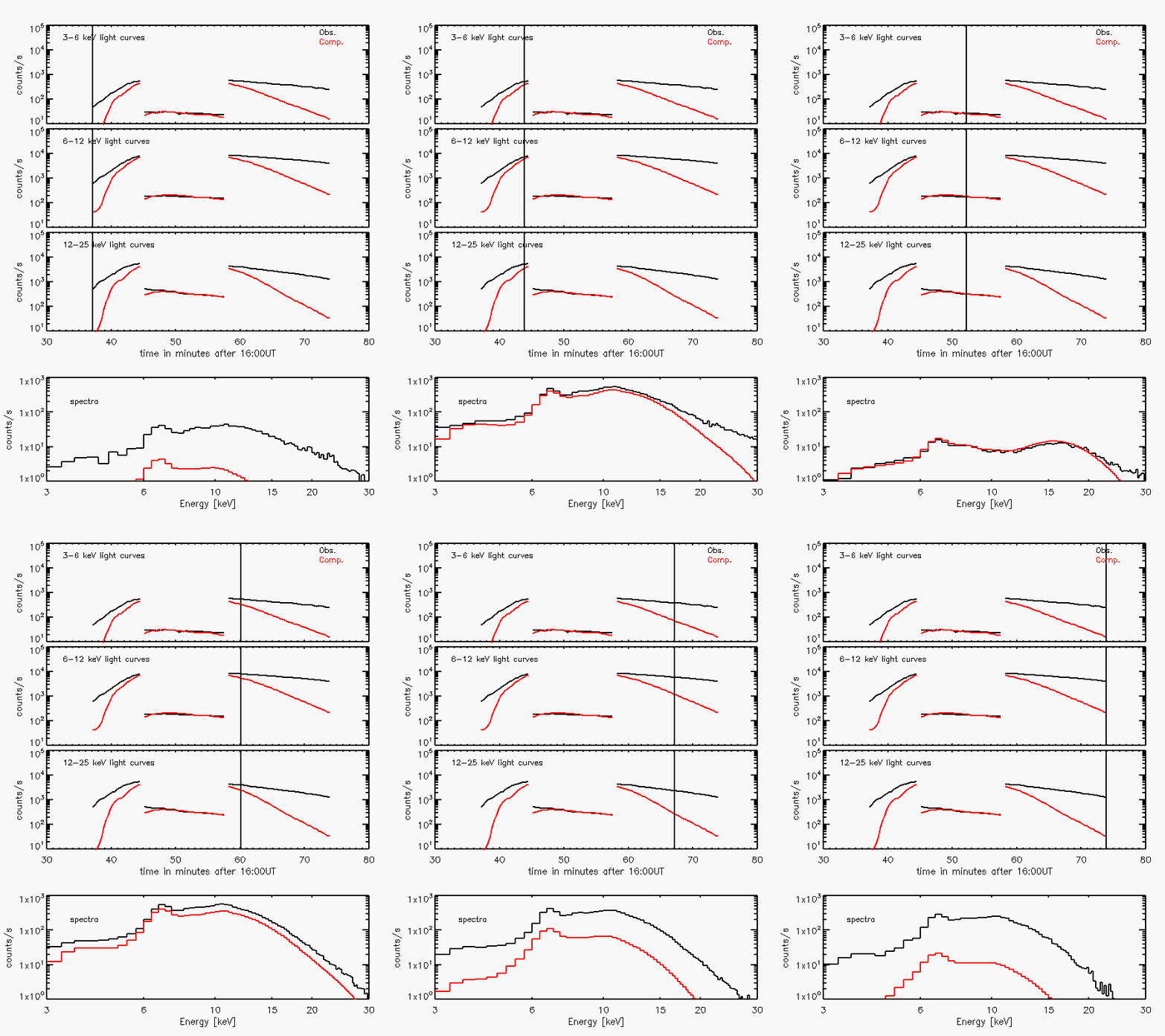
In these plots, we only compare the spectrum up to 20 keV, beyond which the spectrum is likely dominated by thick-target bremsstrahlung produced by non-thermal electrons colliding at the lower atmosphere. For most of the impulsive phase, from 16:44 UT to 16:59 UT, the synthetic spectra agree with the observations (see panels b, c, and d in Figure 10), with mean value between 0.7 and 1.3 and close to zero. From 16:50 to 16:55 UT, around the maxima of the GOES SXR light curves, the modeled thermal emission dominates up to 20 keV (see panels c and d), indicating strong heating in flare loops although the non-thermal HXR emission has become insignificant. These plots showing good agreement between the model and observations suggest that the model has rather accurately reproduced the DEM responsible for the thermal bremsstrahlung X-ray radiation in the observed range during this period.
From the start of the flare until 16:42 UT, the synthetic spectrum is lower than observed by nearly the same fraction across the energy range up to 15 keV (panel a in Figure 10). The synthetic flux at 15 keV is still smaller than observed, which may indicate a lack of high-temperature plasma in the model, but may also be due to predominant non-thermal bremsstrahlung radiation down to 15 keV. RHESSI images in the 15–20 keV energy range during this period (not shown) show that the X-ray source is rather extended, likely including emissions from both the foot-point and loop-top, which cannot be resolved with good photometric accuracy. Therefore, both scenarios are plausible. In the late phase of the flare after 17:00 UT, the modeled flux drops below the observed flux again. In this phase, thick-target HXR emission has ended, so the low flux above 15 keV is likely caused by a lack of high temperature plasma in the model. We also note that in the early and late phases of the flare, when the average ratio is far below 1, the slope becomes negative. These indicate that the model does not generate enough high temperature plasma during these periods, maybe due to a lack of heating events identified in our method. The bottom panel of the figure shows the number of heating events identified during the flare. It is seen that the number of heating events drops rather significantly both before 16:39 UT and after 16:55 UT. It appears that the shortage of heating events leads to insufficient X-ray flux in the calculation about 3 to 5 minutes later, which is roughly the timescale for temperature and density increases in newly formed flux tubes. The lack of heating events identified from lower atmospheric signatures (brightened UV or HXR foot-points) could be explained by the fact that there is neither strong conduction flux nor significant non-thermal beam to deposit enough energy at the lower atmosphere to generate observable signatures. In the rise phase, it is plausible despite the significant non-thermal HXR emission, if the non-thermal electrons are partially or largely trapped in the corona and do not reach the chromosphere to generate HXR foot points; the trapped electrons would then be a source of in situ heating in the corona. Such a mechanism has been proposed for the “pre-impulsive” phase of a few large flares [60, 11, 13, e.g.,] where non-thermal emission is observed in the corona with no identifiable HXR foot points, and may also contribute here.
Comparison between the observed and synthetic spectra, as characterized by and , provides us with observational constraints to the heating function parameters and , in addition to the observed UV and HXR signatures at the flare foot-points that constrain the time profiles of the heating rate.
IV.3 UV Emission in the Decay Phase
The long decay of TRACE 1600 Å emission in individual flaring pixels is reported by Qiu et al. [80] and Cheng et al. [18]. Flare emission in this broadband channel includes both the enhanced UV continuum and the C iv line emission. The C iv resonance doublet at 1548 Å and 1551 Å could only be emitted over a very narrow temperature range around 105 K, and therefore the C iv intensities rise when the transition region is heated with more plasma raised to 105 K during the flare. The C iv irradiance was observed to be enhanced by three to four orders of magnitude over the pre-flare emission during the impulsive phase of a large flare [5]. During the decay phase, the C iv emission is dominated by the evolution of coronal pressure [31, 41, 38]. The solar UV continuum radiation in the 1000–2000 Å wavelength range is also enhanced during the flare [19, 16, 17, e.g., ]. In particular, the continuum emission below 1682 Å is primarily contributed by bound-free transitions of Si i, which is primarily excited by the C iv doublet [65, 66]. Therefore, the continuum intensity at 1682 Å is approximately proportional to the C iv line intensity [77]. Though there is no direct C iv measurement for the M8.0 flare studied in this paper, observations of stellar flares show that the time profile of C iv is similar to the UV 1600 Å emission in solar flares observed by TRACE, both exhibiting a fast rise and a long decay [95].
In this study, we have used the rapid rise of UV emission to constrain the time, duration, and magnitude of the heating rate in individual flare loops. The gradual decay of UV emission from the same foot-points reflect the evolution of the over-lying corona that has been heated impulsively and then cools down on a much longer timescale. Using the coronal plasma properties from the model, we further calculate the C iv line emission during the decay phase to compare with the TRACE UV observation.
To calculate the C iv line emission on the solar surface, it is important to know the opacity. Doschek et al. [25] and Dere & Mason [23] measured the intensity ratio of two C iv lines at 1548 and 1550 observed on the disk, and found the ratio very close to 2:1, which is expected for optically thin lines. Doschek [24] also estimated the opacity of C iv to be 0.099 in the active-region spectrum. We therefore consider that the C iv line is optically thin. The C iv photon flux at the surface is then calculated through
| (6) |
where is the abundance of Carbon relative to Hydrogen. In this paper the solar coronal abundances of Feldman et al. [30] are used; if photospheric abundances [37, i.e.,] are used, the C iv line emission will be reduced by 15%. is the contribution function for the C iv line and is obtained from CHIANTI [22, 55] with the ionization equilibrium of Mazzotta et al. [69]. It does not change significantly when the electron density varies from cm-3 to cm-3. DEM is the transition region DEM, where measures distance along the flux tube from the base of the transition region. For each flux tube, we assume that the transition region is nearly in static equilibrium in the decay phase when the heating has finished, which is roughly when the coronal density peaks. In this case, thermal conduction is balanced by radiation, and pressure is uniform from the corona through the transition region when gravity is ignored, and the transition region DEM can be calculated as [31, 41]:
| (7) |
where , is the temperature at the base of the transition region, taken to be a nominal 104 K, and is the optically-thin radiative loss function.
The C iv line emission of one flux tube in its decay phase is calculated with equations (6) and (7) and convolved with the TRACE 1600 Å band response function to get synthetic UV flux in units of DN s-1. The left panel of Figure 12 shows an example of the computed C iv line emission in one flux tube. The computed C iv flux appears to evolve along with the observed decay, though the synthetic flux is smaller than the observed by a factor of 2. The right panel of the figure shows the sum of the synthetic UV flux in all flaring pixels in comparison with the observed total UV emission in the decay phase. The observed UV decay in a pixel is obtained by subtracting from the UV light curve the full Gaussian derived by fitting the UV rise so that the transition region response to the heating is excluded. Similar to the single-pixel comparison, the computed total C iv emission decays on the same timescale as observed, and the computed flux is lower than observed by a factor of 2 to 3.
We find this comparison satisfactory for the following reasons. First, the transition region is not exactly in static equilibrium. During the decay phase, the transition region loss usually exceeds the conductive flux, which leads to downflows from the corona, and therefore the coronal density gradually decreases. The downflow is literally an energy input into the transition region and gives rise to a greater transition region DEM than in the case of static equilibrium. Second, the UV continuum in the decay phase may be also enhanced due to irradiation from the C iv line. The observed UV emission is the sum of both the line and continuum emissions, though the continuum intensity is considered to be proportional to the line intensity. All these reasons would explain the observed UV emission being larger than the computed C iv line emission with the static equilibrium assumption. It is, nevertheless, very encouraging to find that the computed line emission decays at the same rate as the observed UV emission. In contrast, the computed X-ray emission decays faster than observed, as shown in the previous Section. Since the UV decay is derived from the same pixels whose rise phase is used to construct the loop heating rate, such comparison indirectly confirms that the rapid decay of the computed SXR flux most likely indicates the presence of additional heating events in the decay phase, which are not found in foot-point UV radiation signatures. This is consistent with decades of observations which have shown that coronal plasma temperatures decrease more slowly than would be expected from simple calculations of radiative and conductive cooling [71, 93, 94, e.g.,], implying that additional heating must be taking place despite an apparent lack of accelerated particles. These additional heating events may thus result from continuous reconnection in the corona that provides direct heating without significantly accelerating non-thermal particles, or which accelerates particles sufficiently weakly such that they thermalize in the ambient plasma at the loop-top; both scenarios lead to increased SXR coronal emission without associated chromospheric emission that could be identified in TRACE broadband UV or RHESSI HXR observations. A similar mechanism has been proposed for the so-called “EUV late phase” emission from eruptive (and often CME-associated) flares [102], where reconnection high in the corona heats post-flare loops, resulting in increased EUV coronal emission without associated foot-point brightenings.
V Discussion and Conclusions
We have analyzed and modeled an M8.0 flare on 2005 May 13 observed by TRACE, RHESSI, and GOES, in order to determine heating rates in a few thousand flare loops formed by reconnection and subsequently heated. The rapid rise of spatially resolved UV emission from the lower atmosphere is considered to be the instantaneous response to heating in the flare loops rooted at the foot points, and therefore is used to construct heating rates in individual flare loops to describe when, for how long, and by how much flare loops are heated [81]. With these heating rates, we compute the coronal plasma evolution in these loops using the 0D EBTEL model, and compare, for the first time, the computed time-dependent coronal radiation with observations by RHESSI and GOES, and as well the computed UV line emission with TRACE observations during the decay phase of flare loops. The comparison constrains parameters of the loop heating rates, which define the amount of total energy flux and the fraction of energy flux carried by chromospheric upflows driven by non-thermal beams.
The M8.0 flare studied in this paper is observed to have significant thick-target HXR emission, suggesting that the lower atmosphere is also heated by electron beams during the impulsive phase. In this process, chromospheric evaporation is driven carrying mass and energy flux back to the corona. In this study, we experimentally scale the beam-driven energy flux with the observed HXR light curve, and examine how varying the fraction of beam heating changes the modeled coronal temperature and density evolution. In general, for a given total amount of heating flux, a larger fraction of energy carried by beam driven upflow leads to higher density, lower temperature, and more rapid evolution of the coronal plasma. These properties affect the computed SXR spectrum and its time evolution, and can be compared against the spectrum observed by RHESSI. Our experiment yields an optimal set of parameters, with which, the model computed SXR light curves and spectra agree very well with observations during the rise phase and peak of the flare for more than 10 minutes.
Apart from comparison with the SXR observations, we also compute the C iv line emission at the foot of the flare loop during the decay, whose rise phase is used to construct the heating rate in the same loop. Emission in this optically-thin line during the decay phase is governed by plasma evolution in the overlying coronal loop and contributes significantly to the UV emission observed in the TRACE 1600 Å bandpass. It is shown that the computed C iv flux is about one third of the observed UV flux, which also includes the continuum radiation, and decays on the same timescale as observed. This experiment shows an avenue to model heating and cooling of spatially resolved flare loops with self-consistent constraints by high-resolution UV observations from the input (UV rise) to the output (UV decay) in the same flare loop.
These results suggest that our method, which employs all available observations to constrain flare loop heating model, is able to capture the distribution of impulsive heating rates in numerous flare loops formed and heated sequentially by magnetic reconnection. The optimal heating function parameters determined for this flare yield the peak heating flux in the range of 108–1010 ergs cm-2 s-1 for over 5000 flare loops of cross-sectional area 1″ by 1″. Notably, only 40% of this energy is carried by beam-driven upflows during the impulsive phase, with the remaining 60% contributed by in situ heating in the corona. The beam heating occurs mostly during the first ten minutes, when the flare exhibits significant thick-target HXR emission; meanwhile, the in situ heating energy in the impulsive phase amounts to 6.21030 ergs, over 3 times greater than the beam-driven contribution. In the post-impulsive phase (after 16:50 UT), the continuously expanding UV ribbons and the observed Neupert effect between the SXR derivative and UV (rather than HXR) light curves indicate that new flare loops are formed by continuous reconnection, and in situ heating in the corona is predominant, amounting to 4.11030 ergs out of the total, with negligible beam heating. The total energy used in coronal heating in this flare amounts to 1.221031 ergs, of which the total energy carried by beam-driven upflows is estimated to be only 1.91030 ergs (16%). Therefore, it appears that in situ coronal heating and thermal conduction play an important role in the energetics of this M8.0 flare, in contrast to commonly accepted models that consider the coronal thermal plasma to be largely a by-product of beam-driven heating of the lower atmosphere (chromosphere and transition region) [63, 13, 64, see also discussions by]. A survey of 37 M- and X-class flares [12] suggests that in situ heating may be significant even down to mid-C class, and therefore this heating mechanism must be considered in future studies of flare energetics.
We note that these energies set lower limits for this M8.0 flare. First, despite the excellent agreement between the model and observation in the rise phase of the flare, the model computed X-ray flux decays more quickly than observed by both GOES and RHESSI. It is most likely that magnetic reconnection and energy release continue in the high corona during the decay of the flare. These heating events might not produce significant UV foot-point emission, and are therefore not identified in our method. For comparison, Kazachenko et al. [51], Kazachenko et al. [50] analyzed the same flare, and estimated the total energy from GOES (including energy loss from radiation, conductive cooling and enthalpy flux) to be 3.11031 ergs. Second, in our experiment, we do not model heating and dynamics of the lower atmosphere, but use a simple scaling relationship to estimate the energy flux carried by non-thermal beam-driven upflows back to the corona. This amount of energy is a fraction of the total energy carried by non-thermal beams; the remainder is lost in the lower atmosphere. As a reference, we fit the HXR spectrum to a power-law distribution with the standard RHESSI software package (not shown in the paper), and, with the low-energy cutoff and spectral index from the fit, estimate the total non-thermal energy to be 7.6 ergs, about 4 times the energy carried in the upflow but, interestingly, still somewhat smaller than the energy required to heat the coronal plasma – though we note that the non-thermal energy estimate is only a loose lower bound since it depends critically on the fit low-energy cutoff, which is unbounded from below due to obscuration by the highly-dominant thermal emission.
Our experiment provides a novel method for investigating energy release in solar flares, which is governed by reconnection and substantiated in formation and heating of numerous flare loops. This approach has a few advantages. First, by analyzing the foot-point UV signatures combined with HXR observations, for the first time, we are able to identify and characterize the energy release process in a few thousand flare loops down to 1″ by 1″ scale, which is thought to be close to the basic scale of flux tubes formed in patchy reconnection. Using the same UV data, we also measure the rate of magnetic reconnection and hence are able to establish the relationship between reconnection and energy release in temporally and spatially resolved manner. Second, using the 0D EBTEL model, we are able to efficiently compute plasma properties of this large number of flux tubes, and naturally generate a time-dependent differential emission measure (DEM) from these flare loops formed and heated at different times and evolving independent of one another. Subsequently, we can predict X-ray and UV radiation signatures directly comparable with observations, which provides further constraints to our determination of energy release rates.
The method utilizes emission signatures at all available wavelengths in both the foot-points and overlying coronal loops. The dynamics of the lower atmosphere and corona are strongly coupled; they are governed by different yet coherent physics, and hence should be studied coherently. In this study, based on the insight from previous theoretical and numerical research, we employ some empirical laws to prescribe the relation between heating rates and radiation signatures. The optimal parameters obtained from the analysis can provide a reference for further investigation based on physical models, such as models of lower atmosphere heating and dynamics. We also recognize that the 0D EBTEL model has limitations in accurately describing coronal plasma properties along the loop. Nevertheless, the model is highly efficient in dealing with a few thousand flare loops and yields the first-order heating rates as useful inputs for more sophisticated loop heating models such as those by Mariska [67], Antiochos et al. [3], or Winter et al. [101]. Our study of this event shows very good agreement between observed and modeled high temperature plasma radiations (e.g., by RHESSI and GOES), but lacks observations of and therefore comparison with low temperature plasma signatures, which are crucial in understanding the flare loop evolution beyond the conduction-dominant regime. The recently launched SDO has observed many flares with AIA, the high-resolution imaging telescope, in a number of UV and EUV bands [56], and as well with the broad-band, high resolution spectrometers on the Extreme Ultraviolet Variability Experiment [103, EVE;]. These new observations, which cover coronal temperatures from 1 MK up to 20 MK, can be combined with RHESSI observations that provide information of hot (10–50 MK) plasmas, as well as information about the non-thermal emission, to fully observationally characterize the temperature distribution and its evolution (Caspi et al. 2013b, in prep.), which can be compared with – and used to constrain – our modeling. These new facilities will allow us to analyze and model flare plasmas following the entire process of heating and cooling, and also to study resolved individual flare loops in multiple wavelengths in more details, which will improve determination of the energy release rate during magnetic reconnection.
Finally, the poor comparison between model and observations during the decay phase of the flare reflects some limitations of the present method. These can be addressed by more sophisticated one-dimensional modeling that also includes the lower atmosphere, to help determine the amount of lower atmosphere radiation, such as the UV 1600 Å emission used in this study, as dependent on the heating mechanism and the amount of heating. Such effort will help clarify whether the shortage of computed flux is produced by the method missing weak heating events, or by other significant effects related to imperfect model assumptions.
References
- [1] Abbett, W. P., & Hawley, S. L. 1999, ApJ, 521, 906
- [2] Allred, J. C., Hawley, S. L., Abbett, W. P., & Carlsson, M. 2005, ApJ, 630, 573
- [3] Antiochos, S. K., MacNeice, P. J., Spicer, D. S., & Klimchuk, J. A. 1999, ApJ, 512, 985
- [4] Aschwanden, M. J., & Alexander, D. 2001, Sol. Phys., 204, 91
- [5] Brekke, P., Rottman, G. J., Fontenla, J., & Judge, P. G. 1996, ApJ, 468, 418
- [6] Brown, J. C. 1973, Sol. Phys., 31, 143
- [7] Canfield, R. C., & Gayley, K. G. 1987, ApJ, 322, 999
- [8] Cargill, P. J., Bradshaw, S. J., & Klimchuk, J. A. 2012a, ApJ, 752, 161
- [9] —. 2012b, ApJ, 758, 5
- [10] Carmichael, H. 1964, NASA Special Publication, 50, 451
- [11] Caspi, A. 2010, PhD thesis, Department of Physics, University of California, Berkeley, CA 94720-7450, USA
- [12] Caspi, A., Krucker, S., & Lin, R. P. 2013, ApJ, submitted
- [13] Caspi, A., & Lin, R. P. 2010, ApJ, 725, L161
- [14] Cheng, C.-C., Oran, E. S., Doschek, G. A., Boris, J. P., & Mariska, J. T. 1983, ApJ, 265, 1090
- [15] Cheng, C.-C., Tandberg-Hanssen, E., Bruner, E. C., et al. 1981, ApJ, 248, L39
- [16] Cheng, C.-C., Tandberg-Hanssen, E., & Orwig, L. E. 1984, ApJ, 278, 853
- [17] Cheng, C.-C., Vanderveen, K., Orwig, L. E., & Tandberg-Hanssen, E. 1988, ApJ, 330, 480
- [18] Cheng, J. X., Kerr, G., & Qiu, J. 2012, ApJ, 744, 48
- [19] Cook, J. W., & Brueckner, G. E. 1979, ApJ, 227, 645
- [20] Coyner, A. J., & Alexander, D. 2009, ApJ, 705, 554
- [21] Dennis, B. R., & Zarro, D. M. 1993, Sol. Phys., 146, 177
- [22] Dere, K. P., Landi, E., Mason, H. E., Monsignori Fossi, B. C., & Young, P. R. 1997, åps, 125, 149
- [23] Dere, K. P., & Mason, H. E. 1993, Sol. Phys., 144, 217
- [24] Doschek, G. A. 1997, ApJ, 476, 903
- [25] Doschek, G. A., Dere, K. P., & Lund, P. A. 1991, ApJ, 381, 583
- [26] Emslie, A. G. 1978, ApJ, 224, 241
- [27] —. 1980, ApJ, 235, 1055
- [28] Emslie, A. G., Li, P., & Mariska, J. T. 1992, ApJ, 399, 714
- [29] Emslie, A. G., & Nagai, F. 1985, ApJ, 288, 779
- [30] Feldman, U., Mandelbaum, P., Seely, J. F., Doschek, G. A., & Gursky, H. 1992, ApJS, 81, 387
- [31] Fisher, G. H. 1987, ApJ, 317, 502
- [32] Fisher, G. H., Canfield, R. C., & McClymont, A. N. 1984, ApJ, 281, L79
- [33] —. 1985a, ApJ, 289, 425
- [34] —. 1985b, ApJ, 289, 414
- [35] Fletcher, L., Pollock, J. A., & Potts, H. E. 2004, Sol. Phys., 222, 279
- [36] Fletcher, L., Dennis, B. R., Hudson, H. S., et al. 2011, Space Sci. Rev., 159, 19
- [37] Grevesse, N., & Sauval, A. J. 1998, ßr, 85, 161
- [38] Griffiths, N. W., Fisher, G. H., & Siegmund, O. H. W. 1998, in Astronomical Society of the Pacific Conference Series, Vol. 154, Cool Stars, Stellar Systems, and the Sun, ed. R. A. Donahue & J. A. Bookbinder, 621
- [39] Handy, B. N., Acton, L. W., Kankelborg, C. C., et al. 1999, Sol. Phys., 187, 229
- [40] Hannah, I. G., Christe, S., Krucker, S., et al. 2008, ApJ, 677, 704
- [41] Hawley, S. L., & Fisher, G. H. 1992, ApJS, 78, 565
- [42] —. 1994, ApJ, 426, 387
- [43] Hill, S. M., Pizzo, V. J., Balch, C. C., et al. 2005, Sol. Phys., 226, 255
- [44] Hirayama, T. 1974, Sol. Phys., 34, 323
- [45] Holman, G. D. 2012, ApJ, 745, 52
- [46] Hori, K., Yokoyama, T., Kosugi, T., & Shibata, K. 1997, ApJ, 489, 426
- [47] —. 1998, ApJ, 500, 492
- [48] Karlický, M., & Kosugi, T. 2004, åp, 419, 1159
- [49] Kato, T. 1976, ApJS, 30, 397
- [50] Kazachenko, M. D., Canfield, R. C., Longcope, D. W., & Qiu, J. 2012, Sol. Phys., 277, 165
- [51] Kazachenko, M. D., Canfield, R. C., Longcope, D. W., et al. 2009, ApJ, 704, 1146
- [52] Klimchuk, J. A., Patsourakos, S., & Cargill, P. J. 2008, ApJ, 682, 1351
- [53] Knight, J. W., & Sturrock, P. A. 1977, ApJ, 218, 306
- [54] Kopp, R. A., & Pneuman, G. W. 1976, Sol. Phys., 50, 85
- [55] Landi, E., Del Zanna, G., Young, P. R., Dere, K. P., & Mason, H. E. 2012, ApJ, 744, 99
- [56] Lemen, J. R., Title, A. M., Akin, D. J., et al. 2012, Sol. Phys., 275, 17
- [57] Lin, J. 2004, Sol. Phys., 219, 169
- [58] Lin, J., & Forbes, T. G. 2000, J. Geophys. Res., 105, 2375
- [59] Lin, R. P., Dennis, B. R., Hurford, G. J., et al. 2002, Sol. Phys., 210, 3
- [60] Lin, R. P., Krucker, S., Hurford, G. J., et al. 2003, ApJ, 595, L69
- [61] Liu, C., Lee, J., Gary, D. E., & Wang, H. 2007, ApJ, 658, L127
- [62] Longcope, D., Beveridge, C., Qiu, J., et al. 2007, Sol. Phys., 244, 45
- [63] Longcope, D. W., Des Jardins, A. C., Carranza-Fulmer, T., & Qiu, J. 2010, Sol. Phys., 267, 107
- [64] Longcope, D. W., & Guidoni, S. E. 2011, ApJ, 740, 73
- [65] Machado, M. E., & Henoux, J.-C. 1982, åp, 108, 61
- [66] Machado, M. E., & Mauas, P. J. 1986, in NASA Conference Publication, Vol. 2449, NASA Conference Publication, ed. B. R. Dennis, L. E. Orwig, & A. L. Kiplinger, 271–275
- [67] Mariska, J. T. 1987, ApJ, 319, 465
- [68] Mariska, J. T., Emslie, A. G., & Li, P. 1989, ApJ, 341, 1067
- [69] Mazzotta, P., Mazzitelli, G., Colafrancesco, S., & Vittorio, N. 1998, åps, 133, 403
- [70] Mewe, R. 1972, Sol. Phys., 22, 459
- [71] Moore, R., McKenzie, D. L., Svestka, Z., et al. 1980, in Skylab Solar Workshop II, ed. P. A. Sturrock, 341–409
- [72] Nagai, F. 1980, Sol. Phys., 68, 351
- [73] Nagai, F., & Emslie, A. G. 1984, ApJ, 279, 896
- [74] Neupert, W. M. 1968, ApJ, 153, L59
- [75] Peres, G., Serio, S., Vaiana, G. S., & Rosner, R. 1982, ApJ, 252, 791
- [76] Pesnell, W. D., Thompson, B. J., & Chamberlin, P. C. 2012, Sol. Phys., 275, 3
- [77] Phillips, K. J. H., Bromage, G. E., & Doyle, J. G. 1992, ApJ, 385, 731
- [78] Pizzo, V. J., Hill, S. M., Balch, C. C., et al. 2005, Sol. Phys., 226, 283
- [79] Qiu, J., Lee, J., Gary, D. E., & Wang, H. 2002, ApJ, 565, 1335
- [80] Qiu, J., Liu, W. J., Hill, N., & Kazachenko, M. 2010, ApJ, 725, 319
- [81] Qiu, J., Liu, W.-J., & Longcope, D. W. 2012, ApJ, 752, 124
- [82] Reeves, K. K., & Moats, S. J. 2010, ApJ, 712, 429
- [83] Reeves, K. K., & Warren, H. P. 2002, ApJ, 578, 590
- [84] Reeves, K. K., Warren, H. P., & Forbes, T. G. 2007, ApJ, 668, 1210
- [85] Reeves, K. K., Winter, H. D., & Larson, N. L. 2012, in Astronomical Society of the Pacific Conference Series, Vol. 455, 4th Hinode Science Meeting: Unsolved Problems and Recent Insights, ed. L. Bellot Rubio, F. Reale, & M. Carlsson, 199
- [86] Smith, D. M., Lin, R. P., Turin, P., et al. 2002, Sol. Phys., 210, 33
- [87] Somov, B. V., & Kosugi, T. 1997, ApJ, 485, 859
- [88] Somov, B. V., Sermulina, B. J., & Spektor, A. R. 1982, Sol. Phys., 81, 281
- [89] Somov, B. V., Spektor, A. R., & Syrovatskii, S. I. 1981, Sol. Phys., 73, 145
- [90] Spitzer, L. 1962, Physics of Fully Ionized Gases, ed. Spitzer, L.
- [91] Sterling, A. C., Shibata, K., & Mariska, J. T. 1993, ApJ, 407, 778
- [92] Sturrock, P. A. 1966, Nature, 211, 695
- [93] Veronig, A., Vršnak, B., Dennis, B. R., et al. 2002a, åp, 392, 699
- [94] Veronig, A., Vršnak, B., Temmer, M., & Hanslmeier, A. 2002b, Sol. Phys., 208, 297
- [95] Vilhu, O., Muhli, P., Huovelin, J., et al. 1998, AJ, 115, 1610
- [96] Warren, H. P. 2006, ApJ, 637, 522
- [97] Warren, H. P., & Doschek, G. A. 2005, ApJ, 618, L157
- [98] Warren, H. P., & Warshall, A. D. 2001, ApJ, 560, L87
- [99] White, S. M., Thomas, R. J., & Schwartz, R. A. 2005, Sol. Phys., 227, 231
- [100] Winebarger, A. R., & Warren, H. P. 2004, ApJ, 610, L129
- [101] Winter, H. D., Martens, P., & Reeves, K. K. 2011, ApJ, 735, 103
- [102] Woods, T. N., Hock, R., Eparvier, F., et al. 2011, ApJ, 739, 59
- [103] Woods, T. N., Eparvier, F. G., Hock, R., et al. 2012, Sol. Phys., 275, 115


