LTH–974
Proton Stability,
Gauge Coupling Unification
and a Light in Heterotic–string Models
Alon E. Faraggi11 1 E-mail address: faraggi@amtp.liv.ac.uk and Viraf M. Mehta22 2 E-mail address: Viraf.Mehta@liv.ac.uk
Department of Mathematical Sciences
University of Liverpool, Liverpool, L69 7ZL, United Kingdom
We explore the phenomenological viability of a light in heterotic–string models, whose existence has been motivated by proton stability arguments. A class of quasi–realistic string models that produce such a viable are the Left–Right Symmetric (LRS) heterotic–string models in the free fermionic formulation. A key feature of these models is that the matter charges under do not admit an embedding. The light in the LRS heterotic–string models forbids baryon number violating operators, while allowing lepton number violating operators, hence suppressing proton decay yet allowing for sufficiently small neutrino masses via a seesaw mechanism. We show that the constraints imposed by the gauge coupling data and heterotic–string coupling unification nullify the viability of a light in these models. We further argue that agreement with the gauge coupling data necessitates that the charges admit an embedding. We discuss how viable string models with this property may be constructed.
1 Introduction
The discovery of the Higgs boson at the LHC lends further credence to the hypothesis that the Standard Model (SM) provides a viable effective parametrisation of all subatomic interactions up to the GUT or heterotic–string unification scales. Support for this possibility stems from: the matter gauge charges; proton longevity; suppression of neutrino masses; and the logarithmic evolution of the SM parameters in its gauge and matter sectors. Preservation of the logarithmic running in the SM scalar sector entails that it must be augmented by a new symmetry. A concrete framework that fulfils the task is given by supersymmetry.
The supersymmetric extension of the SM introduces dimension four and five baryon and lepton number violating operators that mediate proton decay. This problem is particularly acute in the context of heterotic–string derived constructions, in which one cannot assume the existence of global or local discrete symmetries that simply forbid the undesired operators. Indeed, the issue has been examined in the past by a number of authors [1]. The avenues explored range from the existence of matter parity at special points in the moduli space of specific models, to the emergence of non–abelian custodial symmetries in some compactifications. However, a caveat to these arguments is that in addition to suppressing the proton decay mediating operators, one must also ensure that the mass terms of left–handed neutrinos are sufficiently suppressed. That is, while baryon number should be conserved to ensure proton longevity, lepton number must be broken to allow for suppression of left–handed neutrino masses. In heterotic–string constructions, due to the absence of higher–order representations of the Grand Unified Theory [2], one typically has to break lepton number by one unit, which generically results in both lepton and baryon number violation. An alternative solution to this conundrum is obtained if an additional gauge symmetry, beyond the SM gauge group, remains unbroken down to low scales. An additional abelian gauge symmetry, which is broken near the TeV scale, may also explain the suppression of the –term in the supersymmetric potential [3].
The possibility of a low scale arising from heterotic–string inspired models has a long history and continues to attract wide interest [4]. Surprisingly, however, keeping a in explicit string derived constructions, unbroken down to the low scale, turns out to be notoriously difficult, as such an extra symmetry must satisfy a variety of phenomenological constraints. Obviously, to play a role in the suppression of proton decay mediating operators (PDMOs) implies that the SM matter states are charged under this symmetry. While forbidding baryon number violation, it should allow for lepton number violation, required for the suppression of neutrino masses. Furthermore, it should be family universal, otherwise there is a danger of generating Flavour Changing Neutral Currents (FCNC), or of generating the PDMOs via mixing. The additional symmetry should also allow for the fermion Yukawa couplings to electroweak Higgs doublets and must be anomaly free. Explicit string models that do give rise to an extra symmetry with the required properties are the left–right symmetric models of [5, 6]. The existence of the required symmetry in explicit string constructions ensures that, in these examples, the extra is free of any gauge and gravitational anomalies. In [7] we constructed toy string–inspired models that are compatible with the charge assignments in the string derived models. In these models, the proton lifeguarding extra symmetry can, in principle, remain unbroken down to low scales.
An additional constraint that must be imposed on the extra gauge and matter states that arise in the models, is compatibility with the gauge parameters, and . The perturbative heterotic–string predicts that all the gauge couplings are unified at the string unification scale, , which is of the order . Nonperturbatively, the heterotic–string can be pushed to the GUT unification scale, , of the order [8]. In this paper we study the constraints that are imposed on the string inspired models by gauge coupling unification and show that the gauge coupling data is not in agreement with the left–right symmetric heterotic–string models. The origin for the disagreement lies in the specific charges, which do not admit an embedding. For comparison we also perform the analysis for charges that maintain the embedding and show that, in this case, agreement with the data is achieved. We discuss how viable string derived models that preserve the embedding may be constructed.
2 Additional s in free fermionic models
In this section we review the structure of the free fermionic models. We focus on the extra symmetries that arise in the models and the charges of the matter states. We elaborate on the gauge symmetry breaking patterns induced by the Generalised GSO (GGSO) projections but concentrate here on the group theory structure and the matter charges. Further details of the free fermionic models and their construction are found in earlier literature [5, 9, 10, 11, 12, 13, 14, 15, 16]. The free fermionic models correspond to orbifold compactifications at special points in the moduli space [17]. It should be emphasized that our results are applicable to the wider range of orbifold models because they merely depend on the symmetry breaking patterns of the observable gauge symmetry.
Free fermionic heterotic–string models are constructed by specifying a consistent set of boundary condition basis vectors and the associated one–loop GGSO phases [9]. These basis vectors span a finite additive group, , where the physical states of a given sector, , are obtained by acting on the vacuum with bosonic and fermionic operators and by applying the GGSO projections. The charges, with respect to the unbroken Cartan generators of the four dimensional gauge group, are given by:
| (2.1) |
where is the boundary condition of the complex world–sheet fermion in the sector , and is a fermion number operator counting each mode of once ( minus once). For periodic fermions with , the vacuum is a spinor representing the Clifford algebra of the zero modes. For each periodic complex fermion, , there are two degenerate vacua, , annihilated by the zero modes, and , with fermion numbers respectively.
Three generation models in the free fermionic construction have been obtained by using two constructions: the first were the NAHE based models [13]; and the second class of models are those constructed by the classification method of [15]. The important distinction between the two cases is that the latter has only been applied for symmetric orbifolds, whereas, in the former, most of the constructions utilise asymmetric boundary conditions.
In NAHE based models [5, 10, 11, 12, 14] the first set of five basis vectors, , are fixed; , and correspond to the three twisted sectors of the orbifold and is the spacetime supersymmetry generator. The gauge symmetry at the level of the NAHE set is with spacetime supersymmetry. The second stage of the construction consists of adding three additional basis vectors to the NAHE set. The additional vectors reduce the number of generations to three and simultaneously break the four dimensional group. The symmetry is broken to one of its maximal subgroups: (FSU5) [10]; (SLM) [11]; (PS) [12]; (LRS) [5]; and (SU421) [14].
An important distinction between the last two cases and the first three is in regard to the anomalous symmetry that arises in these models [5, 14, 18]. The Cartan subalgebra of the observable rank eight gauge group is generated by eight complex fermions, denoted by , where are the Cartan generators of the group and generate three symmetries, denoted by . In the FSU5, PS and SLM cases the , as well as their linear combination,
| (2.2) |
are anomalous, whereas in the LRS and SU421 models they are anomaly free. The distinction can be seen to arise from the symmetry breaking patterns induced in the two cases from the underlying toroidal model in four dimensions. Starting from the , in the first case the symmetry is broken to by the choice of GGSO projection phases in the fermionic models, or equivalently by a Wilson line in the corresponding orbifold models. The basis vectors and break the symmetry further to . Alternatively, we can implement the and twists in the vacuum, which break the gauge symmetry to . The Wilson line breaking then reduces the symmetry to . It is then clear that the becomes anomalous because of the symmetry breaking to and the projection of some states from the spectrum by the GGSO projections [18]. On the other hand, the LRS and SU421 heterotic–vacua arise from an vacuum with gauge symmetry [5, 14]. In this case, one of the factors produces the observable gauge symmetry and the second is hidden. The important point here is that these models circumvent the embedding. Hence, in these cases, the does not have an embedding and therefore remains anomaly free.
The case of the symmetric orbifolds studied in [15] only allows for models with an embedding of . Thus, in these models is, generically, anomalous. There is, however, a class of models in which it is anomaly free. This is the case in the self–dual models under the spinor–vector duality of [19]. In these models the number of spinorial representations and the number of vectorial representations, arising from the twisted sectors is identical, although the symmetry is broken. This situation occurs when the spinorial and vectorial representations are obtained from different fixed points of the toroidal orbifold. A self–dual, three generation model with unbroken symmetry is given in ref. [15], however, a viable model, of this type, with broken symmetry has not been constructed to date.
Alternatively, we may construct as an anomaly free combination by following a different symmetry breaking pattern to the discussed above. Originally, the breaking is achieved by projecting the vector bosons that arise in the spinorial representation of and enhance the symmetry to . We may construct models in which these vector bosons are not projected and, thus, the symmetry is broken to a different subgroup. Examples of such models include the three generation models of [20]. In this case, the is anomaly free by virtue of its embedding in the enhanced symmetry.
3 Gauge coupling analysis
In this section we present a comparative analysis of the two classes mentioned above. It will be instructive to specify a model in each class:
- •
Model I: This model was first presented in [7]. In this case the extra does not admit an embedding, i.e. .
- •
Model II: This model preserves the embedding of the and is akin to models arising in string inspired models [4].
Before proceeding with the gauge coupling analysis, it is instructive to detail the symmetry breaking patterns applicable to both models. The SM gauge group will be embedded, for our analysis, in . As previously mentioned, this is broken to the LRS gauge group via the addition of basis vectors, at the string scale, . The is then broken at some intermediate scale, . An anomaly free combination that remains is the which is required to survive to low energies to preserve proton longevity [6, 7].
In our analysis we vary the unification scale in the range . The lower scale is the natural MSSM unification scale [21], , whereas the higher scale corresponds to the heterotic–string unification scale [22], . This factor of 20 discrepancy was discussed in [23] and it was concluded that intermediate matter thresholds contributed enough to overcome the difference, allowing coupling unification in a wide class of realistic free–fermionic string models [24]. From the spectra of our models, we will see that it is natural to include intermediate matter thresholds to achieve string unification. It has also been demonstrated that nonperturbative effects arising in heterotic M–theory [25] can push the unification scale down to the MSSM unification scale [8]. Our aim here is to study, qualitatively, the question of gauge coupling unification in the LRS heterotic–string models. In particular, to demonstrate that a low scale in these models is incompatible with the gauge coupling data at the electroweak scale. The novel feature of the LRS models is the charge assignments. These admit an embedding and therefore similar charge assignments also arise in heterotic M–theory and so we take the unification scale to vary between and to allow for the possible nonperturbative effects. We contrast the analysis in the LRS heterotic–string models with the models that admit the embedding of the charges. In both models there are four intermediate scales between and , corresponding to:
- :
breaking scale. The neutral components of acquire a VEV to break the symmetry and leave the unbroken.
- :
Colour triplet scale. The additional colour triplets in our model acquire a mass at this scale. This will also resolve the discrepancy between the MSSM unification scale and string scale unification.
- :
breaking scale. The is broken at this scale by singlets acquiring VEVs. The anomaly cancelling doublets also acquire mass at this scale and only the MSSM spectrum survives to lower scales.
- :
Supersymmetry breaking scale. The current bounds from the LHC will be included here to get a phenomenologically viable supersymmetry scale. Only the SM states remain down to the –scale, at which the gauge data is extracted. Threshold corrections for the top quark and Higgs boson are included in the analysis.
In addition, due to the extra abelian gauge symmetry acting as our proton protector, should be sufficiently low in order for adequate suppression of induced PDMOs [6, 7] . By starting from the string scale and evolving the couplings down to , our analysis may test whether the predictions of these models are in accordance with low–energy experimental data.
Low–energy inputs
Renormalization Group Equations
For the analyses of both models, we follow [23]. String unification implies that the SM gauge couplings are unified at the heterotic–string scale. The one–loop renormalization group equations (RGEs) for the couplings are given by
| (3.2) |
where are the one–loop beta–function coefficients, and represents possible corrections from the additional gauge or matter states. By solving the one–loop RGEs we obtain expressions for and . In each model, we initially assume the MSSM spectrum between the string scale, , and the scale, , and treat all perturbations as effective correction terms. At the string unification scale we have
| (3.3) |
where is the canonical normalisation. Thus, the expression for takes the general form [23]
| (3.4) |
with taking similar form with corresponding corrections. Here represents the one–loop contributions from the spectrum of the MSSM between the unification scale and the scale. The following three terms correspond to corrections from the intermediate matter thresholds, the light SUSY thresholds, and the intermediate vector bosons corresponding to the symmetry breaking. The last term,
| (3.5) |
includes the corrections due to heavy string thresholds, and those arising from Yukawa couplings, two–loops and scheme conversion. These corrections are small and are neglected for this demonstrative analysis.
For we obtain
| (3.6) | ||||
where and are the intermediate gauge and matter scales discussed earlier. Similarly for , we have:
| (3.7) | ||||
A subtle issue in the analysis of gauge coupling unification in string models is the normalisation of the generators. In GUTs the normalisation of abelian generators is fixed by their embedding in non–abelian groups. However, in string theory the non–abelian symmetry is not manifest, and the proper normalisation of the currents is obscured. The normalisation in string models that utilise a world–sheet conformal field theory construction is fixed by their contribution to the conformal dimensions of physical states. The procedure for fixing the normalisation was outlined in [23, 28] and we repeat it here for completeness.
In the free fermionic heterotic–string models, the Kač–Moody level of non–abelian group factors is always one. In general, a given current, , in the Cartan subalgebra of the four dimensional gauge group, is a combination of the simple world–sheet currents , corresponding to individual world–sheet fermions, . then takes the form , where the are model dependent coefficients. Each is normalised to one, so that , and each of the linear combinations must also be normalised to one. The proper normalisation coefficient for the linear combination is given by , and the properly normalised current is, thus, given by .
In general, the Kač–Moody level, , of a generator can be deduced from the operator product expansion between two of the currents, and is given by
| (3.8) |
The result is generalised to when the is a combination of several s with different normalisations. This procedure is used to determine the Kač–Moody level, , of the weak–hypercharge generator, as well as that of any other combination in the effective low–energy field theory.
In the LRS heterotic–string models, the symmetry is broken to , where the combinations of world–sheet currents
| (3.9) |
and
| (3.10) |
generate and , respectively, where the latter is the diagonal generator of . The weak–hypercharge is then given by
| (3.11) | ||||
The symmetry of is incorporated in the analysis at the scale, where above this scale the multiplets are in representations of the LRS gauge group and below the scale they are in SM representations. The weak-hypercharge coupling relation is given by
3.1 Coupling unification in LRS heterotic–string models
This model is an example of a three generation, free fermionic model that yields an unbroken, anomaly free symmetry. Heterotic–string models with this property break the symmetry to the left–right symmetric subgroup [5] and are therefore supersymmetric and completely free of gauge and gravitational anomalies. The symmetry in the string models is an anomaly free, family universal symmetry that forbids the dimension four, five and six PDMOs, while allowing for the SM fermion mass terms. A combination of , and remains unbroken down to low energies and forbids baryon number violation while allowing for lepton number violation. Hence, it allows for the generation of small left–handed neutrino masses via a seesaw mechanism, specifically an extended seesaw with the singlets, [5, 7]. Proton decay mediating operators are only generated when the is broken. Thus, the scale of the breaking is constrained by proton lifetime limits and can be within reach of the contemporary experiments. A field theory model demonstrating these properties was presented in [7].
Spectrum
| Field | ||||||||
|---|---|---|---|---|---|---|---|---|
The spectrum of our model above the left–right symmetry breaking scale is summarised in Table 1. The spectrum below the intermediate symmetry breaking scale is shown in Table 2. The spectra above and below the breaking scale are both free of all gauge and gravitational anomalies. Hence, the combination given in equation (3.14) is viable to low energies.
| Field | ||||||||
|---|---|---|---|---|---|---|---|---|
The heavy Higgs’, that break the , along a flat direction, leave the orthogonal combination
| (3.14) |
unbroken. Here, the index allows for the possibility that the heavy Higgs sector contains more than two fields, as is typically the case in the string constructions. Further discussion of this model, including a trilinear level superpotential, can be found in [7]. Here we notice that the incomplete representations added to the MSSM may cause problems with gauge coupling unification. The induced gauge anomalies in the diagrams require the addition of , , , which differ from the case. The addition of triplets may help subdue any adverse effects and will also give scope for the inclusion of intermediate matter scales.
Renormalization group analysis
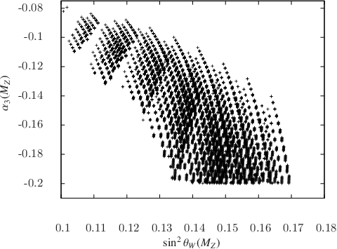
The properly normalised –function coefficients are shown in Tables 1 and 2. The numerical output of equation (3.6) and (3.7) is generated subject to the variation of the scales and is displayed in Figure 1. The intermediate scales are varied to find phenomenologically viable areas of the parameter space. The scales and ranges of and were first restricted to the experimentally allowed regions and then also allowed to take values outside this range. The hierarchy of scales was constrained to be
| (3.15) |
To this end, we restricted the allowed range of and to five sigma deviations from the central values shown in eq (3.1). The RGEs were run in Mathematica. Restricting the output to the experimentally constrained interval produced no phenomenologically viable results. Allowing the values of and to run freely and restricting the relevant mass scales to (in GeV)
| (3.16) | |||||||
also produced no phenomenologically viable results, as shown in Figure 1.
Contrasting analysis with embedding of
To further elucidate the constraints on the LRS heterotic–string models arising from coupling unification, we contrast the outcome with the corresponding results when the charges are embedded in representations. For models that allow the embedding of the charges, the spectrum consists of three generations of s that decompose under as:
| (3.17) |
Under , this results in a similar spectrum to the LRS model. The 16 decomposes exactly as for the LRS model,
| (3.18) | |||||||
with the proviso that the charges under take the same sign. The 10 decomposes as
| (3.19) | ||||||||||
The remaining singlets are neutral under the SM gauge group and are used to break the . In addition to the complete representations above, the spectrum includes a bidoublet,
| (3.20) |
that facilitates gauge coupling unification. The model also contains the pair of heavy Higgs right–handed doublets,
| (3.21) |
that break the intermediate symmetry. We run the RGEs in exactly the same way as shown for the LRS model, constraining the mass scales to the hierarchy
| (3.22) |
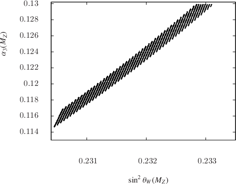
In this model we find that unification does occur, as found in previous literature. We note that the phenomenologically viable results (see Figure 2) required GeV as expected. The intermediate scales were found to be (in GeV)
| (3.23) | ||||||||||
with between TeV. In this case we have taken the mass of the vector–like doublets, , and triplets, to be degenerate, which is the case in inspired models, as they are generated by the same singlet VEV. String models afford more flexibility that we do not make use of in our analysis here. Fine–tuning the allows for to be in agreement with current experimental bounds.
The contrast between the two cases can be elucidated further by examining more closely the contributions of the intermediate gauge and matter thresholds to and . Using the general expressions in equations (3.6) and (3.7) we find that, in the case of the spectrum and charge assignments in the LRS heterotic–string model, shown in Tables 1 and 2, the threshold corrections from intermediate gauge and matter scales are given by
| (3.24) | ||||
In the case of models that admit an embedding of the charges, the same threshold corrections are given by
| (3.25) | ||||
If we take to coincide with the MSSM unification scale and with as well, then the first lines in equations (3.6) and (3.7), which only contain the MSSM contributions, are in good agreement with the observable data. The corrections arising from the intermediate gauge and matter thresholds in equations (3.24) and (3.25) then have to cancel. We see from equation (3.24) that the corrections from the intermediate doublet and triplet thresholds contribute with equal sign in . For , the corrections from these thresholds contribute with opposite sign, but the contribution of the doublets outweigh the contribution of the triplets. We may compensate for the negative contribution from the extra doublets by lowering the breaking scale. Requiring that necessitates that . Keeping the extra triplets at the GUT scale, and the scale at then yields rough agreement with but gross disagreement with . Lowering the triplet scale improves the agreement with but conflicts with the data for . We therefore conclude that a low scale in the LRS heterotic–string models is incompatible with the gauge data at the –boson scale. In contrast, from equation (3.25) we see that the corresponding corrections cancel each other, provided that . This is the case as both are generated by the breaking VEV. This cancellation is, of course, the well known cancellation that occurs when the representations fall into multiplets. Allowing to be at then compensates for the SUSY threshold at , enabling accommodations of the low–energy data, as illustrated in Figure 2.
4 String models with embedding
The low scale in the string models is, in essence, a combination of the Cartan generators, , that are generated by the right–moving complex world–sheet fermions , together with a symmetry, embedded in the GUT, and is orthogonal to the weak hypercharge. Whether, or not, the symmetry is anomaly free depends on the specific symmetry breaking pattern induced by the GGSO projections. As we discussed above, in the FSU5, PS and SLM the symmetry is anomalous, whereas in the LRS models it is anomaly free. The difference stems from the fact that in the former cases the combination for admits the embedding but in the latter it does not. On the other hand, as we have seen in Section 3, the embedding allows for compatibility with the low scale gauge coupling data. The in the LRS models, which do not admit the embedding, is constrained to be heavier than at least GeV. Gauge coupling data, therefore, seems to indicate that the embedding of the charges is necessary. We emphasize that the indication is that the charges must admit an embedding and not that the symmetry is actually realised. An illustration of this phenomenon is the existence of self–dual models under the spinor–vector duality without enhancement [19]. The question then arises as to how one constructs heterotic–string models with anomaly free , which admit an embedding. Here we discuss how viable heterotic–string models with embedding of the charges may be obtained. The main constraint being that the extra symmetry has to be anomaly free. For this purpose, we first give a general overview as to how the gauge symmetry is generated in the string models.
The vector bosons that generate the four dimensional gauge group in the string models arise from two principal sectors: the untwisted sector and the sector . In the –sector the complex right–moving world–sheet fermions, that generate the Cartan subalgebra of the observable gauge group, are all periodic. At the level of the heterotic–string in ten dimensions, the vector bosons of the observable are obtained from the untwisted sector and from the –sector. Under the decomposition , the adjoint representation decomposes as , where the adjoint representation is obtained from the untwisted sector and the spinorial representation is obtained from the –sector. The set produces a model with spacetime supersymmetry in four dimensions. The gauge symmetry arising in this model, at a generic point in the compactified space, is either or depending on the GGSO phase .
Adding the basis vectors and reduces the spacetime supersymmetry to . The observable gauge symmetry reduces from to or . Additional vectors reduce the gauge symmetry further. Aside from the model of [20], all the quasi–realistic free fermionic models follow the second symmetry breaking pattern. That is, in all these models, the vector bosons arising from the –sector are projected out.
We consider, then, the symmetry breaking pattern induced by the following boundary condition assignments in two separate basis vectors
| (4.1) | |||||
| (4.2) |
The assignment in equation (4.1) reduces the untwisted gauge symmetry to , however the assignment in eq. (4.2) reduces it to . Thus, the inclusion of equations (4.1) and (4.2) in two separate boundary condition basis vectors reduces the gauge symmetry to , where and . For appropriate choices of the GGSO projection coefficients, the vector bosons arising from the –sector enhance the arising from the untwisted sector to , where
| (4.3) | |||||
| (4.4) | |||||
| (4.5) |
and are embedded in and , respectively, and is given by equation (2.2). The matter representations charged under this group arise from the sectors and are complemented by states from to form the ordinary representations of the Pati–Salam model. The difference, as compared to the Pati–Salam string models of [12], is that is anomaly free. The reason is that all the states of the representation of are retained in the spectrum, whereas in the Pati–Salam models of [12] the corresponding states are projected out. The symmetry breaking of the Pati–Salam group is induced by the VEV of the heavy Higgs in the representation of . In addition to the weak–hypercharge, this VEV leaves the unbroken combination
| (4.6) |
which is anomaly free and admits the embedding of the charges.
5 Conclusions
In this paper we examined the gauge coupling unification constraints imposed on a low scale arising in LRS heterotic–string derived models. The existence of a low–scale in these models guarantees that PDMOs are sufficiently suppressed. However, we have shown that the hypothesis of a low scale in these models is incompatible with the gauge coupling data at the electroweak scale. We contrasted this result with the corresponding result in string models that admit an embedding of the charges. In the latter case the possibility of a low scale is viable. We further discussed how heterotic–string models that admit the embedding may be obtained in the free fermionic formulation, though an explicit three generation viable model is yet to be constructed. Similarly, a more complete analysis of the phenomenological realisation of this symmetry in heterotic–string models is warranted and will be reported in future publications. We also remark that other symmetries that have been proposed in the literature to suppress proton decay mediating operators [4, 29] have also been invalidated due to neutrino masses and other constraints [6]. The enigma of the proton lifetime in heterotic–string unification continues to serve as an important guide in the search for viable string vacua.
Acknowledgements
AEF thanks Subir Sarkar and Theoretical Physics Department at the University of Oxford for hospitality. This work was supported in part by the STFC (PP/D000416/1).
References
- [1]
R. Arnowitt and P. Nath, Phys. Rev. Lett. 62 (1989) 2225;
J. Ellis, J.L. Lopez and D.V. Nanopoulos, Phys. Lett. B252 (1990) 53;
A.E. Faraggi, Nucl. Phys. B428 (1994) 111; Phys. Lett. B339 (1994) 223; Phys. Lett. B398 (1997) 88; Phys. Lett. B398 (1997) 95;
J. Ellis, A.E. Faraggi and D.V. Nanopoulos, Phys. Lett. B419 (1998) 123;
T. Araki et al, Phys. Rev. D76 (2007) 066006;
S. Forste, H.P. Nilles, S. Ramos–Sanchez and P.K.S. Vaudrevange, Phys. Lett. B693 (2010) 386;
R. Kappl et al, Nucl. Phys. B847 (2011) 325. - [2] K.R. Dienes and J. March–Russell, Nucl. Phys. B479 (1996) 113.
- [3] G. Cleaver, M. Cvetic, J.R. Espinosa, L.L. Everett and P. Langacker, Phys. Rev. D57 (1998) 2701.
- [4]
G. Costa, J.R. Ellis, G.L. Fogli, D.V. Nanopoulos and F. Zwirner,
Nucl. Phys. B297 (1988) 244;
F. Zwirner, Int. J. Mod. Phys. AA3 (1988) 49;
J.L. Hewett, T.G. Rizzo, Phys. Rep. 183 (1989) 193;
Y. Y. Komachenko and M. Y. Khlopov, Sov. J. Nucl. Phys. 51 (1990) 692; Yad. Fiz. 51 (1990) 1081;
A.E. Faraggi and D.V. Nanopoulos, Mod. Phys. Lett. A6 (1991) 61;
A. Leike, Phys. Rep. 317 (1999) 143;
S.F. King, S. Moretti, R. Nevzorov, Phys. Rev. D73 (2006) 035009;
P. Langacker, Rev. Mod. Phys. 81 (2009) 1199;
P. Athron, S.F. King, D.J. Miller, S. Moretti and R. Nevzorov, Phys. Rev. D80 (2009) 035009;
M. Ambroso and B.A. Ovrut, Int. J. Mod. Phys. A26 (2011) 1569;
A. Belyaev, S.F. King and P. Svantesson, arXiv:1303.0770 [hep-ph]. - [5] G.B. Cleaver, A.E. Faraggi and C. Savage, Phys. Rev. D63 (2001) 066001.
- [6]
A.E. Faraggi, Phys. Lett. B499 (2001) 147;
C. Coriano, A.E. Faraggi and M. Guzzi, Eur. Phys. Jour. C53 (2008) 421. - [7] A.E. Faraggi and V.M. Mehta, Phys. Rev. D84 (2011) 086006.
- [8] E. Witten, Nucl. Phys. B460 (1996) 506.
- [9]
H. Kawai, D.C. Lewellen, and S.H.-H. Tye,
Nucl. Phys. B288 (1987) 1;
I. Antoniadis, C. Bachas, and C. Kounnas, Nucl. Phys. B289 (1987) 87;
I. Antoniadis and C. Bachas, Nucl. Phys. B289 (1987) 87. - [10] I. Antoniadis, J. Ellis, J. Hagelin and D.V. Nanopoulos Phys. Lett. B231 (1989) 65.
- [11]
A.E. Faraggi, D.V. Nanopoulos and K. Yuan,
Nucl. Phys. B335 (1990) 347;
A.E. Faraggi, Phys. Lett. B278 (1992) 131; Nucl. Phys. B387 (1992) 239;
G.B. Cleaver, A.E. Faraggi and D.V. Nanopoulos, Phys. Lett. B455 (1999) 135. - [12]
I. Antoniadis, G.K. Leontaris and J. Rizos,
Phys. Lett. B245 (1990) 161;
G.K. Leontaris and J. Rizos, Nucl. Phys. B554 (1999) 3;
K. Christodoulides, A.E. Faraggi and J. Rizos, Phys. Lett. B702 (2011) 81. - [13] A.E. Faraggi and D.V. Nanopoulos, Phys. Rev. D48 (1993) 3288.
- [14] G.B. Cleaver, A.E. Faraggi and S.E.M. Nooij, Nucl. Phys. B672 (2003) 64.
- [15]
A.E. Faraggi, C. Kounnas, S. Nooij and J. Rizos, Nucl. Phys. B695 (2004) 41;
A.E. Faraggi, C. Kounnas and J. Rizos, Phys. Lett. B648 (2007) 84. - [16] B. Assel, K. Christodoulides, A.E. Faraggi, C. Kounnas and J. Rizos, Phys. Lett. B683 (2010) 306; Nucl. Phys. B844 (2011) 365
- [17]
A.E. Faraggi, Phys. Lett. B326 (1994) 62;
Phys. Lett. B544 (2002) 207;
A.E. Faraggi, S. Forste and C. Timirgaziu, JHEP 0608, (2006) 057;
R. Donagi and A.E. Faraggi, Nucl. Phys. B694 (2004) 187;
R. Donagi and K. Wendland, J. Geom. Phys. 59 (2009) 942. - [18] G.B. Cleaver and A.E. Faraggi, Int. J. Mod. Phys. A14 (1999) 2335.
- [19]
A.E. Faraggi, C. Kounnas and J. Rizos, Nucl. Phys. B774 (2007) 208;
C. Angelantonj, A.E. Faraggi and M. Tsulaia, JHEP 1007, (2010) 004;
A.E. Faraggi, I. Florakis, T. Mohaupt and M. Tsulaia, Nucl. Phys. B848 (2011) 332. - [20] L. Bernard, A.E. Faraggi, I. Glasser, J. Rizos and H. Sonmez, Nucl. Phys. B868 (2013) 1.
- [21]
S. Dimopoulos, S. Raby and F. Wilczek, Phys. Rev. D24 (1981) 1681;
M.B. Einhorn and D.R.T. Jones, Nucl. Phys. B196 (1982) 475;
J. Elllis, S. Kelley and D.V. Nanopoulos, Phys. Lett. B249 (1990) 441;
A.E. Faraggi and B. Grinstein, Nucl. Phys. B422 (1994) 3. - [22] V.S. Kaplunovsky, Nucl. Phys. B307 (1988) 145.
- [23] K.R. Dienes and A.E. Faraggi, Nucl. Phys. B457 (1995) 409.
- [24] A.E. Faraggi, Phys. Lett. B302 (1993) 202.
- [25] P. Horava and E. Witten, Nucl. Phys. B460 (1996) 506.
- [26] J. Beringer et al. [Particle Data Group Collaboration], Phys. Rev. D86 (2012) 010001.
- [27]
S. Chatrchyan et al. [CMS Collaboration],
arXiv:1303.4571 [hep-ex];
G. Aad et al. [ATLAS Collaboration], Phys. Lett. B716 (2012) 1. - [28] K.R. Dienes, A.E. Faraggi and J. March-Russell, Nucl. Phys. B267 (1996) 44.
- [29] J. Pati, Phys. Lett. B388 (1996) 532.