Holographic description of strongly correlated electrons in external magnetic fields
Abstract
We study the Fermi level structure of -dimensional strongly interacting electron systems in external magnetic field using the AdS/CFT correspondence. The gravity dual of a finite density fermion system is a Dirac field in the background of the dyonic AdS-Reissner-Nordström black hole. In the probe limit the magnetic system can be reduced to the non-magnetic one, with Landau-quantized momenta and rescaled thermodynamical variables. We find that at strong enough magnetic fields, the Fermi surface vanishes and the quasiparticle is lost either through a crossover to conformal regime or through a phase transition to an unstable Fermi surface. In the latter case, the vanishing Fermi velocity at the critical magnetic field triggers the non-Fermi liquid regime with unstable quasiparticles and a change in transport properties of the system. We associate it with a metal-”strange metal” phase transition. We compute the DC Hall and longitudinal conductivities using the gravity-dressed fermion propagators. As expected, the Hall conductivity is quantized according to integer Quantum Hall Effect (QHE) at weak magnetic fields. At strong magnetic fields, new plateaus typical for the fractional QHE appear. Our pattern closely resembles the experimental results on graphite which are described using the fractional filling factor proposed by Halperin.
1 Introduction
The study of strongly interacting fermionic systems at finite density and temperature is a challenging task in condensed matter and high energy physics. Analytical methods are limited or not available for strongly coupled systems, and numerical simulation of fermions at finite density breaks down because of the sign problem [1]. There has been an increased activity in describing finite density fermionic matter by a gravity dual using the holographic AdS/CFT correspondence [2]. The gravitational solution dual to the finite chemical potential system is the electrically charged AdS-Reissner-Nordström (RN) black hole, which provides a background where only the metric and Maxwell fields are nontrivial and all matter fields vanish. In the classical gravity limit, the decoupling of the Einstein-Maxwell sector holds and leads to universal results, which is an appealing feature of applied holography. Indeed, the celebrated result for the ratio of the shear viscosity over the entropy density [3] is identical for many strongly interacting theories and has been considered a robust prediction of the AdS/CFT correspondence.
However, an extremal black hole alone is not enough to describe finite density systems as it does not source the matter fields. In holography, at leading order, the Fermi surfaces are not evident in the gravitational geometry, but can only be detected by external probes; either probe D-branes [2] or probe bulk fermions [4, 5, 6, 7]. Here we shall consider the latter option, where the free Dirac field in the bulk carries a finite charge density [8]. We ignore electromagnetic and gravitational backreaction of the charged fermions on the bulk spacetime geometry (probe approximation). At large temperatures, , this approach provides a reliable hydrodynamic description of transport at a quantum criticality (in the vicinity of superfluid-insulator transition) [9]. At small temperatures, , in some cases sharp Fermi surfaces emerge with either conventional Fermi-liquid scaling [5] or of a non-Fermi liquid type [6] with scaling properties that differ significantly from those predicted by the Landau Fermi liquid theory. The non-trivial scaling behavior of these non-Fermi liquids has been studied semi-analytically in [7] and is of great interest as high- superconductors and metals near the critical point are believed to represent non-Fermi liquids.
What we shall study is the effects of magnetic field on the holographic fermions. A magnetic field is a probe of finite density matter at low temperatures, where the Landau level physics reveals the Fermi level structure. The gravity dual system is described by a AdS dyonic black hole with electric and magnetic charges and , respectively, corresponding to a -dimensional field theory at finite chemical potential in an external magnetic field [10]. Probe fermions in the background of the dyonic black hole have been considered in [11, 12]; and probe bosons in the same background have been studied in [13]. Quantum magnetism is considered in [14].
The Landau quantization of momenta due to the magnetic field found there, shows again that the AdS/CFT correspondence has a powerful capacity to unveil that certain quantum properties known from quantum gases have a much more ubiquitous status than could be anticipated theoretically. A first highlight is the demonstration [15] that the Fermi surface of the Fermi gas extends way beyond the realms of its perturbative extension in the form of the Fermi-liquid. In AdS/CFT it appears to be gravitationally encoded in the matching along the scaling direction between the ’bare’ Dirac waves falling in from the ’UV’ boundary, and the true IR excitations living near the black hole horizon. This IR physics can insist on the disappearance of the quasiparticle but, if so, this ’critical Fermi-liquid’ is still organized ’around’ a Fermi surface. The Landau quantization, the organization of quantum gaseous matter in quantized energy bands (Landau levels) in a system of two space dimensions pierced by a magnetic field oriented in the orthogonal spatial direction, is a second such quantum gas property. We shall describe here following [11], that despite the strong interactions in the system, the holographic computation reveals the same strict Landau-level quantization. Arguably, it is the mean-field nature imposed by large limit inherent in AdS/CFT that explains this. The system is effectively non-interacting to first order in . The Landau quantization is not manifest from the geometry, but as we show this statement is straightforwardly encoded in the symmetry correspondences associated with the conformal compactification of on its flat boundary (i. e., in the UV CFT).
An interesting novel feature in strongly coupled systems arises from the fact that the background geometry is only sensitive to the total energy density contained in the electric and magnetic fields sourced by the dyonic black hole. Dialing up the magnetic field is effectively similar to a process where the dyonic black hole loses its electric charge. At the same time, the fermionic probe with charge is essentially only sensitive to the Coulomb interaction . As shown in [11], one can therefore map a magnetic to a non-magnetic system with rescaled parameters (chemical potential, fermion charge) and same symmetries and equations of motion, as long as the Reissner-Nordström geometry is kept.
Translated to more experiment-compatible language, the above magnetic-electric mapping means that the spectral functions at nonzero magnetic field are identical to the spectral function at for a reduced value of the coupling constant (fermion charge) , provided the probe fermion is in a Landau level eigenstate. A striking consequence is that the spectrum shows conformal invariance for arbitrarily high magnetic fields, as long as the system is at negligible to zero density. Specifically, a detailed analysis of the fermion spectral functions reveals that at strong magnetic fields the Fermi level structure changes qualitatively. There exists a critical magnetic field at which the Fermi velocity vanishes. Ignoring the Landau level quantization, we show that this corresponds to an effective tuning of the system from a regular Fermi liquid phase with linear dispersion and stable quasiparticles to a non-Fermi liquid liquid with fractional power law dispersion and unstable excitations. This phenomenon can be interpreted as a transition from metallic phase to a ”strange metal” at the critical magnetic field and corresponds to the change of the infrared conformal dimension from to while the Fermi momentum stays nonzero and the Fermi surface survives. Increasing the magnetic field further, this transition is followed by a ”strange-metal”-conformal crossover and eventually, for very strong fields, the system always has near-conformal behavior where and the Fermi surface disappears.
For some Fermi surfaces, this surprising metal-”strange metal” transition is not physically relevant as the system prefers to directly enter the conformal phase. Whether a fine tuned system exists that does show a quantum critical phase transition from a FL to a non-FL is determined by a Diophantine equation for the Landau quantized Fermi momentum as a function of the magnetic field. Perhaps these are connected to the magnetically driven phase transition found in AdS5/CFT4 [16]. We leave this subject for further work.
Overall, the findings of Landau quantization and ”discharge” of the Fermi surface are in line with the expectations: both phenomena have been found in a vast array of systems [17] and are almost tautologically tied to the notion of a Fermi surface in a magnetic field. Thus we regard them also as a sanity check of the whole bottom-up approach of fermionic AdS/CFT [4, 6, 5, 15], giving further credit to the holographic Fermi surfaces as having to do with the real world.
Next we use the information of magnetic effects the Fermi surfaces extracted from holography to calculate the quantum Hall and longitudinal conductivities. Generally speaking, it is difficult to calculate conductivity holographically beyond the Einstein-Maxwell sector, and extract the contribution of holographic fermions. In the semiclassical approximation, one-loop corrections in the bulk setup involving charged fermions have been calculated [15]. In another approach, the backreaction of charged fermions on the gravity-Maxwell sector has been taken into account and incorporated in calculations of the electric conductivity [8]. We calculate the one-loop contribution on the CFT side, which is equivalent to the holographic one-loop calculations as long as vertex corrections do not modify physical dependencies of interest [15, 18]. As we dial the magnetic field, the Hall plateau transition happens when the Fermi surface moves through a Landau level. One can think of a difference between the Fermi energy and the energy of the Landau level as a gap, which vanishes at the transition point and the -dimensional theory becomes scale invariant. In the holographic D3-D7 brane model of the quantum Hall effect, plateau transition occurs as D-branes move through one another [20]. In the same model, a dissipation process has been observed as D-branes fall through the horizon of the black hole geometry, that is associated with the quantum Hall insulator transition. In the holographic fermion liquid setting, dissipation is present through interaction of fermions with the horizon of the black hole. We have also used the analysis of the conductivities to learn more about the metal-strange metal phase transition as well as the crossover back to the conformal regime at high magnetic fields.
We conclude with the remark that the findings summarized above are in fact somewhat puzzling when contrasted to the conventional picture of quantum Hall physics. It is usually stated that the quantum Hall effect requires three key ingredients: Landau quantization, quenched disorder 11 1 Quenched disorder means that the dynamics of the impurities is ”frozen”, i. e. they can be regarded as having infinite mass. When coupled to the Fermi liquid, they ensure that below some scale the system behaves as if consisting of non-interacting quasiparticles only. and (spatial) boundaries, i. e., a finite-sized sample [21]. The first brings about the quantization of conductivity, the second prevents the states from spilling between the Landau levels ensuring the existence of a gap and the last one in fact allows the charge transport to happen (as it is the boundary states that actually conduct). In our model, only the first condition is satisfied. The second is put by hand by assuming that the gap is automatically preserved, i. e. that there is no mixing between the Landau levels. There is, however, no physical explanation as to how the boundary states are implicitly taken into account by AdS/CFT.
We outline the holographic setting of the dyonic black hole geometry and bulk fermions in the section 2. In section 3 we prove the conservation of conformal symmetry in the presence of the magnetic fields. Section 4 is devoted to the holographic fermion liquid, where we obtain the Landau level quantization, followed by a detailed study of the Fermi surface properties at zero temperature in section 5. We calculate the DC conductivities in section 6, and compare the results with available data in graphene.
2 Holographic fermions in a dyonic black hole
We first describe the holographic setup with the dyonic black hole, and the dynamics of Dirac fermions in this background. In this paper, we exclusively work in the probe limit, i. e., in the limit of large fermion charge .
2.1 Dyonic black hole
We consider the gravity dual of -dimensional conformal field theory (CFT) with global symmetry. At finite charge density and in the presence of magnetic field, the system can be described by a dyonic black hole in -dimensional anti-de Sitter space-time, , with the current in the CFT mapped to a gauge field in . We use for the spacetime indices in the CFT and for the global spacetime indices in .
The action for a vector field coupled to gravity can be written as
| (1) |
where is an effective dimensionless gauge coupling and is the curvature radius of . The equations of motion following from eq. (1) are solved by the geometry corresponding to a dyonic black hole, having both electric and magnetic charge:
| (2) |
The redshift factor and the vector field reflect the fact that the system is at a finite charge density and in an external magnetic field:
| (3) |
where and are the electric and magnetic charge of the black hole, respectively. Here we chose the Landau gauge; the black hole chemical potential and the magnetic field are given by
| (4) |
with is the horizon radius determined by the largest positive root of the redshift factor :
| (5) |
The boundary of the is reached for . The geometry described by eqs. (2-3) describes the boundary theory at finite density, i. e., a system in a charged medium at the chemical potential and in transverse magnetic field , with charge, energy, and entropy densities given, respectively, by
| (6) |
The temperature of the system is identified with the Hawking temperature of the black hole, ,
| (7) |
Since and have dimensions of , it is convenient to parametrize them as
| (8) |
In terms of , and the above expressions become
| (9) |
with
| (10) |
The expressions for the charge, energy and entropy densities, as well as for the temperature are simplified as
| (11) |
In the zero temperature limit, i. e., for an extremal black hole, we have
| (12) |
which in the original variables reads . In the zero temperature limit (12), the redshift factor as given by eq. (9) develops a double zero at the horizon:
| (13) |
As a result, near the horizon the metric reduces to with the curvature radius of given by
| (14) |
This is a very important property of the metric, which considerably simplifies the calculations, in particular in the magnetic field.
In order to scale away the radius and the horizon radius , we introduce dimensionless variables
| (15) |
and
| (16) |
Note that the scaling factors in the above equation that describes the quantities of the boundary field theory involve the curvature radius of , not .
In the new variables we have
| (17) |
and the metric is given by
| (18) |
with the horizon at , and the conformal boundary at .
At , becomes unity, and the redshift factor develops the double zero near the horizon,
| (19) |
As mentioned before, due to this fact the metric near the horizon reduces to where the analytical calculations are possible for small frequencies [7]. However, in the chiral limit , analytical calculations are also possible in the bulk [22], which we utilize in this paper.
2.2 Holographic fermions
To include the bulk fermions, we consider a spinor field in the of charge and mass , which is dual to an operator in the boundary of charge and dimension
| (20) |
with and in dimensionless units corresponds to . In the black hole geometry, eq. (2), the quadratic action for reads as
| (21) |
where , and
| (22) |
where is the spin connection, and . Here, and denote the bulk space-time and tangent space indices respectively, while are indices along the boundary directions, i. e. . Gamma matrix basis (Minkowski signature) is given in [7].
We will be interested in spectra and response functions of the boundary fermions in the presence of magnetic field. This requires solving the Dirac equation in the bulk [6, 5]:
| (23) |
From the solution of the Dirac equation at small , an analytic expression for the retarded fermion Green’s function of the boundary CFT at zero magnetic field has been obtained in [7]. Near the Fermi surface it reads as [7]:
| (24) |
where is the perpendicular distance from the Fermi surface in momentum space, and are real constants calculated below, and the self-energy is given by [7]
| (25) |
where is the zero temperature conformal dimension at the Fermi momentum, , given by eq. (70), , is a positive constant and the phase is such that the poles of the Green’s function are located in the lower half of the complex frequency plane. These poles correspond to quasinormal modes of the Dirac Equation 23 and they can be found numerically solving [23], with
| (26) |
The solution gives the full motion of the quasinormal poles in the complex plane as a function of . It has been found in [23, 7], that, if the charge of the fermion is large enough compared to its mass, the pole closest to the real axis bounces off the axis at (and ). Such behavior is identified with the existence of the Fermi momentum indicative of an underlying strongly coupled Fermi surface.
At , the self-energy becomes , and the Green’s function obtained from the solution to the Dirac equation reads [7]
| (27) |
where . The last term is determined by the IR physics near the horizon. Other terms are determined by the UV physics of the bulk.
The solutions to (23) have been studied in detail in [6, 5, 7]. Here we simply summarize the novel aspects due to the background magnetic field [19]
- •
- •
There exists a (non-invertible) mapping on the level of Green’s functions, from the magnetic system to the non-magnetic one by sending
(29) The Green’s functions in a magnetic system are thus equivalent to those in the absence of magnetic fields. To better appreciate that, we reformulate eq. (29) in terms of the boundary quantities:
(30) where we used dimensionless variables defined in eqs. (15,17). The magnetic field thus effectively decreases the coupling constant and increases the chemical potential such that the combination is preserved [11]. This is an important point as the equations of motion actually only depend on this combination and not on and separately [11]. In other words, eq. (30) implies that the additional scale brought about by the magnetic field can be understood as changing and independently in the effective non-magnetic system instead of only tuning the ratio . This point is important when considering the thermodynamics.
- •
The discrete momentum must be held fixed in the transformation (29). The bulk-boundary relation is particularly simple in this case, as the Landau levels can readily be seen in the bulk solution, only to remain identical in the boundary theory.
- •
Similar to the non-magnetic system [11], the IR physics is controlled by the near horizon geometry, which indicates the existence of an IR CFT, characterized by operators , with operator dimensions :
(31) in dimensionless notation, and . At , when , it becomes
(32) The Green’s function for these operators is found to be and the exponents determines the dispersion properties of the quasiparticle excitations. For the system has a stable quasiparticle and a linear dispersion, whereas for one has a non-Fermi liquid with power-law dispersion and an unstable quasiparticle.
3 Magnetic fields and conformal invariance
Despite the fact that a magnetic field introduces a scale, in the absence of a chemical potential, all spectral functions are essentially still determined by conformal symmetry. To show this, we need to establish certain properties of the near-horizon geometry of a Reissner-Nordström black hole. This leads to the perspective that was developed in [7]. The result relies on the conformal algebra and its relation to the magnetic group, from the viewpoint of the infrared CFT that was studied in [7]. Later on we will see that the insensitivity to the magnetic field also carries over to and the UV CFT in some respects. To simplify the derivations, we consider the case .
3.1 The near-horizon limit and Dirac equation in
It was established in [7] that an electrically charged extremal -Reissner-Nordström black hole has an throat in the inner bulk region. This conclusion carries over to the magnetic case with some minor differences. We will now give a quick derivation of the formalism for a dyonic black hole, referring the reader to [7] for more details (that remain largely unchanged in the magnetic field).
Near the horizon of the black hole described by the metric (2), the redshift factor develops a double zero:
| (33) |
Now consider the scaling limit
| (34) |
In this limit, the metric (2) and the gauge field reduce to
| (35) |
where . The geometry described by this metric is indeed . Physically, the scaling limit given in eq. (34) with finite corresponds to the long time limit of the original time coordinate , which translates to the low frequency limit of the boundary theory:
| (36) |
where is the frequency conjugate to . (One can think of as being the frequency ). Near the horizon, we expect the region of an extremal dyonic black hole to have a dual. We refer to [7] for an account of this duality. The horizon of region is at (coefficient in front of vanishes at the horizon in eq. (35)) and the infrared CFT (IR CFT) lives at the boundary at . The scaling picture given by eqs. (34-35) suggests that in the low frequency limit, the -dimensional boundary theory is described by this IR CFT (which is a ). The Green’s function for the operator in the boundary theory is obtained through a small frequency expansion and a matching procedure between the two different regions (inner and outer) along the radial direction, and can be expressed through the Green’s function of the IR CFT [7].
The explicit form for the Dirac equation in the magnetic field is of little interest for the analytical results that follow. It can be found in [19]. Of primary interest is its limit in the IR region with metric given by eq. (35):
| (37) |
where the effective momentum of the -th Landau level is , and we omit the index of the spinor field. To obtain eq. (37), it is convenient to pick the gamma matrix basis as , and . We can write explicitly:
| (38) |
Note that the radius enters for the directions. At the boundary, , the Dirac equation to the leading order is given by
| (39) |
The solution to this equation is given by the scaling function where are the real eigenvectors of and the exponent is
| (40) |
The conformal dimension of the operator in the is . Comparing eq. (40) to the expression for the scaling exponent in [7], we conclude that the scaling properties and the construction are unmodified by the magnetic field, except that the scaling exponents are now fixed by the Landau quantization. This ”quantization rule” was already exploited in [23] to study de Haas-van Alphen oscillations.
4 Spectral functions
In this section we will explore some of the properties of the spectral function, in both plane wave and Landau level basis. We first consider some characteristic cases in the plane wave basis and make connection with the ARPES measurements.
4.1 Relating to the ARPES measurements
In reality, ARPES measurements cannot be performed in magnetic fields so the holographic approach, allowing a direct insight into the propagator structure and the spectral function, is especially helpful. This follows from the observation that the spectral functions as measured in ARPES are always expressed in the plane wave basis of the photon, thus in a magnetic field, when the momentum is not a good quantum number anymore, it becomes impossible to perform the photoemission spectroscopy.
In order to compute the spectral function, we have to choose a particular fermionic plane wave as a probe. Since the separation of variables is valid throughout the bulk, the basis transformation can be performed at every constant -slice. This means that only the and coordinates have to be taken into account (the plane wave probe lives only at the CFT side of the duality). We take a plane wave propagating in the direction with spin up along the -axis. In its rest frame such a particle can be described by
| (41) |
Near the boundary (at ) we can rescale our solutions of the Dirac equation, detailes can be found in [19]:
with rescaled defined in [19]. This representation is useful since we calculate the components related to the retarded Green’s function in our numerics (we keep the notation of [7]).
Let and be the CFT operators dual to respectively and , and , be the creation and annihilation operators for the plane wave state . Since the states and form a complete set in the bulk, we can write
| (51) |
where the overlap coefficients are given by the inner product between and :
| (52) |
with , and similar expression for involving . The constants can be calculated analytically using the numerical value of , and by noting that the Hermite functions are eigenfunctions of the Fourier transform. We are interested in the retarded Green’s function, defined as
where is the retarded Green’s function for the operator .
Exploiting the orthogonality of the spinors created by and and using eq. (51), the Green’s function in the plane wave basis can be written as
| (56) |
In practice, we cannot perform the sum in eq. (56) all the way to infinity, so we have to introduce a cutoff Landau level . In most cases we are able to make large enough that the behavior of the spectral function is clear.
Using the above formalism, we have produced spectral functions for two different conformal dimensions and fixed chemical potential and magnetic field (Fig. 1). Using the plane wave basis allows us to directly detect the Landau levels. The unit used for plotting the spectra (here and later on in the paper) is the effective temperature [5]:
| (57) |
This unit interpolates between at and and is of or , and is convenient for the reason that the relevant quantities (e. g., Fermi momentum) are of order unity for any value of and .


4.2 Magnetic crossover and disappearance of the quasiparticles
Theoretically, it is more convenient to consider the spectral functions in the Landau level basis. For definiteness let us pick a fixed conformal dimension which corresponds to . In the limit of weak magnetic fields, , we should reproduce the results that were found in [5].
(A) (B)
(B) (C)
(C) (D)
(D)
(E) (F)
(F) (G)
(G) (H)
(H)
In Fig. (2.A) we indeed see that the spectral function, corresponding to a low value of , behaves as expected for a nearly conformal system. The spectral function is approximately symmetric about , it vanishes for , up to a small residual tail due to finite temperature, and for it scales as .
In Fig. (2.B), which corresponds to a high value of , we see the emergence of a sharp quasiparticle peak. This peak becomes the sharpest when the Landau level corresponding to an effective momentum coincides with the Fermi momentum . The peaks also broaden out when moves away from . A more complete view of the Landau quantization in the quasiparticle regime is given in Fig. 3, where we plot the dispersion relation (- map). Both the sharp peaks and the Landau levels can be visually identified.
(A)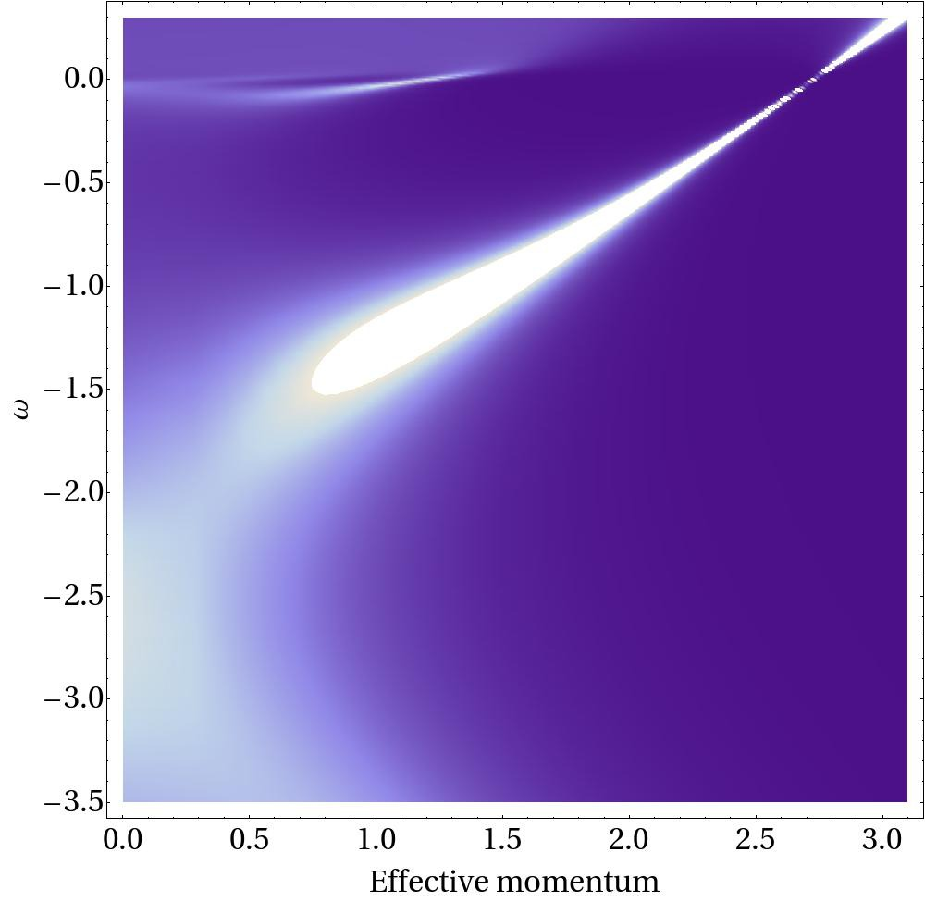 (B)
(B)
Collectively, the spectra in Fig. 2 show that conformality is only broken by the chemical potential and not by the magnetic field. Naively, the magnetic field introduces a new scale in the system. However, this scale is absent from the spectral functions, visually validating the the discussion in the previous section that the scale can be removed by a rescaling of the temperature and chemical potential.
One thus concludes that there is some value of the magnetic field, depending on , such that the spectral function loses its quasiparticle peaks and displays near-conformal behavior for . The nature of the transition and the underlying mechanism depends on the parameters . One mechanism, obvious from the rescaling in eq. (29), is the reduction of the effective coupling as increases. This will make the influence of the scalar potential negligible and push the system back toward conformality. Generically, the spectral function shows no sharp change but is more indicative of a crossover.
A more interesting phenomenon is the disappearance of coherent quasiparticles at high effective chemical potentials. For the special case , we can go beyond numerics and study this transition analytically, combining the exact solution found in [22] and the mapping (30). In the next section, we will show that the transition is controlled by the change in the dispersion of the quasiparticle and corresponds to a sharp phase transition. Increasing the magnetic field leads to a decrease in phenomenological control parameter . This can give rise to a transition to a non-Fermi liquid when , and finally to the conformal regime at when and the Fermi surface vanishes.
4.3 Density of states
As argued at the beginning of this section, the spectral function can look quite different depending on the particular basis chosen. Though the spectral function is an attractive quantity to consider due to connection with ARPES experiments, we will also direct our attention to basis-independent and manifestly gauge invariant quantities. One of them is the density of states (DOS), defined by
| (58) |
where the usual integral over the momentum is replaced by a sum since only discrete values of the momentum are allowed.
(A) (B)
(B)
In Fig. 4, we plot the density of states for two systems. We clearly see the Landau splitting of the Fermi surface. A peculiar feature of these plots is that the DOS seems to grow for negative values of . This, however, is an artefact of our calculation. Each individual spectrum in the sum eq. (58) has a finite tail that scales as for large , so each term has a finite contribution for large values of . When the full sum is performed, this fact implies that . The relevant information on the density of states can be obtained by regularizing the sum, which in practice is done by summing over a finite number of terms only, and then considering the peaks that lie on top of the resulting finite-sized envelope. The physical point in Fig. 4A is the linear spacing of Landau levels, corresponding to a non-relativistic system at finite density. This is to be contrasted with Fig. 4B where the level spacing behaves as , appropriate for a Lorentz invariant system and realized in graphene [25].
5 Fermi level structure at zero temperature
In this section, we solve the Dirac equation in the magnetic field for the special case (). Although there are no additional symmetries in this case, it is possible to get an analytic solution. Using this solution, we obtain Fermi level parameters such as and and consider the process of filling the Landau levels as the magnetic field is varied.
5.1 Dirac equation with
In the case , it is convenient to solve the Dirac equation including the spin connection (see details in [19]) rather than scaling it out:
where are the energies of the Landau levels , , is given by eq. (3), and the gamma matrices are defined in [19]. In this basis the two components and decouple. Therefore, in what follows we solve for the first component only (we omit index ). Substituting the spin connection, we have [18]:
| (62) |
with . It is convenient to change to the basis
| (63) |
which diagonalizes the system into a second order differential equation for each component. We introduce the dimensionless variables as in eqs. (15-17), and make a change of the dimensionless radial variable:
| (64) |
with the horizon now being at , and the conformal boundary at . Performing these transformations in eq. (62), the second order differential equations for reads
| (65) | |||||
The second component obeys the same equation with .
At ,
| (66) |
The solution of this fermion system at zero magnetic field and zero temperature has been found in [22]. To solve eq. (65), we use the mapping to a zero magnetic field system eq. (29). The combination at non-zero maps to at zero as follows:
| (67) |
where at we used . We solve eq. (65) for zero modes, i. e. , and at the Fermi surface , and implement eq. (67).
Near the horizon (, ), we have
| (68) |
which gives the following behavior:
| (69) |
with the scaling exponent following from eq. (32):
| (70) |
at the momentum . Using Maple, we find the zero mode solution of eq. (65) with a regular behavior at the horizon [22, 18]:
| (71) | |||||
and
| (72) | |||||
where is the hypergeometric function and are normalization factors. Since normalization factors are constants, we find their relative weight by substituting solutions given in eq. (71) back into the first order differential equations at ,
| (73) |
The same relations are obtained when calculations are done for any . The second solution , with behavior at the horizon, is obtained by replacing in eq.(71).
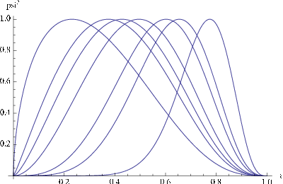
To get insight into the zero-mode solution (71), we plot the radial profile for the density function for different magnetic fields in Fig. (5). The momentum chosen is the Fermi momentum of the first Fermi surface (see the next section). The curves are normalized to have the same maxima. Magnetic field is increased from right to left. At small magnetic field, the zero modes are supported away from the horizon, while at large magnetic field, the zero modes are supported near the horizon. This means that at large magnetic field the influence of the black hole to the Fermi level structure becomes more important.
5.2 Magnetic effects on the Fermi momentum and Fermi velocity
In the presence of a magnetic field there is only a true pole in the Green’s function whenever the Landau level crosses the Fermi energy [23]
| (74) |
As shown in Fig. 2, whenever the equation (74) is satisfied the spectral function has a (sharp) peak. This is not surprising since quasiparticles can be easily excited from the Fermi surface. From eq. (74), the spectral function and the density of states on the Fermi surface are periodic in with the period
| (75) |
where is the area of the Fermi surface [23]. This is a manifestation of the de Haas-van Alphen quantum oscillations. At , the electronic properties of metals depend on the density of states on the Fermi surface. Therefore, an oscillatory behavior as a function of magnetic field should appear in any quantity that depends on the density of states on the Fermi energy. Magnetic susceptibility [23] and magnetization together with the superconducting gap [24] have been shown to exhibit quantum oscillations. Every Landau level contributes an oscillating term and the period of the -th level oscillation is determined by the value of the magnetic field that satisfies eq. (74) for the given value of . Quantum oscillations (and the quantum Hall effect which we consider later in the paper) are examples of phenomena in which Landau level physics reveals the presence of the Fermi surface. The superconducting gap found in the quark matter in magnetic fields [24] is another evidence for the existence of the (highly degenerate) Fermi surface and the corresponding Fermi momentum.
Generally, a Fermi surface controls the occupation of energy levels in the system: the energy levels below the Fermi surface are filled and those above are empty (or non-existent). Here, however, the association to the Fermi momentum can be obscured by the fact that the fermions form highly degenerate Landau levels. Thus, in two dimensions, in the presence of the magnetic field the corresponding effective Fermi surface is given by a single point in the phase space, that is determined by , the Landau index of the highest occupied level, i.e., the highest Landau level below the chemical potential 22 2 We would like to thank Igor Shovkovy for clarifying the issue with the Fermi momentum in the presence of the magnetic field.. Increasing the magnetic field, Landau levels ’move up’ in the phase space leaving only the lower levels occupied, so that the effective Fermi momentum scales roughly (excluding interactions) as a square root of the magnetic field, . High magnetic fields drive the effective density of the charge carriers down, approaching the limit when the Fermi momentum coincides with the lowest Landau level.
Many phenomena observed in the paper can thus be qualitatively explained by Landau quantization. As discussed before, the notion of the Fermi momentum is lost at very high magnetic fields. In what follows, the quantitative Fermi level structure at zero temperature, described by and values, is obtained as a function of the magnetic field using the solution of the Dirac equation given by eqs. (71,72). As in [11], we neglect first the discrete nature of the Fermi momentum and velocity in order to obtain general understanding. Upon taking the quantization into account, the smooth curves become combinations of step functions following the same trend as the smooth curves (without quantization). While usually the grand canonical ensemble is used, where the fixed chemical potential controls the occupation of the Landau levels [27], in our setup, the Fermi momentum is allowed to change as the magnetic field is varied, while we keep track of the IR conformal dimension .


The Fermi momentum is defined by the matching between IR and UV physics [7], therefore it is enough to know the solution at , where the matching is performed. To obtain the Fermi momentum, we require that the zero mode solution is regular at the horizon () and normalizable at the boundary. At the boundary , the wave function behaves as
| (76) |
To require it to be normalizable is to set the first term ; the wave function at is then
| (77) |
Eq. (77) leads to the condition , which, together with eq. (71), gives the following equation for the Fermi momentum as function of the magnetic field [22, 18]
| (78) |
with given by eq. (70). Using Mathematica to evaluate the hypergeometric functions, we numerically solve the equation for the Fermi surface, which gives effective momentum as if it were continuous, i.e. when quantization is neglected. The solutions of eq. (78) are given in Fig. (6). There are multiple Fermi surfaces for a given magnetic field . Here and in all other plots we choose , therefore , and . In Fig.(6), positive and negative correspond to the Fermi surfaces in the Green’s functions and . The relation between two components is [6], therefore Fig.(6) is not symmetric with respect to the x-axis. Effective momenta terminate at the dashed line . Taking into account Landau quantization of with , the plot consists of stepwise functions tracing the existing curves (we depict only positive ). Indeed Landau quantiaztion can be also seen from the dispersion relation at Fig. (3), where only discrete values of effective momentum are allowed and the Fermi surface has been chopped up as a result of it Fig. (3B).
Our findings agree with the results for the (largest) Fermi momentum in a three-dimensional magnetic system considered in [28], compare the stepwise dependence with Fig.(5) in [28].
In Fig.(7), the Landau level index is obtained from where is a numerical solution of eq. (78). Only those Landau levels which are below the Fermi surface are filled. In Fig.(6), as we decrease magnetic field first nothing happens until the next Landau level crosses the Fermi surface which corresponds to a jump up to the next step. Therefore, at strong magnetic fields, fewer states contribute to transport properties and the lowest Landau level becomes more important (see the next section). At weak magnetic fields, the sum over many Landau levels has to be taken, ending with the continuous limit as , when quantization can be ignored.
In Fig. (8), we show the IR conformal dimension as a function of the magnetic field. We have used the numerical solution for . Fermi liquid regime takes place at magnetic fields , while non-Fermi liquids exist in a narrow band at , and at the system becomes near-conformal.


In this figure we observe the pathway of the possible phase transition exhibited by the Fermi surface (ignoring Landau quantization): it can vanish at the line , undergoing a crossover to the conformal regime, or cross the line and go through a non-Fermi liquid regime, and subsequently cross to the conformal phase. Note that the primary Fermi surface with the highest and seems to directly cross over to conformality, while the other Fermi surfaces first exhibit a ”strange metal” phase transition. Therefore, all the Fermi momenta with contribute to the transport coefficients of the theory. In particular, at high magnetic fields when for the first (largest) Fermi surface is nonzero but small, the lowest Landau level becomes increasingly important contributing to the transport with half degeneracy factor as compared to the higher Landau levels.
In Fig. 9, we plot the Fermi momentum as a function of the magnetic field for the first Fermi surface (the largest root of eq. (78)). Quantization is neglected here. At the left panel, the relatively small region between the dashed lines corresponds to non-Fermi liquids . At large magnetic field, the physics of the Fermi surface is captured by the near horizon region (see also Fig. (5)) which is . At the maximum magnetic field, , when the black hole becomes pure magnetically charged, the Fermi momentum vanishes when it crosses the line . This only happens for the first Fermi surface. For the higher Fermi surfaces the Fermi momenta terminate at the line , Fig. (6). Note the Fermi momentum for the first Fermi surface can be almost fully described by a function . It is tempting to view the behavior as a phase transition in the system although it strictly follows from the linear scaling for by using the mapping (29). (Note that also .) Taking into account the discretization of , the plot will consist of an array of step functions tracing the existing curve. Our findings agree with the results for the Fermi momentum in a three dimensional magnetic system considered in [28], compare with Fig.(5) there.


The Fermi velocity given in eq. (27) is defined by the UV physics; therefore solutions at non-zero are required. The Fermi velocity is extracted from matching two solutions in the inner and outer regions at the horizon. The Fermi velocity as function of the magnetic field for is [22, 18]
| (79) |
where the zero mode wavefunction is taken at eq.(71).
We plot the Fermi velocity for several Fermi surfaces in Fig. 10. Quantization is neglected here. The Fermi velocity is shown for . It is interesting that the Fermi velocity vanishes when the IR conformal dimension is . Formally, it follows from the fact that [7]. The first Fermi surface is at the far right. Positive and negative correspond to the Fermi surfaces in the Green’s functions and , respectively. The Fermi velocity has the same sign as the Fermi momentum . At small magnetic field values, the Fermi velocity is very weakly dependent on and it is close to the speed of light; at large magnetic field values, the Fermi velocity rapidly decreases and vanishes (at for the first Fermi surface). Geometrically, this means that with increasing magnetic field the zero mode wavefunction is supported near the black hole horizon fig.(5), where the gravitational redshift reduces the local speed of light as compared to the boundary value. It was also observed in [22, 7] at small fermion charge values.

6 Hall and longitudinal conductivities
In this section, we calculate the contributions to Hall and the longitudinal conductivities directly in the boundary theory. This should be contrasted with the standard holographic approach, where calculations are performed in the (bulk) gravity theory and then translated to the boundary field theory using the AdS/CFT dictionary. Specifically, the conductivity tensor has been obtained in [10] by calculating the on-shell renormalized action for the gauge field on the gravity side and using the gauge/gravity duality to extract the charge current-current correlator at the boundary. Here, the Kubo formula involving the current-current correlator is used directly by utilizing the fermion Green’s functions extracted from holography in [7]. Therefore, the conductivity is obtained for the charge carriers described by the fermionic operators of the boundary field theory.
The use of the conventional Kubo formulo to extract the contribution to the transport due to fermions is validated in that it also follows from a direct AdS/CFT computation of the one-loop correction to the on-shell renormalized AdS action [15]. We study in particular stable quasiparticles with and at zero temperature. This regime effectively reduces to the clean limit where the imaginary part of the self-energy vanishes . We use the gravity-“dressed” fermion propagator from eq. (27) and to make the calculations complete, the “dressed” vertex is necessary, to satisfy the Ward identities. As was argued in [15], the boundary vertex which is obtained from the bulk calculations can be approximated by a constant in the low temperature limit. Also, according to [26], the vertex only contains singularities of the product of the Green’s functions. Therefore, dressing the vertex will not change the dependence of the DC conductivity on the magnetic field [26]. In addition, the zero magnetic field limit of the formulae for conductivity obtained from holography [15] and from direct boundary calculations [18] are identical.
6.1 Integer quantum Hall effect
Let us start from the “dressed” retarded and advanced fermion propagators [7]: is given by eq. (27) and . To perform the Matsubara summation we use the spectral representation
| (80) |
with the spectral function defined as . Generalizing to a non-zero magnetic field and spinor case [27], the spectral function [29] is
| (81) | |||||
where is the Fermi energy, is the energy of the Landau level, with spin projection operators , we take , the generalized Laguerre polynomials are and by definition , (we omit the vector part , it does not contribute to the DC conductivity), all ’s are the standard Dirac matrices, , and are real constants (we keep the same notations for the constants as in [7]). The self-energy contains the real and imaginary parts, . The imaginary part comes from scattering processes of a fermion in the bulk, e. g. from pair creation, and from the scattering into the black hole. It is exactly due to inelastic/dissipative processes that we are able to obtain finite values for the transport coefficients, otherwise they are formally infinite.
Using the Kubo formula, the DC electrical conductivity tensor is
| (82) |
where is the retarded current-current correlation function; schematically the current density operator is . Neglecting the vertex correction, it is given by
| (83) |
The sum over the Matsubara frequency is
| (84) |
Taking , the polarization operator is now
| (85) |
where the spectral function is given by eq. (81) and is the Fermi-Dirac distribution function. Evaluating the traces, we have
| (86) | |||||
with . We have also introduced with being the antisymmetric tensor (), and . In the momentum integral, we use the orthogonality condition for the Laguerre polynomials .
From eq. (86), the term symmetric/antisymmetric with respect to exchange contributes to the diagonal/off-dialgonal component of the conductivity (note the antisymmetric term ). The longitudinal and Hall DC conductivities () are thus
| (87) | |||||
where . The filling factor is proportional to the density of carriers: (see derivation in [19]). The degeneracy factor of the Landau levels is : for the lowest Landau level and for . Substituting the filling factor back to eq. (), the Hall conductivity can be written as
| (89) |
where is the charge density in the boundary theory, and both the charge and the magnetic field carry a sign (the prefactor comes from the normalization choice in the fermion propagator eqs. (27,81) as given in [7], which can be regarded as a factor contributing to the effective charge and is not important for further considerations). The Hall conductivity eq. (89) has been obtained using the AdS/CFT duality for the Lorentz invariant -dimensional boundary field theories in [10]. We recover this formula because in our case the translational invariance is maintained in the and directions of the boundary theory.
Low frequencies give the main contribution in the integrand of eq. (). Since the self-energy satisfies and we consider the regime , we have at (self-energy goes to zero faster than the term). Therefore, only the simple poles in the upper half-plane contribute to the conductivity where are small. The same logic of calculation has been used in [27]. We obtain for the longitudinal and Hall conductivities
| (90) | |||
| (91) |
where the Fermi energy is and the energy of the Landau level is . Similar expressions were obtained in [27]. However, in our case the filling of the Landau levels is controlled by the magnetic field through the field-dependent Fermi energy instead of the chemical potential .
At , and . Therefore the longitudinal and Hall conductivities are
| (92) | |||||
| (93) | |||||
where the Landau level index runs . It can be estimated as when ( denotes the integer part), with the average spacing between the Landau levels given by the Landau energy . Note that . We can see that eq. (93) expresses the integer quantum Hall effect (IQHE). At zero temperature, as we dial the magnetic field, the Hall conductivity jumps from one quantized level to another, forming plateaus given by the filling factor
| (94) |
with . (Compare to the conventional Hall quantization , that appears in thick graphene). Plateaus of the Hall conductivity at follow from the stepwise behavior of the charge density in eq.(89):
| (95) |
where Landau levels are filled and contribute to . The longitudinal conductivity vanishes except precisely at the transition point between the plateaus. In Fig. 11, we plot the longitudinal and Hall conductivities at , using only the terms after sign in eq. (91). In the Hall conductivity, plateau transition occurs when the Fermi level (in Fig. 11) of the first Fermi surface (Fig. 9) crosses the Landau level energy as we vary the magnetic field. By decreasing the magnetic field, the plateaus become shorter and increasingly more Landau levels contribute to the Hall conductivity. This happens because of two factors: the Fermi level moves up and the spacing between the Landau levels becomes smaller. This picture does not depend on the Fermi velocity as long as it is nonzero.
6.2 Fractional quantum Hall effect
In [19], using the holographic description of fermions, we obtained the filling factor at strong magnetic fields
| (96) |
where is the effective Landau level index. Eq.(96) expresses the fractional quantum Hall effect (FQHE). In the quasiparticle picture, the effective index is integer , but generally it may be fractional. In particular, the filling factors where have been proposed by Halperin [33] for the case of bound electron pairs, i.e. -charge bosons. Indeed, QED becomes effectively confining in ultraquantum limit at strong magnetic field, and the electron pairing is driven by the Landau level quantization and gives rise to bosons. In our holographic description, quasiparticles are valid degrees of freedom only for , i.e. for weak magnetic field. At strong magnetic field, poles of the fermion propagator should be taken into account in calculation of conductivity. This will probably result in a fractional filling factor. Our pattern for FQHE Fig.(11) resembles the one obtained by Kopelevich in Fig.3 [32] which has been explained using the fractional filling factor of Halperin [33].
The somewhat regular pattern behind the irregular behavior can be understood as a consequence of the appearance of a new energy scale: the average distance between the Fermi levels. For the case of Fig. 11, we estimate it to be with . The authors of [27] explain the FQHE through the opening of a gap in the quasiparticle spectrum, which acts as an order parameter related to the particle-hole pairing and is enhanced by the magnetic field (magnetic catalysis). Here, the energy gap arises due to the participation of multiple Fermi surfaces.
A pattern for the Hall conductivity that is strikingly similar to Fig.(11) arises in the AA and AB-stacked bilayer graphene, which has different transport properties from the monolayer graphene [31], compare with Figs.(2,5) there. It is remarkable that the bilayer graphene also exhibits the insulating behavior in a certain parameter regime. This agrees with our findings of metal-insulating transition in our system.


7 Conclusions
We have studied strongly coupled electron systems in the magnetic field focussing on the Fermi level structure, using the AdS/CFT correspondence. These systems are dual to Dirac fermions placed in the background of the electrically and magnetically charged AdS-Reissner-Nordström black hole. At strong magnetic fields the dual system ”lives” near the black hole horizon, which substantially modifies the Fermi level structure. As we dial the magnetic field higher, the system exhibits the non-Fermi liquid behavior and then crosses back to the conformal regime. In our analysis we have concentrated on the the Fermi liquid regime and obtained the dependence of the Fermi momentum and Fermi velocity on the magnetic field. Remarkably, exhibits the square root behavior, with staying close to the speed of light in a wide range of magnetic fields, while it rapidly vanishes at a critical magnetic field which is relatively high. Such behavior indicates that the system may have a phase transition.
The magnetic system can be rescaled to a zero-field configuration which is thermodynamically equivalent to the original one. This simple result can actually be seen already at the level of field theory: the additional scale brought about by the magnetic field does not show up in thermodynamic quantities meaning, in particular, that the behavior in the vicinity of quantum critical points is expected to remain largely uninfluenced by the magnetic field, retaining its conformal invariance. In the light of current condensed matter knowledge, this is surprising and might in fact be a good opportunity to test the applicability of the probe limit in the real world: if this behavior is not seen, this suggests that one has to include the backreaction to metric to arrive at a realistic description.
In the field theory frame, we have calculated the DC conductivity using and values extracted from holography. The holographic calculation of conductivity that takes into account the fermions corresponds to the corrections of subleading order in in the field theory and is very involved [15]. As we are not interested in the vertex renormalization due to gravity (it does not change the magnetic field dependence of the conductivity), we have performed our calculations directly in the field theory with AdS gravity-dressed fermion propagators. Instead of controlling the occupancy of the Landau levels by changing the chemical potential (as is usual in non-holographic setups), we have controlled the filling of the Landau levels by varying the Fermi energy level through the magnetic field. At zero temperature, we have reproduced the integer QHE of the Hall conductivity, which is observed in graphene at moderate magnetic fields. While the findings on equilibrium physics (Landau quantization, magnetic phase transitions and crossovers) are within expectations and indeed corroborate the meaningfulness of the AdS/CFT approach as compared to the well-known facts, the detection of the QHE is somewhat surprising as the spatial boundary effects are ignored in our setup. We plan to address this question in further work.
Interestingly, at large magnetic fields we obtain the correct formula for the filling factor characteristic for FQHE. Moreover our pattern for FQHE resembles the one obtained in [32] which has been explained using the fractional filling factor of Halperin [33]. In the quasiparticle picture, which we have used to calculate Hall conductivity, the filling factor is integer. In our holographic description, quasiparticles are valid degrees of freedom only at weak magnetic field. At strong magnetic field, the system exhibits non-Fermi liquid behaviour. In this case, the poles of the fermion propagator should be taken into account to calculate the Hall conductivity. This can probably result in a fractional filling factor. We leave it for future work.
Notably, the AdS-Reissner-Nordström black hole background gives a vanishing Fermi velocity at high magnetic fields. It happens at the point when the IR conformal dimension of the corresponding field theory is , which is the borderline between the Fermi and non-Fermi liquids. Vanishing Fermi velocity was also observed at high enough fermion charge [22]. As in [22], it is explained by the red shift on the gravity side, because at strong magnetic fields the fermion wavefunction is supported near the black hole horizon modifying substantially the Fermi velocity. In our model, vanishing Fermi velocity leads to zero occupancy of the Landau levels by stable quasiparticles that results in vanishing regular Fermi liquid contribution to the Hall conductivity and the longitudinal conductivity. The dominant contribution to both now comes from the non-Fermi liquid and conformal contributions. We associate such change in the behavior of conductivities with a metal-”strange metal” phase transition. Experiments on highly oriented pyrolitic graphite support the existence of a finite ”offset” magnetic field at where the resistivity qualitatively changes its behavior [30]. At , it has been associated with the metal-semiconducting phase transition [30]. It is worthwhile to study the temperature dependence of the conductivity in order to understand this phase transition better.
Acknowledgements.
The work was supported in part by the Alliance program of the Helmholtz Association, contract HA216/EMMI “Extremes of Density and Temperature: Cosmic Matter in the Laboratory” and by ITP of Goethe University, Frankfurt (E. Gubankova), by a VIDI Innovative Research Incentive Grant (K. Schalm) from the Netherlands Organization for Scientific Research (NWO), by a Spinoza Award (J. Zaanen) from the Netherlands Organization for Scientific Research (NWO) and the Dutch Foundation for Fundamental Research of Matter (FOM). K. Schalm thanks the Galileo Galilei Institute for Theoretical Physics for the hospitality and the INFN for partial support during the completion of this work.References
- (1) J. Zaanen, ”Quantum Critical Electron Systems: The Uncharted Sign Worlds”, Science 319, 1205 (2008); P. de Forcrand, ”Simulating QCD at finite density”, PoS LAT2009, 010 (2009), [arXiv:1005.0539 [hep-lat]].
- (2) S. A. Hartnoll, J. Polchinski, E. Silverstein and D. Tong, ”Towards strange metallic holography”, JHEP 1004, 120 (2010) [arXiv:0912.1061[hep-th]].
- (3) P. Kovtun, D. T. Son, A. O. Starinets, ”Viscosity in Strongly Interacting Quantum Field Theories from Black Hole Physics ”, Phys. Rev. Lett. 94, 111601 (2005), [arXiv:0405231[hep-th]].
- (4) S. -S. Lee, ”A non-Fermi liquid from a charged black hole: a critical Fermi ball”, Phys. Rev. D 79, 086006 (2009) [arXiv:0809.3402[hep-th]].
- (5) M. Čubrović, J. Zaanen and K. Schalm, ”String theory, quantum phase transitions and the emergent Fermi-liquid”, Science 325, 439 (2009) [arXiv:0904.1993[hep-th]].
- (6) H. Liu, J. McGreevy and D. Vegh, ”Non-Fermi liquids from holography”, arXiv:0903.2477 [hep-th].
- (7) T. Faulkner, H. Liu, J. McGreevy and D. Vegh, ”Emergent quantum criticality, Fermi surfaces, and AdS2”, [arXiv:0907.2694 [hep-th]].
- (8) S. A. Hartnoll and A. Tavanfar, ”Electron stars for holographic metallic criticality”, [arXiv:1008.2828[hep-th]].
- (9) S. A. Hartnoll, P. K. Kovtun, M. Mueller and S. Sachdev, ”Theory of the Nernst effect near quantum phase transitions in condensed matter, and in dyonic black holes”, Phys. Rev. B 76, 144502 (2007) [arXiv:0706.3215[hep-th]].
- (10) S. A. Hartnoll and P. Kovtun, ”Hall conductivity from dyonic black holes”, Phys. Rev. D 76, 066001 (2007), [arXiv:0704.1160[hep-th]].
- (11) P. Basu, J. Y. He, A. Mukherjee and H.-H. Shieh, ”Holographic Non-Fermi Liquid in a Background Magnetic Field”, [arXiv:10908.1436[hep-th]].
- (12) T. Albash and C. V. Johnson, ”Landau Levels, Magnetic Fields and Holographic Fermi Liquids”, J. Phys. A: Math. Theor. 43, 345404 (2010) [arXiv:1001.3700[hep-th]]; T. Albash and C. V. Johnson, ”Holographic Aspects of Fermi Liquids in a Background Magnetic Field”, J. Phys. A: Math. Theor. 43, 345405 (2010) [arXiv:0907.5406[hep-th]].
- (13) T. Albash and C. V. Johnson, ”A holographic superconductor in an external magnetic field”, JHEP 0809, 121 (2008) [arXiv:0804.3466[hep-th]].
- (14) N. Iqbal, H. Liu, M. Mezei and Q. Si ”Quantum phase transitions in holographic models of magnetism and superconductors”, [arXiv:1003.0010[hep-th]].
- (15) T. Faulkner, N. Iqbal, H. Liu, J. McGreevy and D. Vegh, ”From black holes to strange metals”, [arXiv:1003.1728[hep-th]].
- (16) E. D’Hoker and P. Kraus, JHEP 1005, 083 (2010) [arXiv:1003.1302 [hep-th]].
- (17) A. Auerbach, ”Quantum Magnetism Approaches to Strongly Correlated Electrons ”, [arXiv:cond-mat/9801294].
- (18) E. Gubankova, ”Particle-hole instability in the holography”, [arXiv:1006.4789[hep-th]].
- (19) E. Gubankova, J. Brill, M. Cubrovic, K. Schalm, P. Schijven, J. Zaanen, ”Holographic fermions in external magnetic fields”, Phys. Rev. D 84, 106003 (2011), [arXiv:1011.4051[hep-th]].
- (20) J. L. Davis, P. Kraus and A. Shah, ”Gravity Dual of a Quantum Hall Plateau Transition”, JHEP 0811, 020 (2008) [arXiv:0809.1876[hep-th]]; E. K. -Vakkuri, P. Kraus, ”Quantum Hall Effect in AdS/CFT”, JHEP 0809, 130 (2008) [arXiv:0805.4643[hep-th]].
- (21) A. H. MacDonald, ”Introduction to the physics of the Quantum Hall regime”, [arXiv:cond-mat/9410047].
- (22) T. Hartman and S. A. Hartnoll, ”Cooper pairing near charged black holes”, [arXiv:1003.1918[hep-th]].
- (23) F. Denef, S. A. Hartnoll and S. Sachdev, ”Quantum oscillations and black hole ringing”, arXiv:0908.1788 [hep-th]; F. Denef, S. A. Hartnoll and S. Sachdev, ”Black hole determinants and quasinormal modes”, arXiv:0908.2657 [hep-th].
- (24) J. L. Noronha, I. A. Shovkovy, ”Color-flavor locked superconductor in a magnetic field”, Phys. Rev. D 76,105030 (2007) [arXiv:0708.0307[hep-ph]].
- (25) Y. Zhang, Z. Jiang, J. P. Small, M. S. Purewal, Y.-W. Tan, M. Fazlollahi, J. D. Chudow, J. A. Jaszczak, H. L. Stormer and P. Kim, ”Landau Level Splitting in Graphene in High Magnetic Fields”, Phys. Rev. Lett. 96, 136806 (2006) [arXiv:0602649[cond-mat]].
- (26) M. A. V. Basagoiti, ”Transport coefficients and ladder summation in hot gauge theories”, Phys. Rev. D 66, 045005 (2002) [arXiv:hep-ph/0204334]; J. M. M. Resco, M. A. V. Basagoiti, ”Color conductivity and ladder summation in hot QCD”, Phys. Rev. D 63, 056008 (2001), [arXiv:hep-ph/0009331].
- (27) V. P. Gusynin and S. G. Sharapov, ”Transport of Dirac quasiparticles in graphene: Hall and optical conductivities”, Phys. Rev. B 73, 245411 (2006) [arXiv:0512157[cond-mat]].
- (28) E. V. Gorbar, V. A. Miransky, I. A. Shovkovy, ”Dynamics in the normal ground state of dense relativistic matter in a magnetic field”, [arXiv:1101.4954[hep-th]].
- (29) N. Iqbal and H. Liu, ”Real-time response in AdS/CFT with application to spinors”, Fortsch. Phys. 57, 367 (2009), [arXiv:0903.2596[hep-th]].
- (30) Y. Kopelevich, V. V. Lemanov, S. Moehlecke and J. H. S. Torrez, ”Landau Level Quantization and Possible Superconducting Instabilities in Highly Oriented Pyrolitic Graphite”, Fiz.Tverd.Tela 41, 2135 (1999) [Phys. Solid State 41, 1959 (1999)]; H. Kempa, Y. Kopelevich, F. Mrowka, A. Setzer, J. H. S. Torrez, R. Hoehne and P. Esquinazi, Solid State Commun. 115, 539 (2000); M. S. Sercheli, Y. Kopelevich, R. R. da Silva, J. H. S. Torrez and C. Rettori, Solid State Commun. 121, 579 (2002); Y. Kopelevich, P. Esquinazi, J. H. S. Torres, R. R. da Silva, H. Kempa, F. Mrowka, R. Ocana, ”Metal-Insulator-Metal Transitions, Superconductivity and Magnetism in Graphite”, Studies of H-Temp. Supercond. 45, 59 (2003), [arXiv:0209442 [cond-mat]].
- (31) Y.-F. Hsu, G.-Y. Guo, ”Anomalous integer quantum Hall effect in AA-stacked bilayer graphene”, Phys. Rev. B 82, 165404 (2010), [arXiv:1008.0748[cond-mat]].
- (32) Y. Kopelevich, B. Raquet, M. Goiran, W. Escoffier, R. R. da Silva, J. C. Medina Pantoja, I. A. Luk’yanchuk, A. Sinchenko, and P. Monceau, ”Searching for the fractional quantum Hall effect in graphite”, Phys. Rev. Lett. 103 116802 (2009).
- (33) B. I. Halperin, Helv. Phys. Acta 56 75 (1983).