SRG/eROSITA prospects for the detection of stellar tidal disruption flares

The flux decay of TDE flares is broadly consistent with a power law with a slope of $\sim-5/3$ (Komossa, 2002; Halpern, Gezari, & Komossa, 2004; Vaughan, Edelson, & Warwick, 2004). This decay probably reflects the decreasing accretion rate, $\dot{M}$, of the falling back stellar material by the SMBH, coupled with some constant radiative efficiency $\epsilon$ (the source luminosity $L=\epsilon\dot{M}c^{2}$), since the viscous timescale is believed to be shorter than the characteristic dynamical fallback time (Rees, 1988; Phinney, 1989). However, Lodato et al. (2009) found that a $t^{-5/3}$ decrease of $\dot{M}$ is reached only asymptotically at late times, while at earlier stages the behavior of the accretion rate is sensitive to the structure of the disrupted star. Besides that, the radiative efficiency of accretion is probably constant only at a certain phase of the event, namely when $\dot{M}$ is below the critical value $\dot{M}_{Edd}=\epsilon^{-1}L_{Edd}/c^{2}$ corresponding to the Eddington luminosity $L_{Edd}\backsimeq 1.3\times 10^{44}\left(\frac{M_{BH}}{10^{6}M_{☉}}\right)$ erg s^-1, but still above $\sim 0.01\dot{M}_{Edd}$. At this stage, the released gravitational energy is radiated away by a geometrically thin, optically thick accretion disk (Shakura & Sunyaev, 1973). For a solar type star with a peri-center distance $R_{p}=3R_{S}$ (where $R_{S}$ is the Schwarzschild radius), the peak mass rate occurs at time

$$\tau_{i}\backsimeq 20\left(\frac{M_{BH}}{10^{6}M_{☉}}\right)^{5/2}~{\rm min}$$

(1)

after the instant of disruption $t_{0}$ and is highly supercritical given $\epsilon=0.1$ and $M_{BH}\lesssim 10^{7}M_{☉}$ (Strubbe & Quataert 2009; this delay is in fact highly sensitive to pericenter distance: $\tau_{i}\propto R_{p}^{3}$). Therefore, early on accretion takes place in radiatively inefficient regime, with an approximately constant luminosity $L\backsimeq L_{Edd}$ emitted by a thick accretion disk, which is likely subject to outflows (Ulmer, 1999; Strubbe & Quataert, 2009). The boundary between the early (Eddington) and late (decay) phases lies at

$$\tau_{Edd}\backsimeq 0.1\left(\frac{M_{BH}}{10^{6}M_{☉}}\right)^{2/5}~{\rm yr}$$

(2)

after disruption for $R_{p}=3R_{S}$ ($\tau_{Edd}\propto R_{p}^{6/5}$, Strubbe & Quataert 2009). Although the reality can be somewhat more complicated (see e.g. Lodato et al. 2009), we adopt the following approximate relation for the time profile of flares associated with TDEs:

$$L(t)=\left\{\begin{array}[]{ll}L_{quies}&{\rm for}~\ t<t_{0}\\ L_{0}&{\rm for}~t_{0}<t<t_{1}\\ L_{0}\left(\frac{t-t_{0}}{\tau_{Edd}}\right)^{-5/3}&{\rm for}~t>t_{1}\end{array}\right.$$

(3)

where $L_{quies}$ is the source luminosity in the quiescent state, $L_{0}=\eta L_{Edd}\gg L_{quies}$ is the peak observed luminosity (with $\eta$ being a geometrical dilution factor), and $t_{1}=t_{0}+\tau_{Edd}$. Equation (3) ignores the short period $\tau_{i}\ll\tau_{Edd}$ since $\tau_{i}/{\tau_{Edd}}\simeq 4\times 10^{-4}\left({M_{BH}}/{10^{6}M_{☉}}\right)^{21/10}\left({R_{p}}/{3R_{S}}\right)^{9/5}$. However, as we further discuss in Section 4.2 below, there is an interesting possibility to observe some TDEs during the rising phase of the flare, which lasts $\tau_{rise}<\tau_{i}\ll\tau_{Edd}$ (under our assumption of shortness of the viscous time compared to the fallback time) and can be significantly long for large $M_{BH}$ and/or $R_{p}$.

For SMBHs with $M_{BH}\gtrsim{\rm few}\times 10^{7}M_{☉}$, only the closest stellar disruptions (small $R_{p}$) can lead to supercritical accretion, while the majority of TDE flares associated with such SMBHs are expected to be sub-Eddington (given a uniform distribution of pericenters, Ulmer 1999). Moreover, most of the emission will appear at UV rather than X-ray energies (see Section 2.2 below). We thus restrict our consideration to SMBHs with $M_{BH}\lesssim 10^{7}M_{☉}$.

We note that very recent analytic (Stone, Sari, & Loeb, 2012) and numerical (Guillochon & Ramirez-Ruiz, 2013) calculations indicate that the characteristic timescales discussed above might be almost independent of $R_{p}$, since the stellar debris energy ’freezes in’ at the tidal radius $R_{t}=R_{\star}\left(M_{BH}/M_{\star}\right)^{1/3}$ (where $R_{\star}$ and $M_{\star}$ are the mass and radius of the disrupted star), rather than at $R_{p}$ as was thought before (see Stone, Sari, & Loeb 2012 for a thorough discussion). The resulting difference is small for $M_{BH}=10^{7}M_{☉}$ (since $R_{t}/3R_{S}=1.6$, assuming $R_{\star}=R_{☉}$ and $M_{\star}=M_{☉}$), but becomes significant for lighter SMBHs, since $R_{t}/3R_{S}=7.5$ for $M_{BH}\sim 10^{6}M_{☉}$, which should lead to longer $\tau_{i}$ and $\tau_{Edd}$ and hence to slower flux decay during the post-peak phase. However, there is no observational confirmation of these new theoretical results yet. Furthermore, the TDE light curves observed so far are consistent with the shorter decay time-scales expected for $R_{p}\sim 3R_{S}$ (Esquej et al., 2008). Since we make our predictions for the eROSITA TDE detection rate (in Section 4) using the same (currently available) data set, we shall for simplicity assume $R_{p}=3R_{S}$.

An observer will detect only a fraction of the TDE bolometric flux, depending on the spectral energy distribution of TDE emission and the energy response of the detector used. Since this emission presumably originates in an accretion disk around a SMBH, its spectral energy distribution can be approximated (Shakura & Sunyaev, 1973) by a black body radiation spectrum with temperature

$$\kappa T_{bb}\simeq 0.06\left(\frac{M_{BH}}{10^{6}M_{\odot}}\right)^{-1/4}\left(\frac{\dot{M}}{\dot{M_{Edd}}}\right)^{1/4}\,{\rm keV},$$

(4)

which corresponds to the innermost regions of the disk ($R\sim 5R_{S}$, Ulmer 1999). Since this emission is fairly soft, the detection probability must strongly depend on the absorption column density to the source, implying that X-ray selected samples might be biased against absorbed TDE events. No indication of significant intrinsic absorption has been found from spectral analysis performed for known TDE candidates under the assumption of black body emission. The estimated black body temperatures are $\kappa T_{bb}\simeq 0.07$ keV (the median value, Komossa 2002; Esquej et al. 2008), although the quality of the existing X-ray data hardly makes it possible to distinguish a black body model from e.g. an absorbed power-law model (Esquej et al., 2008). Power-law fits typically resulted in steep slopes ($\Gamma\gtrsim 3$), i.e. the observed spectra are indeed soft.

Disregarding the remaining uncertainty in the spectral shape of TDE emission, we use the (physically motivated) absorbed black body model in our calculations. This model has 3 parameters: absorption column density $N_{H}$, temperature $\kappa T_{bb}$ and peak bolometric flux

$$f_{0}=\frac{L_{0}}{4\pi d_{L}^{2}},$$

(5)

where $d_{L}$ is the luminosity distance to the source (see Section 4). We freeze the first parameter at $N_{H}=5\times 10^{20}$ cm^-2, which is close to the median value of Galactic absorption for random positions in the extragalactic sky as calculated by Esquej et al. (2008). In addition to the Galactic absorption there might also be some intrinsic absorption due to edge-on orientation of the accretion disk and/or screening by unbound stellar debris material (Strubbe & Quataert, 2009). However, in the former case the disk radiation might be directed preferentially away from the observer, and so the contribution of such events to the net detection rate is likely to be small. In the latter case, the estimates of Strubbe & Quataert (2009) indicate that unbound equatorial material builds up a ’vertical wall‘ of debris with huge column density in the radial direction but subtending a small solid angle $\Delta\Omega\sim 0.1$ sr. Such screening will most likely result in complete non-detection rather than detection of a TDE with a significant excess of absorption relative to the Galactic value.

As follows from Eq. 4, the second parameter of the model obeys $\kappa T_{bb}\propto M_{BH}^{-1/4}$. Unfortunately, there are only crude $M_{BH}$ estimates for known TDE candidates. The median observed temperature $\kappa T_{bb}\simeq 0.07$ keV implies a SMBH with mass $M_{BH}\approx 10^{6}M_{\odot}$. For comparison, for $M_{BH}=5\times 10^{6}$ and $10^{7}M_{\odot}$ one expects $\kappa T_{bb}=0.047$ and $0.039$ keV, respectively. We shall use these three fiducial values in our calculations.

As the accretion rate of falling back material decreases, the effective temperature of the radiation is also expected to decrease as $\kappa T_{bb}\propto\dot{M}^{1/4}$, as long as the thin disk approximation remains valid (Strubbe & Quataert, 2009). Nonetheless, late observations of five TDE candidates from RASS (Vaughan, Edelson, & Warwick, 2004) demonstrated no significant softening and in fact indicated a marginal hardening for some of them, while the luminosities fell by more than two orders of magnitude⁴⁴ 4 It should be mentioned that the host galaxies of some of these candidates are classified as hosting an active nucleus.; Komossa et al. (2004) found similar spectral hardening for another TDE candidate, RX J1242–1119. This behavior may have resulted from transition to a different accretion mode accompanied by Comptonization of disk radiation in a hot corona and/or significant contribution from a relativistic jet. Taking into account these observations and because we expect eROSITA to detect TDEs mostly during an early post-peak phase (see Section 4), we disregard possible spectral evolution of TDE-associated emission in our estimates below.

It is also worth mentioning that somewhat higher temperatures ($\kappa T_{bb}\sim 0.12$ keV) have been reported for TDE candidates detected in clusters of galaxies (Cappelluti et al., 2009; Maksym, Ulmer, & Eracleous, 2010). It is unclear whether this is owing to some selection bias, the specific physical environment and/or details of the spectral analysis. In any case, searches for TDE candidates with eROSITA in galaxy clusters will be challenging due to the strong diffuse X-ray emission from the hot intracluster gas (which is much less of an issue for Chandra, Maksym, Ulmer, & Eracleous 2010), except for brightest flares in nearby clusters (like the one reported by Cappelluti et al. 2009), for which elaborate spectral analyses can be performed taking advantage of eROSITA’s higher sensitivity below 0.3 keV compared to Chandra. A further advantage in studying such events might be that galaxy clusters belong to the main scientific targets of eRASS (Merloni et al., 2012) and will thus be extensively covered by follow-up observations.

The SRG satellite will be rotating with a period of $T=4$ hours around its axis pointed within a few degrees of the Sun, with the telescopes observing the sky at right angles to the axis (Merloni et al., 2012). Following the orbit of the L2 point around the Sun the rotation axis will be moving at a speed of 1 deg per day. With the 1 deg-diameter field of view (FoV), eROSITA will complete an all-sky survey every 6 months and a total of 8 scans will be performed over the course of the mission. A typical position on the sky will receive $\sim 240$ seconds of exposure during one scan. This exposure will be achieved by 6 consecutive passages of a source through the eROSITA FoV separated by $\sim 4$-hour intervals (see Khabibullin, Sazonov, & Sunyaev 2012 for further details). A typical visit of a point source will thus last $\sim 1$ day, which is much shorter than the expected characteristic timescale of the flux decay during a TDE flare (few months). Hence, we shall regard such visits as single 240 s-long observations.

We note that in reality the eRASS exposure is not constant over the sky and increases with ecliptic latitude. Most importantly, there are two areas of $\sim 1000$ deg² each, surrounding the ecliptic poles, that will be visited more than 20 times during each eROSITA all-sky scan (Merloni et al., 2012). Hence, the threshold for detecting TDE flares in these regions will be $\sim 4$ times lower than the all-sky average used in our analysis below. That will not only allow one to detect weaker TDE flares (including events from more distant galaxies) but also to study in greater detail the X-ray light curves of bright TDE flares. This can be particularly important for detecting TDEs during their rise phase (See Section 4.2).

For a TDE with a given spectral energy distribution, bolometric flux $f$ (see Subsection 2.2) and redshift $z$, the count rate measured by eROSITA between 0.2 and 2 keV can be written as

$$C_{0.2-2}(f,z)=\frac{A_{0.2-2}}{K_{0.2-2}\left(z\right)}f,$$

(6)

where $A_{0.2-2}$ (in units of counts cm²/erg) is the flux-to-count conversion factor for a TDE at $z\to 0$ and the correcting factor $K_{0.2-2}\left(z\right)$ accounts for the cosmological reddening of the spectrum. Both $A_{0.2-2}$ and $K_{0.2-2}$ depend on the eROSITA response matrix and TDE spectrum. We have computed the redshift correction for different relevant spectral models using XSPEC (Dorman & Arnaud, 2001), and it proves to be significant (see Fig. 4), especially for the model corresponding to $M_{BH}=10^{7}M_{\odot}$. This has an obvious explanation: as the intrinsic TDE spectrum becomes softer with increasing black hole mass, a largely fraction of the photons red-shift out of the eROSITA energy band into softer bands (below 0.2 keV).

Disregarding spectral evolution during the TDE, the count rate varies with time as $C_{0.2-2}(t_{observer})\varpropto L\left(t_{source}(t_{observer})\right)$, where the relation $t_{source}(t_{observer})$ is governed by the source’s redshift.

Additional information on the nature of TDE candidates can be obtained by dividing the 0.2–2 keV energy band into several sub-bands, e.g. 0.2–0.4, 0.4–1 and 1–2 keV. The first one is sensitive to absorption along the line of sight, whereas the other two are well suited for estimating the effective spectral slope. We thus introduce a softness ratio $SR=C_{0.4-1}/C_{1-2}$ to distinguish ’soft‘ and ’hard‘ sources (see Appendix for further details).

Taking into account the anticipated TDE properties (see Section 2) and eRASS characteristics (see Section 3.1), we propose to discriminate TDEs against other types of X-ray transients to be detected during the survey (such as AGN flares and GRB afterglows, see e.g. Komossa 2002) based on the following two signatures:

• •

  large ($\geq 10$) variation between the count rates ($C_{0.2-2}$) measured in two consequent half-a-year scans (see Fig. 2);

• •

  soft spectrum (as indicated by the softness ratio $SR$), consistent with a weakly absorbed ($N_{H}<10^{21}$ cm^-2) power law with a photon index $\Gamma\geq 3$.

In addition, since we are dealing with soft X-ray flares, it is reasonable to limit TDE searches to Galactic latitudes $|b|>30^{\circ}$, where interstellar absorption $N_{H}<10^{21}$ cm^-2. That will also minimize contamination from cataclysmic variables and flaring dM stars, whose appearance can resemble TDEs (see Donley et al. 2002).

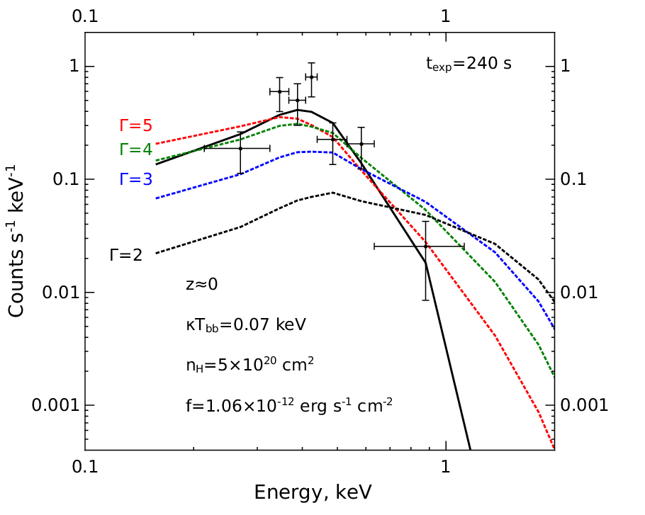
Although the peak X-ray flux during a TDE can greatly exceed the corresponding quiescent flux, i.e. the flux produced by the TDE’s host galaxy, in reality the minimum flux will, in most cases, be dominated by the eROSITA background (see Appendix). Therefore, the first of our requirements formulated above implies that a candidate TDE must be at least 10 times as bright as the background. Besides that, the count rate must be high enough for the softness ratio $SR$ to indicate that $\Gamma>3$ rather than $\Gamma\sim 2$ as typical of AGN. As demonstrated in Appendix, these conditions imply that at least $N_{lim}=40$ counts (i.e. 20 counts inside the half power diameter region) must be collected from a source between 0.2 and 2 keV during a 240 s exposure. The corresponding bolometric flux limits $f_{lim}$ for various spectral models are given in Table 2. Figure 6 shows a simulated eROSITA spectrum (for $M_{BH}=10^{6}M_{\odot}$) of a TDE with $f=f_{lim}$. Trial fits of this spectrum by various characteristic models demonstrate that it is feasible to reveal the spectral softness of a TDE using $\sim 40$ counts.

We can finally formulate exact criteria that can be used for identification of TDE candidates during eRASS:

1. 1.

   Extragalactic ($|b|>30^{\circ}$) location.

2. 2.

   At least 40 counts (or 20 counts inside the half power diameter region) detected from the source during the $\sim 240$ s exposure in a given scan of the sky.

3. 3.

   At least a factor of 10 higher count rate in comparison with the preceding or succeeding scan.

4. 4.

   Softness ratio $SR\geq 2$ in the bright state.

The last criterion should not be used in application to relativistic TDEs, a subclass of TDEs discussed in Section 4.4 below.

A TDE X-ray flare discovered in a given eRASS scan can remain detectable by eROSITA in its subsequent sky scans, i.e. 6 months, 12 months etc. after the TDE trigger. This provides an interesting possibility of obtaining a crude (2 or more data points) long-term light curve of TDE emission. Specifically, to obtain a significant (see Appendix for details) X-ray detection from a continuing TDE flare (whose position is known from its initial observation by eROSITA), just $\sim 4$ counts during the $\sim 240$ s exposure are required. This implies, for instance, that a TDE flare will be detectable by eROSITA even if the X-ray flux has dropped by an order of magnitude during 6 months after the trigger. Such late detections, or even upper limits provided by non-detections, will be very useful for testing TDE models.

We assume $\Lambda CDM$ cosmology with $\Omega_{M}=0.275,\Omega_{\Lambda}=0.725$ and $h=0.7$ (Komatsu et al., 2011). The luminosity distance as a function of redshift is then given by

$$d_{L}\left(z\right)=\left(1+z\right)d_{H}~\int_{0}^{z}\frac{dz^{\prime}}{E\left(z^{\prime}\right)},$$

(7)

where $d_{H}=\frac{c}{H_{0}}\approx 3.0h^{-1}$ Gpc $\approx 4.3$ Gpc is the Hubble distance, and $E\left(z\right)=\sqrt{\Omega_{m}\left(1+z\right)^{3}+\Omega_{\Lambda}}$ (Hogg, 1999). Defining $J\left(z\right)=\int_{0}^{z}\frac{dz^{\prime}}{E\left(z^{\prime}\right)}$, equation (7) becomes $d_{L}\left(z\right)=d_{H}\left(1+z\right)J\left(z\right)$.

Given the flux detection limit $f_{lim}$ corresponding to a given spectral model (Table 2), there exists the largest distance $d_{L,lim}$ (or the corresponding redshift $z_{lim}$) from which a TDE flare at its peak could be identified with eROSITA:

$$\frac{L_{0}}{4\pi d_{L}\left(z_{lim}\right)^{2}K\left(z_{lim}\right)}=f_{lim}$$

(8)

or

$$\left(1+z_{lim}\right)^{2}J\left(z_{lim}\right)^{2}K\left(z_{lim}\right)=\frac{L_{0}}{4\pi d_{H}^{2}f_{lim}}.$$

(9)

Solving this equation numerically with $L_{0}=1.3\times 10^{44}$ erg s^-1 (the Eddington luminosity for a black hole with mass $M_{BH}=10^{6}M_{\odot}$ and geometrical dilution factor $\eta=1$), we obtain $z_{lim}=0.164$. This is approximately two times further than the distance within which TDEs could be found with RASS ($z\approx 0.09$, Donley et al. 2002; Esquej et al. 2008). Similar calculations for $M_{BH}=5\times 10^{6}$ and $10^{7}M_{\odot}$, again assuming the Eddington luminosity at the peak phase, result in $z_{lim}=0.162$ and 0.142, respectively. Remarkably, the limiting redshifts for the different SMBH masses prove to be similar. This happens because although the peak TDE bolometric luminosity increases with $M_{BH}$, the spectrum becomes softer and most of the emission appears at frequencies below the eROSITA energy range.

Consider now a small volume of the Universe at redshift $z$ with radial width $dz$, covering an opening angle $\omega$ on the observer’s sky. The comoving volume of the slice is

$$dV_{c}\left(z\right)=\omega d_{H}^{3}\frac{J\left(z\right)^{2}}{E\left(z\right)}dz$$

(10)

(Hogg 1999; see also Chapter 13 of Peebles 1993). Neglecting any evolutionary changes in the galaxy population between $z_{lim}$ and $z=0$, we can calculate the rate of TDEs in this volume as $d\mathcal{N}\left(z\right)=\mathcal{R}dV_{c}\left(z\right)dt$.

Taking into account both the maximum and decay phases of the light curve (eq. (3)), a TDE flare remains detectable during a comoving time

$$\tau_{lim}\left(z\right)=\tau_{Edd}\left(\frac{L_{0}}{4\pi d_{H}^{2}f_{lim}}\frac{1}{\left(1+z\right)^{2}J\left(z\right)^{2}K\left(z\right)}\right)^{3/5}.$$

(11)

Hence, at a given moment of observation there are

$$d\mathcal{N}\left(z\right)=\mathcal{R}\times\tau_{lim}\left(z\right)\times dV_{c}\left(z\right)$$

(12)

detectable TDEs. Substituting the corresponding expressions for $dV_{c}\left(z\right)$ and $\tau_{lim}\left(z\right)$ and integrating from $z=0$ to $z_{lim}$, we obtain the total number of detectable TDEs:

$$\mathcal{N}=\alpha\times I(z_{lim}),$$

(13)

where

$$\alpha=\omega\mathcal{R}d_{H}^{3}\tau_{Edd}\left(\frac{L_{0}}{4\pi d_{H}^{2}f_{lim}}\right)^{3/5}$$

(14)

and

$$I(z_{lim})=\int_{0}^{z_{lim}}\frac{K\left(z\right)^{-3/5}J\left(z\right)^{4/5}}{\left(1+z\right)^{6/5}~E\left(z\right)}dz.$$

(15)

Finally, expressed in convenient units, the total number of detectable TDEs at a given moment is

$$\mathcal{N}\simeq 9.51\times 10^{4}\left(\frac{\omega}{2\pi}\right)\left(\frac{\mathcal{R}}{10^{-5}}\right)\left(\frac{\tau_{Edd}}{0.1}\right)\left(\frac{L_{0}}{10^{44}}\right)^{3/5}\left(\frac{f_{lim}}{10^{-12}}\right)^{-3/5}I\left(z_{lim}\right).$$

(16)

Estimates of the SMBH mass function (Hopkins, Richards, & Hernquist, 2007; Greene & Ho, 2007) indicate that the spatial density of SMBHs is roughly constant in the mass range from $\sim 10^{6}$ to $10^{7}M_{\odot}$ but depends on redshift. The TDE rate may demonstrate some correlation (Brockamp, Baumgardt, & Kroupa, 2011) or anti-correlation (Wang & Merritt, 2004) with the central SMBH mass. Therefore, since the maximum TDE distance for eRASS is almost independent of SMBH mass, we may expect the TDEs found during eRASS to be distributed over the $M_{BH}$ range from $\sim 10^{6}$ to $\sim 10^{7}M_{\odot}$. Since this distribution is currently unknown, we consider three different scenarios in which all TDEs detected during eRASS are characterized by a fixed $M_{BH}$ value: $10^{6}$, $5\times 10^{6}$ or $10^{7}M_{\odot}$. The resulting estimates are summarized in Table 2.

For $M_{BH}=10^{6}M_{\odot}$ and adopting $\mathcal{R}=5\times 10^{-6}$ yr^-1 Mpc^-3, $\omega=2\pi$ (which corresponds to the $|b|>30^{\circ}$ sky) and $R_{p}=3R_{S}$, we find from equations (2) and (15) that $\tau_{Edd}=0.1$ yr and $I\left(z_{lim}\right)\approx\frac{1}{4.5}z_{lim}^{1.5}=0.0153$, and finally from equation (16) that $\mathcal{N}\approx 650$ events can be discovered in the second eRASS scan through comparison with the first one. Figure 8 shows the distribution of the TDE flares over redshift and as a function of time passed after stellar destruction. Approximately half of the TDE triggers are expected to take place during the supercritical accretion phase. For $\sim 1/12$ of the events, a second trigger (during the subsequent eRASS scan) will be possible, and in rare cases, three or more independent triggers will be possible. Thus, the majority of TDEs will be ‘new’ for each scan, i.e. not seen during the preceding one. For $M_{BH}=5\times 10^{6}$ and $10^{7}M_{\odot}$, the fraction of ‘old’ TDEs, i.e. events observed in more than one eRASS scan is higher (Fig. 10 and Fig. 12) since the characteristic decay time positively correlates with the black hole mass (see Section 2).

Besides that, it turns out that the majority of TDEs discovered in a given eRASS scan will still be detectable (i.e. significantly exceeding the background flux level) by eROSITA (see Section 3.3) in the subsequent sky scan(s), i.e. 6 months, 12 months etc. after the initial trigger. Hence, eROSITA will typically provide 2–4 significant data points for constructing a long-term X-ray light curve of a TDE flare (see Table 2 and Figs. 8–12). As a result, eRASS will provide a unique sample of TDE light curves, which can be used to test TDE models.

The above estimates were based on the assumption that the peak accretion rate exceeds the Eddington limit. In reality, only TDEs caused by sufficiently close stellar passages can provide a supercritical accretion rate, whereas more distant disruptions may be characterized by subcritical maximum accretion rates. Since the Eddington limit increases proportionally to the SMBH mass, the fraction of sub-Eddington TDEs may become significant for high $M_{BH}$; e.g. Ulmer (1999) estimate that the peak accretion rate exceeds the Eddington limit in approximately 100% of events for $M_{BH}\sim 10^{6}M_{\odot}$ and in $\sim 50$% for $M_{BH}=10^{7}M_{\odot}$. In such a case, our estimates for the number of TDEs detected during eRASS should be reduced accordingly.

As was mentioned in Section 2.1, there is a non-negligible chance of detecting some TDEs during the rising phase of the X-ray flare, especially for large $M_{BH}$ and/or $R_{p}$. We may place a rough upper limit on the number of such triggers: $\mathcal{N}_{rise}/\mathcal{N}_{Edd}\lesssim\tau_{i}/\tau_{Edd}$, where $\mathcal{N}_{Edd}$ is the number of TDEs detected during the supercritical phase. For $M_{BH}=10^{7}M_{\odot}$, up to $\sim 20$ rising TDE flares can appear in each eRASS scan (see Table 2). Since the rising phase is expected to last between a fraction of an hour and a few days, it might in fact be possible to see how the X-ray transient brightens up between its $\gtrsim 6$ consecutive passages through the eROSITA FoV every $\sim 4$ hours.

As we noted before, there are two regions in the sky that will receive significantly increased exposure during eRASS, with more than 20 consecutive passages of a given source through the eROSITA’s FOV. These regions are centered around the Northern and Southern ecliptic poles (NEP and SEP), with $b\simeq 30^{\circ}$ and $b\simeq-30^{\circ}$, respectively, and so, unfortunately, about half of the area of these ’deep fields’ proves to be outside our proposed $|b|>30^{\circ}$ TDE search region. Furthemore, the ’extragalactic’, i.e. $|b|>30^{\circ}$, part of the SEP region contains the Large Magellanic Cloud, which will probably also complicate detection of TDE flares there. As regards the NEP region, TDE flares of given luminosity could be detected from $\sim 1.5$ times larger distances ($z_{lim}$) than elsewhere, as a result of the 4-fold increase in sensitivity (see Eq. 9). Therefore, according to Equations (14, 16), one might expect a $\sim 4$ times higher TDE rate (per unit solid angle) in the NEP region compared to the average over the sky.

Apart from comparing the results of successive eRASS sky scans, TDEs can also be discovered by cross-correlating the data of the first eRASS scan with RASS data⁵⁵ 5 The sky coverage of Chandra and XMM-Newton serendipitous surveys are too small for this purpose (see Brandt & Hasinger 2005), while the XMM-Newton Slew Survey is similar in sensitivity to RASS (below 2 keV) but effectively covers only about a third of the sky (Esquej et al., 2008)(see also Warwick, Saxton, & Read (2012) for a more recent reference).. The characteristic unabsorbed 0.5–2 keV flux limit for RASS point sources is $3\times 10^{-13}$ erg s^-1 cm^-2 (Brandt & Hasinger, 2005). Hence, to detect a factor of 10 increase in flux, a candidate TDE must reach a 0.5–2 keV flux $>3\times 10^{-12}$ erg s^-1 cm^-2 during the first eRASS scan. This unabsorbed flux corresponds to a bolometric flux $f_{lim}\simeq 4.6\times 10^{-12}$ erg s^-1 cm^-2 for the spectral model corresponding to $M_{BH}=10^{6}M_{\odot}$). This limit is approximately 4 times higher than for TDE detection based on eRASS scan-to-scan comparison (see Table 2). Solving equation (9) for $f_{lim}$ results in $z_{lim}\simeq 0.095$. Using equation (16), we find that cross-correlation of the first eRASS scan with RASS will provide an additional $\sim 125$ TDE candidates (assuming $\mathcal{R}=5\times 10^{-6}$ yr^-1 Mpc^-3, $\omega=2\pi$ and $M_{BH}=10^{6}M_{\odot}$.

In addition, $\sim 15$ TDE candidates could be found using the method of Donley et al. (2002), i.e. by looking for ROSAT sources with soft X-ray spectra that were at least $\gtrsim 10$ times brighter during RASS than in subsequent observations. In their study (Donley et al., 2002) used ROSAT PSPC data, which cover only $\sim 9$% of the sky, for the follow-up, whereas with eRASS the analysis can be done for 50% of the sky ($|b|\geq 30^{\circ}$). Follow-up radio observations of such candidates could be useful for constraining models of TDE-associated jets (Bower et al. (2012); see Subsection 5.2).

Only two TDE flares with signatures of a relativistic jet have been discovered so far (Cenko et al., 2012). Moreover, these detections were triggered in the hard X-ray (15-50 keV) band by the Burst Alert Telescope (BAT) on Swift. Therefore, it is difficult to predict how many such transients can be found during eRASS.

A very rough estimate can be obtained by assuming that all TDEs with jets are similar to Sw J2058+05, the brightest Swift event of this type. Its estimated isotropic X-ray (0.3–10 keV) luminosity is $L_{X,iso}=3\times 10^{47}$ erg s^-1 and the spectrum is consistent with a power law with $\Gamma\simeq 1.6$ absorbed by a column density $N_{H}\simeq 2.6\times 10^{21}$ cm^-2, intrinsic to the source located at $z=1.185$ (Cenko et al., 2012). We simulated an eROSITA observation of a source with such a spectrum at $z=1$ and found that our count rate detection limit corresponds to an unabsorbed flux $F_{0.3-10}=2.3\times 10^{-12}$ erg s^-1 cm^-2 (we disregarded the K-correction since the spectral shape above 10 keV is unclear, whereas the spectrum below 10 keV is variable and corresponds to $K\simeq const$ for $z\gtrsim 1$). Assuming a peak isotropic X-ray (0.3--10 keV) luminosity⁶⁶ 6 This adopted value is somewhat higher than the luminosity measured for Sw J2058+05, but the corresponding Swift/XRT observations started some 10 days after the beginning of the hard X-ray flare and so may have missed the brightest phase of the event. $L_{X,iso}\sim 5\times 10^{47}$ erg s^-1, the limiting redshift is $z_{lim}\simeq 4.5$. Therefore, TDEs with jets can potentially be found with eRASS even in the distant Universe. Clearly, the actual number of such events will strongly depend on the cosmic evolution of galaxies and their nuclei. Ignoring the redshift dependence, the existing Swift statistics implies that roughly $\sim 1$ TDE with jets may be detected during each eRASS scan.

An independent upper limit on the rate of TDEs with jets is provided by ROSAT data. The analysis of Donley et al. (2002) revealed only one high-amplitude ($\geqslant 20$) flare with a hard spectrum ($\Gamma<2$). This event is associated with the Seyfert 2 galaxy SBS 1620+545 (Carrasco et al., 1998) at $z=0.0516$. On the WISE IR color–color diagram (Wright et al., 2010), the object falls on the boundary between Seyferts and spiral galaxies ([W1-W2]=0.6, [W3-W2]=2.9, Data Tag: ADS/IRSA.Gator$\#$2012/1017/032431$\_$5650). The observed-frame absorption-corrected 0.2–2.4 keV luminosity is $\sim 10^{43}$ erg s^-1 in the bright state (Donley et al., 2002), which is much less than the observed luminosity of relativistic TDEs. Therefore, it seems more likely that this hard flare is an example of extreme variability in Seyfert 2 galaxies. Observation of SBS 1620+545 during eRASS will probably clarify the situation, since there have been no post-ROSAT X-ray observations of the source. Given that the same analysis of RASS data (Donley et al., 2002) revealed 5 soft flares – TDE candidates, we can tentatively conclude that the rate of relativistic TDEs is at least 5 times less than for ‘ordinary’ TDEs. Hence, perhaps not more than $\sim 150$ relativistic TDEs will be detected during each eRASS scan.

In order to search for relativistic TDEs in eRASS data, one could use the same count rate criteria as for ’normal’ TDEs (see Section 3.2) but the spectral softness criterion should obviously be omitted or modified so that it selects hard rather than soft X-ray flares.

The localization accuracy for point sources detected during eRASS is determined by the eROSITA point spread function (PSF) averaged over its FoV ($\simeq\varnothing 1^{\circ}$). For the faintest sources, it is expected to be $\sigma\simeq 12^{\prime\prime}$ (corresponding to a half-power diameter, HPD, of $\simeq 29^{\prime\prime}$, Merloni et al. 2012). Localization of bright sources, such as TDE candidates, can be significantly better since the centroid determination error is inversely proportional to the square root of the number of counts detected. Further improvement for TDE flares could be achieved using the fact that several of the total $\gtrsim 40$ counts will be detected in the on-axis region of the telescope’s FoV, where the HPD is $\sim 15^{\prime\prime}$ (Merloni et al., 2012). We may thus conservatively estimate that eROSITA should be able to localize TDE flares to better than 10”. At redshifts typical of the eRASS TDE sample, $z\simeq 0.1$, the corresponding linear size is thus $<20$ kpc. Such accuracy should be sufficient for searching for TDE host galaxies in optical (e.g. SDSS⁷⁷ 7 http://www.sdss3.org/, SDSS-III Collaboration et al. 2012, and Pan-STARRS⁸⁸ 8 http://pan-starrs.ifa.hawaii.edu/public/home.html, Kaiser et al. 2010) and infrared (e.g. WISE⁹⁹ 9 Wide-field Infrared Survey Explorer, http://irsa.ipac.caltech.edu/Missions/wise.html, Wright et al. 2010) catalogs. However, association of a TDE candidate with the nuclear region of a galaxy will be possible only for bright flares and/or nearby galaxies.

Should the redshift of the likely host galaxy of a TDE candidate be known, it may immediately indicate a very high luminosity of the transient and hence exclude its extranuclear origin (i.e. a highly variable ultraluminous X-ray source). To additionally exclude soft X-ray flares from active galactic nuclei, an optical spectrum (Veilleux & Osterbrock, 1987) and IR colors (Wright et al., 2010) of the counterpart galaxy could be used, if available¹⁰¹⁰ 10 Such flares, if found by eRASS, may be interesting themselves for studying AGN variability mechanisms.. Therefore, cross-correlation efforts can greatly help in confirming/rejecting the TDE nature of candidates found during eRASS.

The expected rate of ’TDE triggers’ (see Section 4) during eRASS implies that there will be roughly two TDE alarms every day (data transfer from the spacecraft is planned to occur once a day). For some (perhaps a minority) of them, host galaxy identification will not be immediately clear. Optical follow-up observations for such events could clarify the situation and possibly also detect an optical signal associated with the TDE itself if carried out early enough after the TDE peak. Given the spectral energy distribution of TDE flares, it is more likely, however, to detect fading emission in X-ray (e.g. with Chandra or XMM-Newton) and/or UV (GALEX¹¹¹¹ 11 Galaxy Evolution Explorer, http://www.galex.caltech.edu/ ) follow-up observations. Moreover, Chandra can provide excellent localization ($\lesssim 1^{\prime\prime}$) and a high quality spectrum in the 0.3–7.0 keV energy band after a few kilosecond observation (see, e.g., Vaughan, Edelson, & Warwick 2004). An even higher signal-to-noise spectrum can be provided by XMM-Newton. A complementary UV detection by GALEX would help constrain TDE emission models even better than with X-ray data alone (Gezari et al., 2009).

In addition, radio follow-up observations may be crucial for identification of relativistic TDEs, as has been the case for both events discovered by Swift (Metzger, Giannios, & Mimica, 2012; Giannios & Metzger, 2011; van Velzen, Körding, & Falcke, 2011). On the contrary, searches for radio emission accompanying ‘ordinary’ TDEs have not yet given conclusive results (Bower et al., 2012; van Velzen et al., 2012).

We further note in this connection that blazar flares could in principle resemble relativistic TDEs. Indeed, blazar emission is also believed to originate in the vicinity of a SMBH from a relativistic outflow directed at the observer. However, the two relativistic TDEs discovered by Swift were clearly different from known blazar flares and from any other known types of transients in that i) the X-ray luminosity was very high and ii) the broad-band spectral energy distributions (from radio to hard X-ray) were inconsistent with the so-called blazar sequence, in particular the optical to X-ray luminosity ratio was very low (see Figs. 4–6 in Cenko et al. 2012). Therefore, follow-up observations will likely be able to discriminate relativistic TDEs from blazar flares among hard X-ray flares detected by eROSITA. We also note that identification of new blazars in eRASS data is an important scientific task by itself, which can be addressed by different known methods, e.g. using infrared colors provided by the WISE all-sky survey (Massaro et al., 2011).

References

- Ayal, Livio, & Piran (2000) Ayal S., Livio M., Piran T., 2000, ApJ, 545, 772
- Alexander (2012) Alexander T., 2012, EPJWC, 39, 5001
- Bower et al. (2012) Bower G. C., Metzger B. D., Cenko S. B., Silverman J. M., Bloom J. S., 2012, arXiv, arXiv:1210.0020
- Brandt & Hasinger (2005) Brandt W. N., Hasinger G., 2005, ARA&A, 43, 827
- Brockamp, Baumgardt, & Kroupa (2011) Brockamp M., Baumgardt H., Kroupa P., 2011, MNRAS, 418, 1308
- Burrows et al. (2011) Burrows D. N., et al., 2011, Natur, 476, 421
- Cappelluti et al. (2009) Cappelluti N., et al., 2009, A&A, 495, L9
- Carrasco et al. (1998) Carrasco L., Tovmassian H. M., Stepanian J. A., Chavushyan V. H., Erastova L. K., Valdés J. R., 1998, AJ, 115, 1717
- Cenko et al. (2012) Cenko S. B., et al., 2012, ApJ, 753, 77
- Churazov et al. (1996) Churazov E., Gilfanov M., Forman W., Jones C., 1996, ApJ, 471, 673
- Donley et al. (2002) Donley, J. L., Brandt, W. N., Eracleous, M., & Boller, T. 2002, ApJ, 124, 1308
- Dorman & Arnaud (2001) Dorman, B., & Arnaud, K. A. 2001, Astronomical Data Analysis Software and Systems X, 238, 415
- Esquej et al. (2008) Esquej, P., Saxton, R. D., Komossa, S., et al. 2008, A&A, 489, 543
- Evans & Kochanek (1989) Evans C. R., Kochanek C. S., 1989, ApJ, 346, L13
- Gezari et al. (2009) Gezari S., et al., 2009, ApJ, 698, 1367
- Giannios & Metzger (2011) Giannios D., Metzger B. D., 2011, MNRAS, 416, 2102
- Greene & Ho (2007) Greene J. E., Ho L. C., 2007, ApJ, 667, 131
- Guillochon & Ramirez-Ruiz (2013) Guillochon J., Ramirez-Ruiz E., 2013, ApJ, 767, 25
- Gurzadian & Ozernoi (1981) Gurzadian V. G., Ozernoi L. M., 1981, A&A, 95, 39
- Halpern, Gezari, & Komossa (2004) Halpern J. P., Gezari S., Komossa S., 2004, ApJ, 604, 572
- Hills (1975) Hills J. G., 1975, Natur, 254, 295
- Ho (2008) Ho, L. C. 2008, ARA&A, 46, 475
- Hogg (1999) Hogg, D. W. 1999, arXiv:astro-ph/9905116
- Hopkins, Richards, & Hernquist (2007) Hopkins P. F., Richards G. T., Hernquist L., 2007, ApJ, 654, 731
- Kaiser et al. (2010) Kaiser N., et al., 2010, SPIE, 7733,
- Kesden (2012) Kesden M., 2012, PhRvD, 86, 064026
- Khabibullin, Sazonov, & Sunyaev (2012) Khabibullin I., Sazonov S., Sunyaev R., 2012, MNRAS, 426, 1819
- Komatsu et al. (2011) Komatsu E., et al., 2011, ApJS, 192, 18
- Komossa (2002) Komossa, S. 2002, Reviews in Modern Astronomy, 15, 27
- Komossa et al. (2004) Komossa S., Halpern J., Schartel N., Hasinger G., Santos-Lleo M., Predehl P., 2004, ApJ, 603, L17
- Komossa (2012) Komossa S., 2012, AdAst, 2012
- Kormendy & Richstone (1995) Kormendy J., Richstone D., 1995, ARA&A, 33, 581
- Kormendy, Ho (2001) Kormendy J., Ho L., 2001
- Krolik & Piran (2012) Krolik J. H., Piran T., 2012, ApJ, 749, 92
- Laguna et al. (1993) Laguna P., Miller W. A., Zurek W. H., Davies M. B., 1993, ApJ, 410, L83
- Lei & Zhang (2011) Lei W.-H., Zhang B., 2011, ApJ, 740, L27
- Levan et al. (2011) Levan A. J., et al., 2011, Sci, 333, 199
- Lidskii & Ozernoi (1979) Lidskii V. V., Ozernoi L. M., 1979, SvAL, 5, 16
- Lin et al. (2011) Lin D., Carrasco E. R., Grupe D., Webb N. A., Barret D., Farrell S. A., 2011, ApJ, 738, 52
- Lodato et al. (2009) Lodato, G., King, A. R., & Pringle, J. E. 2009, MNRAS, 392, 332
- Lumb et al. (2002) Lumb D. H., Warwick R. S., Page M., De Luca A., 2002, A& A, 389, 93
- MacLeod, Guillochon, & Ramirez-Ruiz (2012) MacLeod M., Guillochon J., Ramirez-Ruiz E., 2012, ApJ, 757, 134
- Maksym, Ulmer, & Eracleous (2010) Maksym W. P., Ulmer M. P., Eracleous M., 2010, ApJ, 722, 1035
- Massaro et al. (2011) Massaro F., D’Abrusco R., Ajello M., Grindlay J. E., Smith H. A., 2011, ApJ, 740, L48
- Merloni et al. (2012) Merloni A., et al., 2012, arXiv, arXiv:1209.3114
- Metzger, Giannios, & Mimica (2012) Metzger B. D., Giannios D., Mimica P., 2012, MNRAS, 420, 3528
- Nikolajuk & Walter (2013) Nikolajuk M., Walter R., 2013, arXiv, arXiv:1304.0397
- Pavlinsky et al. (2012) Pavlinsky M., et al., 2012, SPIE Proc., in press
- Peebles (1993) Peebles, P. J. E. 1993, Principles of Physical Cosmology by P.J.E. Peebles. Princeton University Press, 1993. ISBN: 978-0-691-01933-8
- Phinney (1989) Phinney E. S., 1989, IAUS, 136, 543
- Rees (1988) Rees, M. J. 1988, Nature, 333, 523
- Saxton et al. (2012) Saxton R. D., Read A. M., Esquej P., Komossa S., Dougherty S., Rodriguez-Pascual P., Barrado D., 2012, A&A, 541, A106
- SDSS-III Collaboration et al. (2012) SDSS-III Collaboration, et al., 2012, arXiv, arXiv:1207.7137
- Sembay & West (1993) Sembay S., West R. G., 1993, MNRAS, 262, 141
- Shakura & Sunyaev (1973) Shakura, N. I., & Sunyaev, R. A. 1973, A&A, 24, 337
- Snowden et al. (1997) Snowden S. L., et al., 1997, ApJ, 485, 125
- Stone, Sari, & Loeb (2012) Stone N., Sari R., Loeb A., 2012, arXiv, arXiv:1210.3374
- Strubbe & Quataert (2009) Strubbe, L. E., & Quataert, E. 2009, MNRAS, 400, 2070
- Ulmer (1999) Ulmer, A. 1999, ApJ, 514, 180
- van Velzen et al. (2011b) van Velzen S., et al., 2011, ApJ, 741, 73
- van Velzen, Körding, & Falcke (2011) van Velzen S., Körding E., Falcke H., 2011, MNRAS, 417, L51
- van Velzen et al. (2012) van Velzen S., Frail D. A., Koerding E., Falcke H., 2012, arXiv, arXiv:1210.0022
- Vaughan, Edelson, & Warwick (2004) Vaughan S., Edelson R., Warwick R. S., 2004, MNRAS, 349, L1
- Veilleux & Osterbrock (1987) Veilleux S., Osterbrock D. E., 1987, ApJS, 63, 295
- Wall et al. (2003) Wall, J. V., Jenkins, C. R., Ellis, R., et al. 2003, Practical statistics for astronomers, by J.V. Wall and C.R. Jenkins. Cambridge observing handbooks for research astronomers, vol. 3. Cambridge, UK: Cambridge University Press, 2003
- Wang & Merritt (2004) Wang J., Merritt D., 2004, ApJ, 600, 149
- Warwick, Saxton, & Read (2012) Warwick R. S., Saxton R. D., Read A. M., 2012, A&A, 548, A99
- Wright et al. (2010) Wright E. L., et al., 2010, AJ, 140, 1868