Joint Precoding and Multivariate Backhaul Compression for the Downlink of
Cloud Radio Access Networks

In this work, we propose a novel approach for the compression on the backhaul links of cloud radio access networks in the downlink that can be seen as the counterpart of the distributed source coding strategy studied in [14]-[17] for the uplink. Moreover, we propose the joint design of precoding and compression. A key idea is that of allowing the quantization noise signals corresponding to different BSs to be correlated with each other. The motivation behind this choice is the fact that a proper design of the correlation of the quantization noises across the BSs can be beneficial in limiting the effect of the resulting quantization noise seen at the MSs. In order to create such correlation, we propose to jointly compress the baseband signals to be delivered over the backhaul links using so called multivariate compression [12, Ch. 9]. We also show that, in practice, multivariate compression can be implemented without resorting to joint compression across all BSs, but using instead a successive compression strategy based on a sequence of Minimum Mean Squared Error (MMSE) estimation and per-BS compression steps.

After reviewing some preliminaries on multivariate compression in Sec. III, we formulate the problem of jointly optimizing the precoding matrix and the correlation matrix of the quantization noises with the aim of maximizing the weighted sum-rate subject to power and the backhaul constraints resulting from multivariate compression in Sec. IV. There, we also introduce the proposed architecture based on successive per-BS steps. We then provide an iterative algorithm that achieves a stationary point of the problem in Sec. V. Moreover, we compare the proposed joint design with the more conventional approaches based on independent backhaul compression [21]-[24] or on the separate design of precoding and (multivariate) quantization in Sec. VI. The robust design with respect to imperfect CSI is also discussed in detail. In Sec. VII, extensive numerical results are provided to illustrate the advantages offered by the proposed approach. The paper is terminated with the conclusion in Sec. VIII.

Notation: We adopt standard information-theoretic definitions for the mutual information $I(X;Y)$ between the random variables $X$ and $Y$, conditional mutual information $I(X;Y|Z)$ between $X$ and $Y$ conditioned on random variable $Z$, differential entropy $h(X)$ of $X$ and conditional differential entropy $h(X|Y)$ of $X$ conditioned on $Y$ [12]. The distribution of a random variable $X$ is denoted by $p(x)$ and the conditional distribution of $X$ conditioned on $Y$ is represented by $p(x|y)$. All logarithms are in base two unless specified. The circularly symmetric complex Gaussian distribution with mean ${\mu}$ and covariance matrix $\mathbf{R}$ is denoted by $\mathcal{CN}(\mbox{\boldmath${\mu}$},\mathbb{R})$. The set of all $M\times N$ complex matrices is denoted by $\mathbb{C}^{M\times N}$, and $\mathbb{E}(\cdot)$ represents the expectation operator. We use the notations $\mathbf{X}\succeq\mathbf{0}$ and $\mathbf{X}\succ\mathbf{0}$ to indicate that the matrix $\mathbf{X}$ is positive semidefinite and positive definite, respectively. Given a sequence $X_{1},\ldots,X_{m}$, we define a set $X_{\mathcal{S}}=\{X_{j}|j\in\mathcal{S}\}$ for a subset $\mathcal{S}\subseteq\{1,\ldots,m\}$. The operation $(\cdot)^{\dagger}$ denotes Hermitian transpose of a matrix or vector, and notation $\mathbf{\Sigma}_{\mathbf{x}}$ is used for the correlation matrix of random vector $\mathbf{x}$, i.e., $\mathbf{\Sigma}_{\mathbf{x}}=\mathbb{E}[\mathbf{x}\mathbf{x}^{\dagger}]$; $\mathbf{\Sigma}_{\mathbf{x},\mathbf{y}}$ represents the cross-correlation matrix $\mathbf{\Sigma}_{\mathbf{x},\mathbf{y}}=\mathbb{E}[\mathbf{x}\mathbf{y}^{\dagger}]$; $\mathbf{\Sigma}_{\mathbf{x}|\mathbf{y}}$ is used for the conditional correlation matrix, i.e., $\mathbf{\Sigma}_{\mathbf{x}|\mathbf{y}}=\mathbb{E}[\mathbf{x}\mathbf{x}^{\dagger}|\mathbf{y}]$.

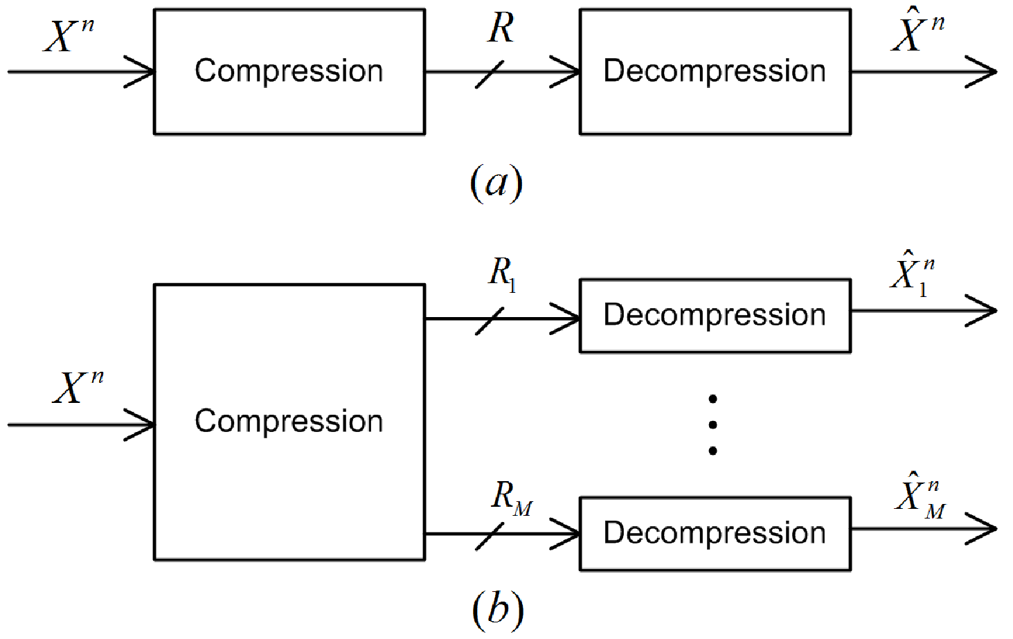
To fix the ideas and the notation, we first consider the conventional compression problem illustrated in Fig. 2-(a). The compression unit compresses a random sequence $X^{n}$ of $n$ independent and identically distributed (i.i.d.) samples with distribution $p(x)$ at a rate of $R$ bits per symbol. Specifically, the compressor selects a codeword $\hat{X}^{n}$ within a codebook $\mathcal{C}$ of size $2^{nR}$ and sends the corresponding index, of $nR$ bits, to the decompression unit. At the decompression unit, the sequence $\hat{X}^{n}\in\mathcal{C}$ indicated by the received index is recovered. Using the standard information-theoretic formulation, the compression strategy is specified by a conditional distribution $p(\hat{x}|x)$, which is referred to as the test channel (see, e.g., [12, Ch. 2]). For a given test channel, compression consists in selecting a sequence $\hat{X}^{n}\in\mathcal{C}$ that is jointly typical⁴⁴ 4 Two sequences $X^{n}$ and $Y^{n}$ are called jointly typical with respect to a distribution $p(x,y)$ if their joint empirical distribution (i.e., normalized histogram with step size $\Delta\rightarrow 0$) does not deviate much from $p(x,y)$ (see, e.g., [12, Ch. 2] for a formal definition). with the sequence $X^{n}$ with respect to the given joint distribution $p(x,\hat{x})=p(x)p(\hat{x}|x)$. Compression is hence successful if the encoder is able to find a jointly typical sequence $\hat{X}^{n}$ in the codebook $\mathcal{C}$. A classical result in information theory is that this happens with arbitrarily large probability as the block length $n$ grows large if the inequality

is satisfied [12, Ch. 3][30].

We now review the more general multivariate compression illustrated in Fig. 2-(b). Here, the sequence $X^{n}$ is compressed into $M$ indices with the goal of producing correlated compressed versions $\hat{X}_{1}^{n},\ldots,\hat{X}_{M}^{n}$. Each $i$th index indicates a codeword within a codebook $\mathcal{C}_{i}$ of size $2^{nR_{i}}$, and is sent to the $i$th decompression unit for $i\in\{1,\ldots,M\}$. Each $i$th decompression unit then recovers a sequence $\hat{X}_{i}^{n}\in\mathcal{C}_{i}$ corresponding to the received index. We emphasize that the choice of the codewords $\hat{X}_{1}^{n},\ldots,\hat{X}_{M}^{n}$ is done jointly at the compression unit. In particular, the specification of the compression strategy is given by a test channel $p(\hat{x}_{1},\ldots,\hat{x}_{M}|x)$. This implies that the compression unit wishes to find codewords $\hat{X}_{1}^{n},\ldots,\hat{X}_{M}^{n}$ that are jointly typical with the sequence $X^{n}$ with respect to the given joint distribution $p(x,\hat{x}_{1},\ldots,\hat{x}_{M})=p(x)p(\hat{x}_{1},\ldots,\hat{x}_{M}|x)$. The following lemma provides a sufficient condition for multivariate compression to be successful (we refer to [12, Lemma 8.2] for a more precise statement).

We observe that, for a given test channel $p(\hat{x}_{1},\ldots,\hat{x}_{M}|x)$, the inequalities (6) impose joint conditions on the rate of all codebooks. This is due to the requirement of finding codewords $\hat{X}_{1},\ldots,\hat{X}_{M}$ that are jointly correlated according to the given test channel $p(\hat{x}_{1},\ldots,\hat{x}_{M}|x)$. Also, note that the vector $X^{n}$ may be such that each $X_{i}$ is itself a vector and that the distortion requirements at each decompression unit prescribe that the decompression unit be interested in only a subset of entries in this vector. The connection between the multivariate set-up in Fig. 2-(b) and the system model under study in Fig. 1 will be detailed in the next section.

As mentioned in the previous section, the operation at the central encoder can be represented by the block diagram in Fig. 3. Specifically, after channel encoding, the encoded signals $\mathbf{s}=[\mathbf{s}_{1}^{\dagger},\ldots,\mathbf{s}_{N_{M}}^{\dagger}]^{\dagger}$ undergo precoding and compression, as detailed next.

1. Precoding: In order to allow for interference management both across the MSs and among the data streams for the same MS, the signals in vector $\mathbf{s}$ are linearly precoded via multiplication of a complex matrix $\mathbf{A}\in\mathbb{C}^{n_{B}\times n_{M}}$. The precoded data can be written as

where the matrix $\mathbf{A}$ can be factorized as

with $\mathbf{A}_{k}\in\mathbb{C}^{n_{B}\times n_{M,k}}$ denoting the precoding matrix corresponding to MS $k$. The precoded data $\tilde{\mathbf{x}}$ can be written as $\tilde{\mathbf{x}}=[\tilde{\mathbf{x}}_{1}^{\dagger},\ldots,\tilde{\mathbf{x}}_{N_{B}}^{\dagger}]^{\dagger}$, where the signal $\tilde{\mathbf{x}}_{i}$ is the $n_{B,i}\times 1$ precoded vector corresponding to the $i$th BS and given as

with the matrix $\mathbf{E}_{i}\in\mathbb{C}^{n_{B}\times n_{B,i}}$ having all zero elements except for the rows from $(\sum_{j=1}^{i-1}n_{B,j}+1)$ to $(\sum_{j=1}^{i}n_{B,j})$ which contain an $n_{B,i}\times n_{B,i}$ identity matrix. Note that non-linear precoding using DPC techniques can also be considered, as discussed in Remark 3 below.

2. Compression: Each precoded data stream $\tilde{\mathbf{x}}_{i}$ for $i\in\mathcal{N_{B}}$ must be compressed in order to allow the central encoder to deliver it to the $i$th BS through the backhaul link of capacity $C_{i}$ bits per c.u. Each $i$th BS then simply forwards the compressed signal $\mathbf{x}_{i}$ obtained from the central encoder. Note that this implies that the BSs need not be aware of the channel codebooks and of the precoding matrix $\mathbf{A}$ used by the central encoder. Instead, they must be informed about the quantization codebooks selected by the central encoder.

Using standard rate-distortion considerations, we adopt a Gaussian test channel to model the effect of compression on the backhaul link. In particular, we write the compressed signals $\mathbf{x}_{i}$ to be transmitted by BS $i$ as⁵⁵ 5 The test channel $\mathbf{x}_{i}=\mathbf{B}_{i}\tilde{\mathbf{x}}_{i}+\mathbf{q}_{i}$ is seemingly more general than (10), but this can be captured by adjusting the matrix $\mathbf{A}$ in (7).

where the compression noise $\mathbf{q}_{i}$ is modeled as a complex Gaussian vector distributed as $\mathcal{CN}(\mathbf{0},\mathbf{\Omega}_{i,i})$. Overall, the vector $\mathbf{x}=[\mathbf{x}_{1}^{\dagger},\ldots,\mathbf{x}_{N_{B}}^{\dagger}]^{\dagger}$ of compressed signals for all the BSs is given by

where the compression noise $\mathbf{q}=[\mathbf{q}_{1}^{\dagger},\ldots,\mathbf{q}_{N_{B}}^{\dagger}]^{\dagger}$ is modeled as a complex Gaussian vector distributed as $\mathbf{q}\sim\mathcal{CN}(\mathbf{0},\mathbf{\Omega})$. The compression covariance $\mathbf{\Omega}$ is given as

where the matrix $\mathbf{\Omega}_{i,j}$ is defined as $\mathbf{\Omega}_{i,j}=\mathbb{E}[\mathbf{q}_{i}\mathbf{q}_{j}^{\dagger}]$ and defines the correlation between the quantization noises of BS $i$ and BS $j$. Rate-distortion theory guarantees that compression codebooks can be found for any given covariance matrix $\mathbf{\Omega}\succeq\mathbf{0}$ under appropriate constraints imposed on the backhaul links’ capacities. This aspect will be further discussed in Sec. III-B.

With the described precoding and compression operations, the achievable rate (4) for MS $k$ is computed as

As explained above, due to the fact that the BSs are connected to the central encoder via finite-capacity backhaul links, the precoded signals $\tilde{\mathbf{x}}_{i}$ in (9) for $i\in\mathcal{N_{B}}$ are compressed before they are communicated to the BSs using the Gaussian test channels (10). In the conventional case in which the compression noise signals related to the different BSs are uncorrelated, i.e., $\mathbf{\Omega}_{i,j}=\mathbf{0}$ for all $i\neq j\in\mathcal{N_{B}}$ as in [21]-[24], the signal $\mathbf{x}_{i}$ to be emitted from BS $i$ can be reliably communicated from the central encoder to BS $i$ if the condition

is satisfied for $i\in\mathcal{N_{B}}$. This follows from standard rate-distortion theoretic arguments (see, e.g., [30] and Sec. III-A). We emphasize that (15) is valid under the assumption that each BS $i$ is informed about the quantization codebook used by the central encoder, as defined by the covariance matrix $\mathbf{\Omega}_{i,i}$.

In this paper, we instead propose to introduce correlation among the compression noise signals, i.e., to set $\mathbf{\Omega}_{i,j}\neq\mathbf{0}$ for $i\neq j$, in order to control the effect of the quantization noise at the MSs. As discussed in Sec. III, introducing correlated quantization noises calls for joint, and not independent, compression of the precoded signals of different BSs. As seen, the family of compression strategies that produce descriptions with correlated compression noises is often referred to as multivariate compression. By choosing the test channel according to (11) (see Sec. III-B), we can leverage Lemma 1 to obtain sufficient conditions for the signal $\mathbf{x}_{i}$ to be reliably delivered to BS $i$ for all $i\in\mathcal{N_{B}}$. In Lemma 2, we use $\mathbf{E}_{\mathcal{S}}$ to denote the matrix obtained by stacking the matrices $\mathbf{E}_{i}$ for $i\in\mathcal{S}$ horizontally.

Comparing (15) with (16) shows that the introduction of correlation among the quantization noises for different BSs leads to additional constraints on the backhaul link capacities.

Assuming the operation at the central encoder, BSs and MSs detailed above, we are interested in maximizing the weighted sum-rate $R_{\mathrm{sum}}=\sum_{k=1}^{N_{M}}w_{k}R_{k}$ subject to the backhaul constraints (16) over the precoding matrix $\mathbf{A}$ and the compression noise covariance $\mathbf{\Omega}$ for given weights $w_{k}\geq 0$, $k\in\mathcal{N_{M}}$. This problem is formulated as

The condition (17b) corresponds to the backhaul constraints due to multivariate compression as introduced in Lemma 2, and the condition (17c) imposes the transmit power constraints (1). It is noted that the problem (17) is not easy to solve due to the non-convexity of the objective function $\sum_{k=1}^{N_{M}}w_{k}f_{k}\left(\mathbf{A},\mathbf{\Omega}\right)$ in (17a) and the functions $g_{\mathcal{S}}\left(\mathbf{A},\mathbf{\Omega}\right)$ in (17b) with respect to $(\mathbf{A},\mathbf{\Omega})$. In Sec. V, we will propose an algorithm to tackle the solution of problem (17).

In order to obtain correlated quantization noises across BSs using multivariate compression, it is in principle necessary to perform joint compression of all the precoded signals $\tilde{\mathbf{x}}_{i}$ corresponding to all BSs $i$ for $i\in\mathcal{N_{B}}$ (see Sec. III-B). If the number of BSs is large, this may easily prove to be impractical. Here, we argue that, in practice, joint compression is not necessary and that the successive strategy based on MMSE estimation and per-BS compression illustrated in Fig. 4 is sufficient. The proposed approach works with a fixed permutation $\pi:\mathcal{N_{B}}\rightarrow\mathcal{N_{B}}$ of the BSs’ indices $\mathcal{N_{B}}$.

The central encoder first compresses the signal $\tilde{\mathbf{x}}_{\pi(1)}$ using the test channel (10), namely $\mathbf{x}_{\pi(1)}=\tilde{\mathbf{x}}_{\pi(1)}+\mathbf{q}_{\pi(1)}$, with $\mathbf{q}_{\pi(1)}\sim\mathcal{CN}(\mathbf{0},\mathbf{\Omega}_{\pi(1),\pi(1)})$, and sends the bit stream describing the compressed signal $\mathbf{x}_{\pi(1)}$ over the backhaul link to BS $\pi(1)$. Then, for any other $i\in\mathcal{N_{B}}$ with $i>1$, the central encoder obtains the compressed signal $\mathbf{x}_{\pi(i)}$ for BS $\pi(i)$ in a successive manner in the given order $\pi$ by performing the following steps:

(a) Estimation: The central encoder obtains the MMSE estimate $\mathbf{\hat{x}}_{\pi(i)}$ of $\mathbf{x}_{\pi(i)}$ given the signal $\tilde{\mathbf{x}}_{\pi(i)}$ and the previously obtained compressed signals $\mathbf{x}_{\pi(1)},\ldots,\mathbf{x}_{\pi(i-1)}$. This estimate is given by

where we defined the vector $\mathbf{u}_{\pi(i)}=[\mathbf{x}_{\pi(1)}^{\dagger},\ldots,\mathbf{x}_{\pi(i-1)}^{\dagger},\tilde{\mathbf{x}}_{\pi(i)}^{\dagger}]^{\dagger}$, and the correlation matrices $\mathbf{\Sigma}_{\mathbf{x}_{\pi(i)},\mathbf{u}_{\pi(i)}}$ and $\mathbf{\Sigma}_{\mathbf{u}_{\pi(i)}}$ are given as

and

with $\mathbf{\Omega}_{\mathcal{S},\mathcal{T}}=\mathbf{E}_{\mathcal{S}}^{\dagger}\mathbf{\Omega}\mathbf{E}_{\mathcal{T}}$ for subsets $\mathcal{S},\mathcal{T}\subseteq\mathcal{N_{B}}$ and the set $\mathcal{S}_{\pi,i}$ defined as $\mathcal{S}_{\pi,i}\triangleq\{\pi(1),\ldots,\pi(i)\}$.

(b) Compression: The central encoder compresses the MMSE estimate $\hat{\mathbf{x}}_{\pi(i)}$ to obtain $\mathbf{x}_{\pi(i)}$ using the test channel

where the quantization noise $\hat{\mathbf{q}}_{\pi(i)}$ is independent of the estimate $\hat{\mathbf{x}}_{\pi(i)}$ and distributed as $\hat{\mathbf{q}}_{\pi(i)}\sim\mathcal{CN}(\mathbf{0},\mathbf{\Sigma}_{\mathbf{x}_{\pi(i)}|\hat{\mathbf{x}}_{\pi(i)}})$ with

Note that the first equality in (23) follows from the fact that the MMSE estimate $\hat{\mathbf{x}}_{\pi(i)}$ is a sufficient statistic for the estimation of $\mathbf{x}_{\pi(i)}$ from $\mathbf{u}_{\pi(i)}$ (see, e.g., [36]). Moreover, the compression rate $I(\hat{\mathbf{x}}_{\pi(i)};\mathbf{x}_{\pi(i)})$ required by the test channel (22) is given by

To see why the structure in Fig. 4 described above realizes multivariate compression, we need the following lemma.

Lemma 3 shows that the region of backhaul capacities that guarantees correct delivery of the compressed signals (10) to the BSs, as identified in Lemma 2, is a type of polyhedron known as contrapolymatroid, as exemplified in Fig. 5. A specific feature of contrapolymatroid is that the corner points can be easily characterized as in (25). From standard rate-distortion theory arguments, the equality between (24) and (25) implies that the corner point $(C_{\pi(1)},\ldots,C_{\pi(N_{B})})$ can be obtained for any permutation $\pi$ by the successive estimation-compression strategy outlined above and illustrated in Fig. 4.

Overall, the discussion above shows that, for any correlation matrix $\mathbf{\Omega}$ in (12), multivariate compression is feasible by using the successive estimation-compression architecture in Fig. 4 if the backhaul capacities satisfy the corner point condition (25) for the given BS order $\pi$. Note that, in general, conditions (25) are more restrictive than (17b), which allows for any backhaul capacities in the contrapolymatroid. This is because the solution to the optimization problem (17) can be seen by contradiction to lie necessarily on the boundary of the region (17b) but possibly not on the corner points. Further discussion on this point can be found in Sec. V-B, where we observe that, in practice, this limitation is not critical.

As mentioned, the optimization (17) is a non-convex problem. To tackle this issue, we will now show how to obtain an efficient scheme that is able to achieve a stationary point of problem (17). To this end, we first make a change of variable by defining the variables $\mathbf{R}_{k}\triangleq\mathbf{A}_{k}\mathbf{A}_{k}^{\dagger}$ for $k\in\mathcal{N_{M}}$. Then, we define the functions $f_{k}\left(\{\mathbf{R}_{j}\}_{j=1}^{N_{M}},\mathbf{\Omega}\right)$ and $g_{\mathcal{S}}\left(\{\mathbf{R}_{k}\}_{k=1}^{N_{M}},\mathbf{\Omega}\right)$ with respect to the variables $\{\mathbf{R}_{k}\}_{k=1}^{N_{M}}$ which are obtained by substituting $\mathbf{R}_{k}=\mathbf{A}_{k}\mathbf{A}_{k}^{\dagger}$ into the functions $f_{k}\left(\mathbf{A},\mathbf{\Omega}\right)$ and $g_{\mathcal{S}}\left(\mathbf{A},\mathbf{\Omega}\right)$ in problem (17), respectively, and the transmit power constraint as $\mathrm{tr}\left(\sum_{k=1}^{N_{M}}\mathbf{E}_{i}^{\dagger}\mathbf{R}_{k}\mathbf{E}_{i}+\mathbf{\Omega}_{i,i}\right)\leq P_{i}$ for $i\in\mathcal{N_{B}}$. The so-obtained problem over the variables $\{\mathbf{R}_{k}\}_{k=1}^{N_{M}}$ and $\mathbf{\Omega}$ is still non-convex due to the second term in $f_{k}\left(\{\mathbf{R}_{j}\}_{j=1}^{N_{M}},\mathbf{\Omega}\right)$ and the first term in $g_{\mathcal{S}}\left(\{\mathbf{R}_{k}\}_{k=1}^{N_{M}},\mathbf{\Omega}\right)$, which are concave in the variables $\{\mathbf{R}_{k}\}_{k=1}^{N_{M}}$ and $\mathbf{\Omega}$. However, we observe that it falls into the class of difference-of-convex (DC) problems [38]. Among various algorithms having desirable properties for the solution of DC problems [38], we adopt the Majorization Minimization (MM) scheme [38], which solves a sequence of convex problems obtained by linearizing non-convex parts in the objective function $f_{k}\left(\{\mathbf{R}_{j}\}_{j=1}^{N_{M}},\mathbf{\Omega}\right)$ and the constraint function $g_{\mathcal{S}}\left(\{\mathbf{R}_{k}\}_{k=1}^{N_{M}},\mathbf{\Omega}\right)$. It is shown that the MM algorithm converges to a stationary point of the original non-convex problems (see, e.g., [34, Theorem 1], [38, Sec. 1.3.3] and [39, Theorem 3]). The proposed algorithm is summarized in Table Algorithm 1 where we define the functions $f_{k}^{\prime}(\{\mathbf{R}_{j}^{(t+1)}\}_{j=1}^{N_{M}},\mathbf{\Omega}^{(t+1)},\{\mathbf{R}_{j}^{(t)}\}_{j=1}^{N_{M}},\mathbf{\Omega}^{(t)})$ and $g_{\mathcal{S}}^{\prime}(\{\mathbf{R}_{j}^{(t+1)}\}_{j=1}^{N_{M}},\mathbf{\Omega}^{(t+1)},\{\mathbf{R}_{j}^{(t)}\}_{j=1}^{N_{M}},\mathbf{\Omega}^{(t)})$ as

and

with the function $\varphi(\mathbf{X},\mathbf{Y})$ given as

As we have discussed in Sec. IV, given the solution $(\mathbf{A},\mathbf{\Omega})$ obtained from the proposed algorithm, the central processor should generally perform joint compression in order to obtain the signals $\mathbf{x}_{i}$ to be transmitted by the BSs. However, as seen in Sec. IV-D, if the solution is such that the corner point conditions (25) are satisfied for a given permutation $\pi$ of the BSs’ indices, then the simpler successive estimation-compression structure of Fig. 4 can be leveraged instead. We recall, from Lemma 3, that in order to check whether the conditions (25) are satisfied for some order $\pi$, it is sufficient to observe which inequalities (17b) are satisfied with equality: If these inequalities correspond to the subsets $\mathcal{S}=\{\pi(1)\},\{\pi(1),\pi(2)\},\ldots,\{\pi(1),\ldots,\pi(N_{B})\}$ for a given permutation $\pi$, then the given solution corresponds to the corner point (25) with the given $\pi$. In our extensive numerical results, we have consistently found this condition to be verified. As a result, in practice, one can implement the compression strategy characterized by the calculated covariance $\mathbf{\Omega}$ by employing the implementation of Fig. 4 with the obtained ordering $\pi$.

For reference, it is useful to consider the weighted sum-rate maximization problem with independent quantization noises as in [21]-[24]. This is formulated as (17) with the additional constraints

Since the constraints (30) are affine, the MM algorithm in Table Algorithm 1 is still applicable by simply setting to zero matrices $\mathbf{\Omega}_{i,j}=\mathbf{0}$ for $i\neq j$ as per (30).

So far, we have assumed that the central encoder has information about the global channel matrices $\mathbf{H}_{k}$ for $k\in\mathcal{N_{M}}$. In this subsection, we discuss the robust design of the precoding matrix $\mathbf{A}$ and the compression covariance $\mathbf{\Omega}$ in the presence of uncertainty at the central encoder regarding the channel matrices $\mathbf{H}_{k}$ for $k\in\mathcal{N_{M}}$. Specifically, we focus on deterministic worst-case optimization under two different uncertainty models, namely singular value uncertainty [40] and ellipsoidal uncertainty models (see [41][42, Sec. 4.1] and references therein). While the singular value uncertainty model can be related via appropriate bounds to any normed uncertainty on the channel matrices, as discussed in [40, Sec. V], the ellipsoidal uncertainty model is more accurate when knowledge of the covariance matrix of the CSI error, due, e.g., to estimation, is available [42, Sec. 4.1]. In the following, we briefly discuss both models.

References

- [1] J. Andrews, "The seven ways HetNets are a paradigm shift," to appear in IEEE Comm. Mag., Mar. 2013.
- [2] Intel Cor., "Intel heterogeneous network solution brief," Solution brief, Intel Core Processor, Telecommunications Industry.
- [3] J. Segel and M. Weldon, "Lightradio portfolio-technical overview," Technology White Paper 1, Alcatel-Lucent.
- [4] S. Liu, J. Wu, C. H. Koh and V. K. N. Lau, "A 25 Gb/s(/km2) urban wireless network beyond IMT-advanced," IEEE Comm. Mag., pp. 122-129, Feb. 2011.
- [5] China Mobile, "C-RAN: the road towards green RAN," White Paper, ver. 2.5, China Mobile Research Institute, Oct. 2011.
- [6] T. Flanagan, "Creating cloud base stations with TI’s keystone multicore architecture," White Paper, Texas Inst., Oct. 2011.
- [7] Ericsson, "Heterogeneous networks," Ericsson White Paper, Feb. 2012.
- [8] P. Marsch, B. Raaf, A. Szufarska, P. Mogensen, H. Guan, M. Farber, S. Redana, K. Pedersen and T. Kolding, "Future mobile communication networks: challenges in the design and operation," IEEE Veh. Tech. Mag., vol. 7, no. 1, pp. 16-23, Mar. 2012.
- [9] V. Chandrasekhar, J. G. Andrews and A. Gatherer, "Femtocell networks: a survey," IEEE Comm. Mag., vol. 46, no. 9, pp. 59-67, Sep. 2008.
- [10] I. Maric, B. Bostjancic and A. Goldsmith, "Resource allocation for constrained backhaul in picocell networks," in Proc. ITA ’11, UCSD, Feb. 2011.
- [11] S. H. Lim, Y.-H. Kim, A. E. Gamal and S.-Y. Chung, "Noisy network coding," IEEE Trans. Inf. Theory, vol. 57, no. 5, pp. 3132-3152, May 2011.
- [12] A. E. Gamal and Y.-H. Kim, Network information theory, Cambridge University Press, 2011.
- [13] A. Sanderovich, O. Somekh, H. V. Poor and S. Shamai (Shitz), "Uplink macro diversity of limited backhaul cellular network," IEEE Trans. Inf. Theory, vol. 55, no. 8, pp. 3457-3478, Aug. 2009.
- [14] A. Sanderovich, S. Shamai (Shitz) and Y. Steinberg, "Distributed MIMO receiver - achievable rates and upper bounds," IEEE Trans. Inf. Theory, vol. 55, no. 10, pp. 4419-4438, Oct. 2009.
- [15] A. del Coso and S. Simoens, "Distributed compression for MIMO coordinated networks with a backhaul constraint," IEEE Trans. Wireless Comm., vol. 8, no. 9, pp. 4698-4709, Sep. 2009.
- [16] L. Zhou and W. Yu, "Uplink multicell processing with limited backhaul via successive interference cancellation," in Proc. IEEE Glob. Comm. Conf. (Globecom 2012), Anaheim, CA, Dec. 2012.
- [17] S.-H. Park, O. Simeone, O. Sahin and S. Shamai (Shitz), "Robust and efficient distributed compression for cloud radio access networks," IEEE Trans. Veh. Tech., vol. 62, no. 2, pp. 692-703, Feb. 2013.
- [18] M. Grieger, S. Boob and G. Fettweis, "Large scale field trial results on frequency domain compression for uplink joint detection," in Proc. IEEE Glob. Comm. Conf. (Globecom 2012), Anaheim, CA, Dec. 2012.
- [19] B. Nazer, A. Sanderovich, M. Gastpar and S. Shamai (Shitz), "Structured superposition for backhaul constrained cellular uplink," in Proc. IEEE Intern. Sym. Inf. Theory (ISIT 2009), Seoul, Korea, Jun. 2009.
- [20] S.-N. Hong and G. Caire, "Quantized compute and forward: a low-complexity architecture for distributed antenna systems," in Proc. IEEE Inf. Theory Workshop (ITW 2011), Paraty, Brazil, Oct. 2011.
- [21] O. Simeone, O. Somekh, H. V. Poor and S. Shamai (Shitz), "Downlink multicell processing with limited-backhaul capacity," EURASIP J. Adv. Sig. Proc., 2009.
- [22] P. Marsch and G. Fettweis, "On downlink network MIMO under a constrained backhaul and imperfect channel knowledge," in Proc. IEEE Glob. Comm. Conf. (Globecom 2009), Honolulu, Hawaii, Nov. 2009.
- [23] M. H. M. Costa, "Writing on dirty paper," IEEE Trans. Inf. Theory, vol. 29, no. 3, pp. 439-441, May 1983.
- [24] S.-N. Hong and G. Caire, "Reverse compute and forward: a low-complexity architecture for downlink distributed antenna systems," in Proc. IEEE Intern. Sym. Inf. Theory (ISIT 2012), Cambridge, MA, Jul. 2012.
- [25] B. L. Ng, J. S. Evans, S. V. Hanly and D. Aktas, "Distributed downlink beamforming with cooperative base stations," IEEE Trans. Inf. Theory, vol. 54, no. 12, pp. 5491-5499, Dec. 2008.
- [26] I. Sohn, S. H. Lee and J. G. Andrews, "Belief propagation for distributed downlink beamforming in cooperative MIMO cellular networks," IEEE Trans. Wireless Comm., vol. 10, no. 12, pp. 4140-4149, Dec. 2011.
- [27] R. Zakhour and D. Gesbert, "Optimized data sharing in multicell MIMO with finite backhaul capacity," IEEE Trans. Sig. Proc., vol. 59, no. 12, pp. 6102-6111, Dec. 2011.
- [28] O. Simeone, N. Levy, A. Sanderovich, O. Somekh, B. M. Zaidel, H. V. Poor and S. Shamai (Shitz), "Cooperative wireless cellular systems: an information-theoretic view," Foundations and Trends in Communications and Information Theory, vol. 8, nos. 1-2, pp. 1-177, 2012.
- [29] L. Zhang, R. Zhang, Y.-C. Liang, Y. Xin and H. V. Poor, "On Gaussian MIMO BC-MAC duality with multiple transmit covariance constraints," IEEE Trans. Inf. Theory, vol. 58, no. 4, pp. 2064-2078, Apr. 2012.
- [30] X. Zhang, J. Chen, S. B. Wicker and T. Berger, "Successive coding in multiuser information theory," IEEE Trans. Inf. Theory, vol. 53, no. 6, pp. 2246-2254, Jun. 2007.
- [31] R. Zhang, "Cooperative multi-cell block diagonalization with per-base-station power constraints," IEEE J. Sel. Areas Comm., vol. 28, no. 9, pp. 1435-1445, Dec. 2010.
- [32] M. Hong, R.-Y. Sun, H. Baligh and Z.-Q. Luo, "Joint base station clustering and beamformer design for partial coordinated transmission in heterogeneous networks," IEEE J. Sel. Areas Comm., vol. 31, no. 2, pp. 226-240, Feb. 2013.
- [33] C. T. K. Ng and H. Huang, "Linear precoding in cooperative MIMO cellular networks with limited coordination clusters," IEEE J. Sel. Areas Comm., vol. 28, no. 9, pp. 1446-1454, Dec. 2010.
- [34] M. Hong, Q. Li, Y.-F. Liu and Z.-Q. Luo, "Decomposition by successive convex approximation: a unifying approach for linear transceiver design in interfering heterogeneous networks," arXiv:1210.1507.
- [35] U. Erez and S. t. Brink, "A close-to-capacity dirty paper coding scheme," IEEE Trans. Inf. Theory, vol. 51, no. 10, pp. 3417-3432, Oct. 2005.
- [36] G. D. Forney, Jr., "Shannon meets Wiener II: On MMSE estimation in successive decoding schemes," arXiv:0409011v2.
- [37] D. N. C. Tse and S. V. Hanly, "Multiaccess fading channels-Part I: polymatroid structure, optimal resource allocation and throughput capacities," IEEE Trans. Inf. Theory, vol. 44, no. 7, pp. 2796-2815, Nov. 1998.
- [38] A. Beck and M. Teboulle, "Gradient-based algorithms with applications to signal recovery problems," in Convex Optimization in Signal Processing and Communications, Y. Eldar and D. Palomar, eds., pp. 42-88, Cambridge University Press. 2010.
- [39] G. Scutari, F. Facchinei, P. Song, D. P. Palomar and J.-S. Pang, "Decomposition by partial linearization: parallel optimization of multi-agent systems," arXiv:1302.0756v1.
- [40] S. Loyka and C. D. Charalambous, "On the compound capacity of a class of MIMO channels subject to normed uncertainty," IEEE Trans. Inf. Theory, vol. 58, no. 4, pp. 2048-2063, Apr. 2012.
- [41] C. Shen, T.-H. Chang, K.-Y. Wang, Z. Qiu and C.-Y. Chi, "Distributed robust multicell coordinated beamforming with imperfect CSI: an ADMM approach," IEEE Trans. Sig. Proc., vol. 60, no. 6, pp. 2988-3003, Jun. 2012.
- [42] E. Bjornson and E. Jorswieck, "Optimal resource allocation in coordinated multi-cell systems," Foundations and Trends in Communications and Information Theory, vol. 9, nos. 2-3, pp. 113-381, 2013.
- [43] S. Boyd and L. Vandenberghe, Convex optimization, Cambridge University Press, 2004.
- [44] D. Gesbert, S. Hanly, H. Huang, S. Shamai (Shitz), O. Simeone and W. Yu, "Multi-cell MIMO cooperative networks: a new look at interference," IEEE J. Sel. Areas Comm., vol. 28, no. 9, pp. 1380-1408, Dec. 2010.
- [45] H. Huh, H. C. Papadopoulos and G. Caire, "Multiuser MISO transmitter optimization for intercell interference mitigation," IEEE Trans. Sig. Proc., vol. 58, no. 8, pp. 4272-4285, Aug. 2010.
- [46] J. Lee and N. Jindal, "High SNR analysis for MIMO broadcast channels: dirty paper coding versus linear precoding," IEEE Trans. Inf. Theory, vol. 53, no. 12, pp. 4787-4792, Dec. 2007.