$XY\!Z$ Quantum Heisenberg Models with $p$-Orbital bosons

Introduction.– Powerful tools developed recently to unravel the physics of many-body quantum systems offer an exciting new platform for understanding quantum magnetism. It is now possible to engineer different systems in the lab that mimic the physics of theoretically challenging spin models [1], thereby performing “quantum simulations” [2]. Along these lines, systems of trapped ions and of polar molecules are promising candidates. Trapped ions, for example, have already been employed to simulate both small [3] and large [4] numbers of spins. In these setups, however, sustaining control over the parameters becomes very difficult as the system size increases. Furthermore, due to trapping potentials realizations are limited to chains with up to 25 spins. It is also very difficult to construct paradigmatic spin models with short range interactions using systems of trapped ions. Similar limitations appear when using polar molecules, where the effective spin interactions [5, 6] are obtained from the intrinsic dipole-dipole interactions. Due to the character of the dipolar interaction, these systems give rise to emergent models that are inherently long range and the resulting couplings usually feature spatial anisotropies.

Short range spin models can instead be realized with cold atoms in optical lattices [1]. A bosonic system in a tilted lattice has recently been used to simulate the phase transition in a 1D Ising model [7]. Fermionic atoms were employed to study dynamical properties of quantum magnetism for spin systems [8, 9]. This idea, first introduced in Ref. [10], has also been applied to other configurations, and simulation of different types of spin models have been proposed [11]. However, due to the character of the atomic $s$-wave scattering among the different Zeeman levels, such mappings usually yield effective spin models supporting continuous symmetries like the $X\!X\!Z$ model. But as the main goal of a quantum simulator is to realize systems that cannot be tackled via analytical and/or numerical approaches, it is important to explore alternative scenarios that yield low symmetry spin models with anisotropic couplings and external fields.

In this paper we propose such a scenario by demonstrating that bosonic atoms in the first excited band ($p$ band) of a two-dimensional (2D) optical lattice can realize the spin-$1/2$ $XY\!Z$ quantum Heisenberg model in an external field. Systems of cold atoms in excited bands feature an additional orbital degree of freedom [12] that gives rise to novel physical properties [13], which include supersolids [14] and other types of novel phases [15], unconventional condensation [16], and frustration [17]. Also a condensate with a complex order parameter was recently observed experimentally [4, 19]. The dynamics of bosons in the $p$ band include anisotropic tunneling and orbital changing interactions, where two atoms in one orbital state scatter into two atoms in a different orbital state. This is the key mechanism leading to the anisotropy of the effective spin model obtained here: These processes reduce the continuous $U(1)$ symmetry characteristic of the $X\!X\!Z$ model, which would effectively describe fermions in the $p$ band [20], into a set of discrete $Z_{2}$ symmetries characteristic of the $XY\!Z$ model. In addition, due to the anomalous $p$-band dispersions the couplings of the resulting spin model can favor for anti-ferromagnetic order even in the bosonic case.

We also demonstrate how further control of both the strength and sign of the couplings is obtained by external driving. This means that one can realize a whole class of anisotropic $XY\!Z$ models with ferromagnetic and/or anti-ferromagnetic correlations. To illustrate the rich physics that can be explored with this system we discuss the phase diagram of the $1D$ $XY\!Z$ chain in an external field. This case exhibits ferromagnetic as well as anti-ferromagnetic phases, a magnetized/polarized phase, a spin-flop and a floating phase [21]. Finite size effects relevant for the trapped case are examined via exact diagonalization. This reveals the appearance of a devil’s staircase manifested in the form of spin density waves. Finally, we discuss how to experimentally probe and manipulate the spin degrees of freedom.

$p$-orbital Bose system.– We consider bosonic atoms of mass $m$ in a 2D optical lattice of the form $V(\mathbf{r})=V_{x}\sin^{2}(k_{x}x)+V_{y}\sin^{2}(k_{y}y)$. Assuming that all atoms are in the first excited bands, the tight-binding Hamiltonian is

Here $\hat{a}_{i,\alpha}^{\dagger}$ creates a bosonic particle in the orbital $\alpha=p_{x},\,p_{y}$ at site $i$, $\hat{n}_{i,\alpha}=\hat{a}_{i,\alpha}^{\dagger}\hat{a}_{i,\alpha}$, and the sum is over nearest neighbors $i,j$. The tunneling matrix elements are given by $t^{\alpha}_{ij}=-\int d\mathbf{r}\,{w^{\alpha}_{i}}(\mathbf{r})^{*}\left[-\hbar^{2}\nabla^{2}/2m+V(\mathbf{r})\right]w^{\alpha}_{j}(\mathbf{r})$ where $w^{\alpha}_{i}(\mathbf{r})$ is the Wannier function of orbital $\alpha$ at site $i$. Note that $t^{\alpha}_{ij}$ is anisotropic. For instance, a boson in the $p_{x}$-orbital has a much larger tunneling rate in the $x$-direction than in the $y$-direction. The coupling constants are given by $U_{\alpha\alpha^{\prime}}=U_{0}\int d\mathbf{r}\,|w^{\alpha}_{i}(\mathbf{r})|^{2}|w^{\alpha^{\prime}}_{i}(\mathbf{r})|^{2}$, with $U_{0}>0$ the onsite interaction strength determined by the scattering length. The last term in (1) is the orbital changing term describing the flipping of a pair of atoms from the state $\alpha^{\prime}$ to the state $\alpha$. Note that this term is absent in the case of fermionic atoms.

Effective spin Hamiltonian.– We are interested in the physics of the Mott insulator phase with unit filling in the strongly repulsive limit $|t^{\alpha}_{ij}|^{2}\ll U_{\alpha\alpha^{\prime}}$. Projecting onto the Mott space of singly occupied sites with the operator $\hat{P}$, the Schrödinger equation becomes $\hat{H}_{\rm Mott}\hat{P}|\psi\rangle=E\hat{P}|\psi\rangle$ with $\hat{H}_{\rm Mott}=-\hat{P}\hat{H}(\hat{H}_{Q}-E)^{-1}\hat{H}\hat{P}$. Here $\hat{Q}=1-\hat{P}$ and $\hat{H}_{Q}=\hat{Q}\hat{H}\hat{Q}$ [22]. Since $E\sim t^{2}/U$, we can take $(\hat{H}_{Q}-E)^{-1}=\hat{H}_{Q}^{-1}$.

The space of doubly occupied states of a given site $j$ is three-dimensional and spanned by $|p_{x}p_{x}\rangle=2^{-1/2}\hat{a}_{jx}^{\dagger}\hat{a}_{jx}^{\dagger}|0\rangle$, $|p_{y}p_{y}\rangle=2^{-1/2}\hat{a}_{jy}^{\dagger}\hat{a}_{jy}^{\dagger}|0\rangle$, and $|p_{x}p_{y}\rangle=\hat{a}_{jx}^{\dagger}\hat{a}_{jy}^{\dagger}|0\rangle$. In this space, it is straightforward to find $\hat{H}_{Q}$ from (1), and subsequent inversion yields

with $U^{2}=U_{xx}U_{yy}-U_{xy}^{2}$. In particular, the off-diagonal terms in $\hat{H}_{Q}^{-1}$ derive from the orbital changing term. Using (2) we can now calculate all possible matrix elements of $\hat{H}_{Mott}$ in the Mott space,

where $\bar{x}=y$, and $\bar{y}=x$. By further employing the Schwinger angular momentum representation, $\hat{S}^{z}_{i}=\frac{1}{2}(\hat{a}^{\dagger}_{xi}\hat{a}_{xi}-\hat{a}^{\dagger}_{yi}\hat{a}_{yi})$, $\hat{S}^{+}_{i}=\hat{S}^{x}_{i}+i\hat{S}^{y}_{i}=\hat{a}^{\dagger}_{xi}\hat{a}_{yi}$ and $\hat{S}^{-}_{i}=\hat{S}^{x}_{i}-i\hat{S}^{y}_{i}=\hat{a}^{\dagger}_{yi}\hat{a}_{xi}$, together with the constraint $\hat{a}^{\dagger}_{xi}\hat{a}_{xi}+\hat{a}^{\dagger}_{yi}\hat{a}_{yi}=1$, we can (ignoring irrelevant constants) map (3) onto a spin-1/2 $XY\!Z$ model in an external field [23]

Here, $\langle i,j\rangle$ means summing over each nearest neighbor pair $i,j$ only once. The couplings are given by $J_{ij}=-2t^{x}_{ij}t^{y}_{ji}/U_{xy}$, $\gamma=-4U_{xy}^{2}/U^{2}$, and $\Delta_{ij}=-4(|t^{x}_{ij}|^{2}U_{yy}+|t^{y}_{ij}|^{2}U_{xx})/U^{2}+(|t^{x}_{ij}|^{2}+|t^{y}_{ij}|^{2})/U_{xy}$. The magnetic field is $h=4\sum_{\langle ij\rangle}(|t_{ij}^{y}|^{2}U_{xx}-|t_{ij}^{x}|^{2}U_{yy})/U^{2}+E_{p_{x}}-E_{p_{y}}$, where $E_{\alpha}$ is the onsite energy of the orbital $\alpha$.

Equation (4) is a main result of this paper. It demonstrates how $p$-orbital bosons in a 2D optical lattice can realize the $XY\!Z$ quantum spin-$1/2$ Heisenberg model. Several interesting facts should be noted. First, $t^{x}_{ij}t^{y}_{ji}<0$ due to the symmetry of the $p$-orbitals [12] and therefore $J_{ij}>0$. Furthermore, since $|\gamma|<1$ we have anti-ferromagnetic instead of the usual ferromagnetic couplings for bosons. Also, we obtain the $XY\!Z$ model when $\gamma\neq 0$. The presence of $\gamma$ can be traced to the orbital changing term in Eq. (1), which reduces the continuous $U(1)$ symmetry of $\hat{S}^{x}$ and $\hat{S}^{y}$ to a set of $Z_{2}$ symmetries. The $Z_{2}$ symmetries reflect the ‘parity’ conservation in the original bosonic picture which classifies the many-body states according to total even or odd number of atoms in the $p_{x}$ and $p_{y}$ orbitals. Since the orbital changing term is absent for fermions, the $XY\!Z$ model with anisotropic coupling is a peculiar feature of bosons in the $p$ band. We emphasize that the above derivation makes no assumptions regarding the geometry of the 2D lattice - i.e. it can be square, hexagonal etc.

1D $XY\!Z$ phase diagram.– To illustrate the rich physics of the $XY\!Z$ model, we now focus on the case of a 1D lattice where where quantum fluctuations are especially pronounced. Note that by increasing both the lattice amplitude and spacing in the $y$ direction keeping $V_{y}k_{y}^{2}\simeq V_{x}k_{x}^{2}$, one can exponentially suppress tunneling in the $y$ direction to obtain a 1D model, while the $p_{x}$ and $p_{y}$ orbitals are still quasi-degenerate [24]. In the 1D setting, we will drop the ”direction” subscript $ij$ on the coupling constants.

For 1D, the importance of the orbital changing term can be further illuminated, by employing the Jordan-Wigner transformation $\hat{S}_{i}^{-}=e^{i\pi\sum_{j=1}^{i-1}\hat{c}_{j}^{\dagger}\hat{c}_{j}}\hat{c}_{i}$ for fermionic operators $\hat{c}_{i}$. The result is the fermionic Hamiltonian

We see that $\gamma\neq 0$ leads to a pairing term that typically opens a gap in the energy spectrum. Incidentally the limit of $\Delta\rightarrow 0$ in Eq. (5) is a realization of the Kitaev chain [25].

The schematic phase diagram is illustrated in Fig. 1 (a). At zero field, the $XY\!Z$ model is integrable [26]. For large positive values of $\Delta/J$ the system is anti-ferromagnetic (AFM) in the $z$ direction. Small values of $\Delta/J$ are characterized by Néel ordering in the $y$ direction and the system is in the so-called spin-flop phase (SF). The $h=0$ line for large negative values of $\Delta/J$ is characterized by a ferromagnetic phase (FM) in the $z$ direction, and for all the cases, the limit of large external field displays a magnetized phase (PP), where the spins align along the orientation of the field in the $z$ direction. These three phases also characterize the phase diagram of the $XXZ$ model in a longitudinal field [27]. However, for non-zero anisotropy $\gamma$, a gapless floating phase (FP) emerges between the SF and the AFM phases which is characterized by power-law decay of the correlations [28, 21, 29]. The transition from the AFM to the FP is of the commensurate-incommensurate (C-IC) type whereas the transition between the FP and SF phases is of the Berezinsky-Kosterlitz-Thouless (BKT) type. For $\Delta<-(1+|\gamma|)$ there is a first order transition at $h=0$ between the two polarized phases. Finally, there is an Ising transition between the PP and the SF phases.

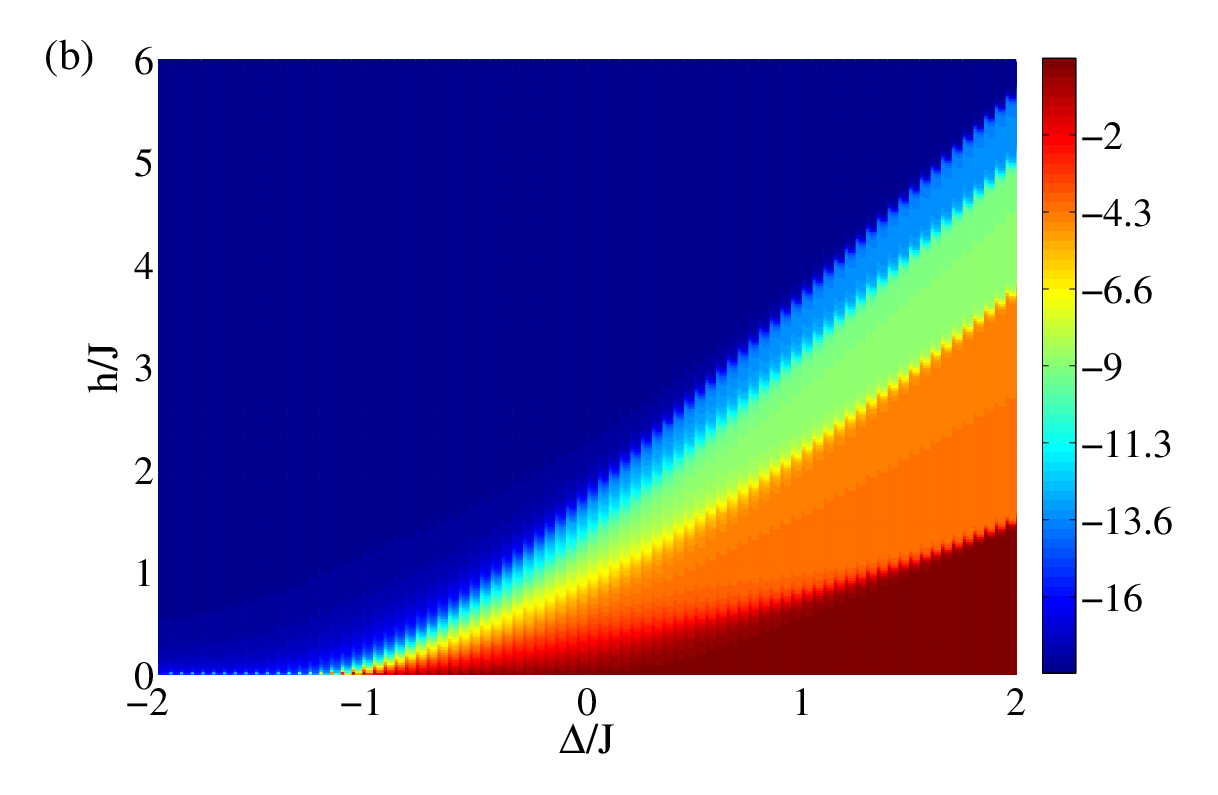
The experimental realization of the Heisenberg model will inevitably involve finite size effects due to the harmonic trapping potential. Within the local density approximation, the trap renormalizes the couplings so that they become spatially dependent [30], but this effect can be negligible if the orbitals are small compared to the length scale of the trap. In the regime of strong repulsion, the main effect of the trap is instead that it gives rise to “wedding cake” structures with Mott regions of integer filling. This effect was observed in the lowest band Bose-Hubbard model [1], and predicted theoretically to occur for anti-ferromagnetic systems [31]. To examine finite size effects, we have performed exact diagonalization in a chain with 18 spins with open boundary conditions. Figure 1 (b) displays the resulting finite size ’phase diagram’. The colors correspond to different values of the total magnetization $M=\sum_{i}\langle\hat{S}_{i}^{z}\rangle$ of the ground state. While the PP phase and the AMF phase are both clearly visible, the numerical results reveal a step like structure of the magnetization in between the two phases. We attribute these steps in $M$ to a devil’s staircase structure of spin-density-waves (SDW). As we see from Fig. 1 (b), it is only possible to give a numerical result for the PP-SF Ising transition. In particular, the C-IC and BKT transitions are overshadowed by the transitions between SDW. In the thermodynamic limit the staircase becomes complete and the changes in $M$ become smooth. One then recovers the phase diagram of Fig. 1 (a). These transitions, between different SDW, are more pronounced for moderate systems sizes. For a typical experimental system with $\sim$50 sites, for example, we estimate $\sim$15 different SDW between the AFM and PP phases.

Measurements and manipulations.– While time-of-flight measurements can reveal some of the phases [19], single-site addressing techniques [33] will be much more powerful when extracting correlation functions. To address single orbital states or even perform spin rotations, one may borrow techniques developed for trapped ions [3]. Making use of the symmetries of the $p_{x}$ and $p_{y}$ orbitals, stimulated Raman transitions can drive both sideband and carrier transitions for the chosen orbitals in the Lamb-Dicke regime. These transitions can be made so short that the system is essentially frozen during the operation. Driving sideband transitions in this way, spin rotations may be implemented. For example, a spin rotation around $x$ is achieved by driving the red-sidebands for both orbitals [23]. As a result, the two $p$ orbitals are coupled to the $s$ orbital in a $V$ configuration and in the large detuned case an adiabatic elimination of the $s$ band gives an effective coupling between the $p_{x}$ and $p_{y}$ orbitals [6]. This scheme, thus, realizes an effective spin Hamiltonian $\hat{H}_{x}^{(i)}=\frac{\Omega_{x}\Omega_{y}}{\Delta_{\mathrm{ps}}}\hat{S}_{i}^{x}$ with $\Omega_{\alpha}$ the effective Rabi frequencies and $\Delta_{\mathrm{ps}}$ the detuning. Alternatively, Stark-shifting one of the $p$ orbitals results in a rotation around $z$. Since the spin operators do not commute, any rotation can be realized from these two operations. Performing fluorescence on single orbital states by driving the carrier transition acts as measuring $\hat{S}_{i}^{z}$. This combined with the above mentioned rotations makes it possible to measure the spin at any site in any direction [23, 3].

Tuning of couplings.– For a square optical lattice, we have $U_{xx}=U_{yy}$. Moreover, in the harmonic approximation $U_{xy}=U_{xx}/3$, from which it follows that $\Delta<0$ and $\gamma=-1/2$. This gives ferromagnetic couplings for the $z$ component of neighboring spins, while the interactions between $x$ and between the $y$ components have anti-ferromagnetic couplings. We now show how the relative strength and sign of the different couplings can be controlled by squeezing one of the orbital states. Such squeezing can be accomplished by again driving the carrier transition of either of the two orbitals, dispersively with a spatially dependent field [23]. The shape of the drive can be chosen such that the resulting Stark shift is weaker in the center of the sites, resulting in a narrowing of the orbital. To be specific, assume that the ratio $\sigma$ of the harmonic length scales of the $p_{x}$ and $p_{y}$ orbitals in the $y$ direction is tuned. A straightforward calculation using harmonic oscillator functions yields $\alpha\equiv U_{xx}/U_{xy}=2^{-3/2}3(1+\sigma^{2})^{3/2}/\sigma$ and $\beta\equiv U_{yy}/U_{xy}=2^{-3/2}3(1+\sigma^{2})^{3/2}$. The coupling constants now depend on $\sigma$ as $\Delta/J=2t^{x}(t^{y})^{-1}\beta/(\alpha\beta-1)+2t^{y}(t^{x})^{-1}\alpha/(\alpha\beta-1)-(t^{x}/t^{y}+t^{y}/t^{x})/2$ and $\gamma=-4/(\alpha\beta-1)$. The inset in Fig. 3 displays the three coupling parameters as a function of $\sigma$ for $|t^{x}/t^{y}|=0.1$. We see that the relative size and even the sign of the couplings can be tuned by varying $\sigma$. In particular, while $\hat{S}_{y}$ always has AFM couplings, they can be made both FM or AFM for $\hat{S}_{x}$ and $\hat{S}_{z}$. In the main part of Fig. 3, we sketch the different accessible models as a function of $t^{y}/t^{x}$ and $\sigma$. This clearly demonstrates that one can realize a whole class of $XY\!Z$ spin chains by using this method.

Experimental realization.– In Ref. [4], the experimental realization of $p$-orbital bosons in an effective 1D optical lattice with a life-time of several milliseconds was reported. With an average number of approximately two atoms per site, the atoms could tunnel hundreds of times in the $p$ band before decaying. Since the main decay mechanism stems from atom collisions [32, 12], an increase of up to a factor of 5 in the lifetime is expected when there is only one atom per site [4]. Typical values of the couplings can be estimated from the overlap integrals of neighboring Wannier functions. Considering ⁸⁷Rb atoms, $\lambda_{lat}=843\,n$m and $V_{x}=30E_{R}$, $V_{y}=50E_{R}$ and $V_{z}=60E_{R}$, we obtain $J/E_{R}\sim 0.01$ and the characteristic tunneling time $\tau=\hbar/J\sim 5\,m$s. This corresponds to a few dozens of times smaller than the expected lifetimes [4], which should allow for experimental explorations of our results since relaxation typically occurs on a scale less than ten tuneling times [36]. In addition, as pointed out in [23], it is possible to increase the lifetimes even further with the use of external driving.

A major experimental challenge is to achieve a unit filling of the $p$ band. This could be achieved by having an excess number of atoms in the $p$ band and then adiabatically opening up the trap such that the unit filling is reached. A minority of sites will still be populated, however, by immobile $s$-orbital atoms. Since the interaction energy between $s$- and $p$-orbital atoms is higher than between two $p$-orbital atoms, processes involving $s$-orbital atoms will be suppressed. The presence of atoms in the $s$ band corresponds therefore to introducing static disorder in the system [23]. This may affect correlations [13], but the qualitative physics will remain unchanged for concentrations close to a unit filling. A more detailed study of this interesting effect is beyond the scope of the present work.

As a final remark we note that the spin correlations discussed here will emerge at temperatures $k_{B}T\lesssim J\sim t^{2}/U$ [10]. In addition, we estimate the required entropy [38] by equating the critical temperature $T_{c}$ to the gap between the ground and first excited states in the anti-ferromagnetic phase. Using the energy spectrum obtained from exact diagonalization, $S=(E-F)/T_{c}$ yields the entropy per particle $S/N=0.06k_{B}$. Experimentally one has in fact already achieved $S/N=0.05k_{B}$ [39], which indicates that our results are within experimental reach.

Conclusions.– We showed that the Mott regime of unit filling of bosonic atoms in the first excited bands of a 2D optical lattice realizes the spin-$1/2$ $XY\!Z$ quantum Heisenberg model. We then illustrated the rich physics of this model by examining the phase diagram of the 1D case. Finite size effects relevant to the trapped systems were discussed in detail. We proposed a method to control the strength and relative size of the spin couplings thereby demonstrating how one can realize a whole class of $XY\!Z$ models. We finally discussed experimental issues related to the realization of this model. We end by noting, that recent experiments reported a $\sim$99% loading fidelity of bosons into the $d$-band [11], which indeed opens possibilities to probe rich physics beyond spin-$1/2$ chains.

Acknowledgments.– We thank Alexander Altland, Alessandro De Martino, Henrik Johannesson, Stephen Powell, Eran Sela, and Tomasz Sowiński for helpful discussions. We acknowledge financial support from the Swedish research council (VR). GMB acknowledges financial support from NORDITA.

SUPPLEMENTARY MATERIAL

References

- [1] M. Lewenstein et al., Adv. Phys. 56, 243 (2007).
- [2] R. P. Feynman, Int. J. Theor. Phys. 21, 467 (1982).
- [3] A. Friedenauer et al., Nature Phys. 4, 757 (2008); K. Kim et al., Nature 465, 590 (2010); R. Islam et al., Nature Commun. 2, 377 (2011); R. Islam et al., arXiv:1210.0142; P. Richerme et al., arXiv:1303.6983.
- [4] J. W. Britton et al., Nature 484, 489 (2012).
- [5] A. Micheli, G. K. Brennen, and P. Zoller, Nature Phys. 2, 341 (2006).
- [6] B. Yan et al., arXiv:1305.5598.
- [7] J. Simon et al., Nature 472, 307 (2011).
- [8] T. Fukuhara et al., arXiv:1305.6559.
- [9] J. S. Krauser et al., Nature Phys. 8, 813 (2012); D. Greif et al., arXiv:1212.2634
- [10] L.-M. Duan, E. Demler, and M. D. Lukin, Phys. Rev. Lett. 91, 090402 (2003).
- [11] E. Altman, W. Hofstetter, E. Demler, M. Lukin, New J. Phys. 5 113, (2003), J. Radicć, A. DiCiolo, K. Sun, and V. Galitski, Phys. Rev. Lett. 109, 085303, (2012).
- [12] A. Isacsson and S. M. Girvin, Phys. Rev. A 72, 053604 (2005).
- [13] M. Lewenstein and W. V. Liu, Nature Phys. 7, 101 (2011).
- [14] V. W. Scarola and S. DasSarma, Phys. Rev. Lett. 95, 033003 (2005).
- [15] C. Xu and M. P. A. Fisher, Phys. Rev. B 75, 104428 (2007); J. Larson, A. Collin, and J.-P. Martikainen, Phys. Rev. A 79, 033603 (2009); A. Collin, J. Larson, and J. -P. Martikainen, Phys. Rev. A 81, 023605 (2010).
- [16] W. V. Liu and C. Wu, Phys. Rev. A 74, 013607 (2006); C. Wu, Mod. Phys. Lett. B 23, 1 (2009).
- [17] Z. Cai, Y. Wang and C. Wu, Phys. Rev. B 86, 060517(R) (2012).
- [18] T. Müller, S. Fölling, A. Widera, and I. Bloch, Phys. Rev. Lett. 99, 200405 (2007).
- [19] G. Wirth et al., Nature phys. 7, 147 (2011); P. Soltan-Panahi et al., Nature Phys. 8, 71 (2012).
- [20] C. Wu, Phys. Rev. Lett. 100, 200406 (2008); E. Zhao and W. V. Liu, Phys. Rev. Lett. 100, 160403 (2008).
- [21] E. Sela, A. Altland, and A. Rosch, Phys. Rev. B 84, 085114 (2011).
- [22] A. Auerbach, Interacting Electrons and Quantum Magnetism, (Springer, New York, 1998); F. Essler et al., The One-Dimensional Hubbard Model, (Cambridge University Press, Cambridge, 2005).
- [23] For more detailed calculations see the suplementary material.
- [24] X. Li, Z. Zhang, and W. V. Liu, Phys. Rev. Lett. 108, 175302 (2012).
- [25] A. Y. Kitaev Usp. Fiz. Nauk. (Suppl.) 171 10, 2001.
- [26] R. J. Baxter, Exactly Solvable Models in Statistical Mechanics (Academic Press, London, 1982)
- [27] H. Mikeska and H.-J. Kolezhuk, in Quantum Magnetism, U. Schollwöck, J. Richter, D. J. J. Farnell, R. F. Bishop (eds.), (Springer Verlag, Berlin, 2004).
- [28] P. Bak, Rep. Prog. Phys. 45 587 (1982).
- [29] In terms of bosonization (E. Miranda, Brazilian J. Phys. 33, 3 (2003)) and renormalization group arguments, the FP is characterized by irrelevant umklapp terms and accordingly described by the Luttinger liquid theory. Upon entering the XY phase these terms are no longer irrelevant and the phase becomes gapped. [21].
- [30] F. Pinheiro, J.-P. Martikainen, and J. Larson, Phys. Rev. A 85, 033638 (2012).
- [31] B. M. Andersen and G. M. Bruun, Phys. Rev. A 76, 041602 (2007).
- [32] J. Pietraszewicz et. al., arXiv:1303.5232v2 (2013).
- [33] W. S. Bakr et al., Nature 462, 74 (2009); J. F. Sherson et al., Nature 467, 68 (2010).
- [34] Chapter 5 and 6, Quantum Entanglement and Information Processing, Edited by D. Esteve, J.-M. Raimond, and J. Dalibard, (Eslevier, Amsterdam, 2004).
- [35] B. W. Shore, Manipulating Quantum Structures Using Laser Pulses, (Cambridge University Press, Cambridge, 2011).
- [36] M. Greiner et al, Nature, 415, 39-44 (2002).
- [37] C. A. Doty and D. S. Fisher, Phys. Rev. B 45, 2167 (1992).
- [38] L. Pollet et al., New J. Phys., 10 065001 (2008).
- [39] Markus Greiner, private communication.
- [40] Zhai, Yueyang, et. al., arXiv:1306.3313 (2013).
- [1] F. Essler, H. Frahm, F. Göhmann, A. Klumper and V. E. Korepin, The One-Dimensional Hubbard Model, Cambridge University Press, Cambridge, (2005).
- [2] C. Weitenberg et al., Nature 471, 319 (2011); T. Fukuhara et al., arXiv:1305.6559.
- [3] D. Leibfried et al., Rev. Mod. Phys. 75 281 (2003).
- [4] T. Müller et al., Phys. Rev. Lett. 99, 200405 (2007).
- [5] D. Wang et al., Phys. Rev. A 77, 053808 (2008).
- [6] B. W. Shore, Manipulating Quantum Structures Using Laser Pulses, (Cambridge University Press, Cambridge, 2011).
- [7] S. Haroche and J.-M. Raimond, Exploring the Quantum: Atoms, Cavities, and Photons, (Oxford University Press, Oxford, 2006).
- [8] M. Knap et al., arXiv:1307.0006.
- [9] J. Pietraszewicz et. al., arXiv:1303.5232v2 (2013).
- [10] A. Collin et al., Phys. Rev. A 81, 023605 (2010); T. Sowiński et al., arXiv:1304.6299.
- [11] Zhai, Yueyang et. al., arXiv:1306.3313 (2013).
- [12] G. Wirth et al., Nature phys. 7, 147 (2011); P. Soltan-Panahi et al., Nature Phys. 8, 71 (2012).
- [13] C. A. Doty and D. S. Fisher, Phys. Rev. B 45, 2167 (1992).