Perturbative solution to the SIS epidemic on networks

The single-city SIS model considers a large, well mixed, population, of size $N$, in some closed environment where death and birth are neglected. The population is divided into two compartments: susceptible, $S$; and infected, $I$; where $N=S+I=\textrm{constant}$. Both $S$ and $I$ are discrete variables. Susceptibles may become infected from contact with the infected at a rate $\beta$, and the infected compartment of the population will lose constituents at a rate $\gamma$. The mean-field dynamics of each state is then described by the set of equations:

where initial conditions are: $S(t=t_{0})=S_{0}>0$, and $I(t=t_{0})=I_{0}>0$. One immediately notes that $\partial_{t}\left[S(t)+I(t)\right]=0$, which then ensures that the total population, $N$, is constant for all time. It is noted that in the mean-field equations above, it is implicitly assumed that $S$ and $I$ are treated as continuous variables [2].

The solution to Eq. (2), and in turn Eq. (1), as $S(t)=N-I(t)$, is solved in various texts (for example see [2]), so for brevity, the solution is given ($t\geq t_{0}$):

where $\chi=\beta-\gamma$, and $I_{\infty}=\chi N/\beta$ is the stable or endemic state of the infected population; and $V=I_{\infty}/I_{0}-1$ [22]. With respect to Eq. (3), for an epidemic to take place (i.e. some finite fraction of the population remains infected in the long-time limit), we require the basic reproductive ratio: $R_{0}=\beta/\gamma$ to satisfy $R_{0}>1$ (which will be assumed henceforth).

To incorporate a spatial component to the model let us consider an arbitrary network of subpopulations.

We here further the result found in the previous section through incorporation of an implicit spatial component, by stratifying the large population into $M$ subpopulations (a realistic example is shown Fig. 1). Within each subpopulation (which may be regarded as a community, city, or country), the same assumptions stated in the canonical model still hold: the population is sufficiently large, and well mixed. One then allows for mobility between the nodes on the network, where the fraction of persons traveling from city $j$ to $i$ per unit time is given by the transport rate, $\omega_{i\leftarrow j}$.

Upon each node, an SIS virus is introduced, where the $i^{\textrm{th}}$ city has an infectivity rate of $\beta_{i}$, and recovery rate $\gamma_{i}$. The mean-field set of equations that then describe the dynamics are given by

where we have defined $\omega_{i\leftarrow i}=0$. A convenient parameter $\varepsilon(=1)$ is introduced here to keep track of the number of times the perturbation enters below (terms which are linear in $\varepsilon$ are linear in the travel rates etc) [24]. Summing Eq. (4) and Eq. (5), we find that $\partial_{t}N_{i}=0$, provided that the total influx and outflux for each node are equal, i.e.,

implying the total population $N_{i}$ of city $i$ is constant for all time. We will assume Eq. (6) to hold henceforth.

To begin the derivation of the perturbative solution, we first assume the influx and outflux of citizens from a given city is small (defined quantitatively later), from there we can define a perturbative solution in terms of the travel rates, namely

where $I^{(k)}_{i}(t)$ is the $k^{\textrm{th}}$ order contribution to the perturbative expansion at node $i$; i.e. $I_{i}^{(1)}$ contains only linear terms in the transport rates, whereas $I_{i}^{(2)}(t)$ contains only quadratics terms, and so on. In Eq. (6) $I_{i}^{(0)}(t)$ is given by Eq. (3), with replacements $\beta\rightarrow\beta_{i}$ and $\gamma\rightarrow\gamma_{i}$ (and therefore $\chi\rightarrow\chi_{i}$). Explicitly:

Similarly we can define the perturbative solution to the number of susceptibles in city $i$ as $S_{i}=\sum^{\infty}_{k=0}\varepsilon^{k}S^{(k)}_{i}$. Since $N_{i}=I_{i}^{(0)}+S_{i}^{(0)}$, it follows that $I_{i}^{(k)}=-S_{i}^{(k)}$ for $k\geq 1$. Using this fact and substituting Eq. (7) into Eq. (5) and equating factors of $\varepsilon^{k}$, we find for $k=0$, that $\partial_{t}I^{(0)}_{i}=\chi_{i}I^{(0)}_{i}-\frac{\beta_{i}}{N_{i}}\left[I_{i}^{(0)}\right]^{2},$ which is equivalent to Eq. (2), and whose solution is therefore given by Eq. (8). For $k\geq 1$ we obtain our formal perturbation equations

where we have set $\varepsilon=1$. Thus, we have formally converted the non-linear problem in Eq. (4) and Eq. (5) into a set of inhomogeneous, linear equations, Eq. (9), with time dependent coefficients. The time dependence of these coefficients in the left-hand-side enters only through the known quantity, $I_{i}^{(0)}(t)$, whereas the right-hand side depends recursively on the previous perturbation orders.

With regard to the initial condition of the system, the time $t_{0}$, viz. Eq. (8), need not be the true initial time, but rather some time at which $\vec{I}(t)(\equiv[I_{1}(t),I_{2}(t),\cdots,I_{M}(t)]^{T})$ is known. We will, in a subsequent section, utilize this freedom of choice in $t_{0}$ to improve upon the results in this section.

We proceed by expressing a formal solution to Eq. (9) through employment of the integrating factor method. Firstly, we define the so-called integrating factor: $\exp(B_{i}(t))$, where $B_{i}(t)=-\int^{t}_{t_{0}}\left[\chi_{i}-2\beta_{i}I_{i}^{(0)}(t^{\prime})/N_{i}\right]dt^{\prime}.$ Then the formal solution to the $k^{\textrm{th}}$-order perturbative term is $I^{(k)}_{i}(t)=\exp\left(-B_{i}(t)\right)\left[\int^{t}_{t_{0}}\exp\left(B_{i}(t^{\prime})\right)g_{i}^{(k-1)}(t^{\prime})dt^{\prime}+G_{i}^{(k)}\right],$ where, from the initial conditions: $I_{i}^{(k)}(t=t_{0})=0$, we have $G_{i}^{(k)}=0$. The function $g_{i}^{(k-1)}(t)$ is defined as

Interestingly, we are able to calculate $B_{i}(t)$ explicitly. Using Eq. (8), we can write $B_{i}(t)=-\chi_{i}(t-t_{0})+(2\beta_{i}I_{\infty,i})/(N_{i})\int^{t}_{t_{0}}(1+V_{i}e^{-\chi_{i}(t^{\prime}-t_{0})})^{-1}dt^{\prime}.$ We solve this to yield the solution $B_{i}(t)=\ln\left[e^{\chi_{i}(t-t_{0})}\left(\frac{1+V_{i}e^{-\chi_{i}(t-t_{0})}}{1+V_{i}}\right)^{2}\right].$ Using the solution for $B_{i}(t)$ and Eq. (10) and substituting this into the formal solution given, we explicitly obtain the $k^{\textrm{th}}$ order perturbation, namely

With this closed form expression, we are able to calculate any order perturbation we require, recursively. Namely, starting from the zeroth-order solution, Eq. (8), we can insert this into Eq. (10), the result of which is then input into Eq. (11) to find the first-order perturbation (shown explicitly in the following section). To find the next order, one uses the first-order result in place of the zeroth-order solution to, following the outlined algorithm, arrive at the second-order perturbation. This operation may be repeated until the desired number of orders are achieved. Then the orders are summed, viz. Eq. (7) (with $\varepsilon=1$), to gain the final solution to the infected population contained in city $i$.

Let us now calculate the first order perturbation term $k=1$. Then the function $g^{(0)}_{i}$, see Eq. (10), is explicitly: $g^{(0)}_{i}(t)=\sum_{j}\left(\omega_{i\leftarrow j}I^{(0)}_{j}-\omega_{j\leftarrow i}I^{(0)}_{i}\right),$ such that Eq. (11), using Eq. (8), becomes

where

The quantity $Q_{ij}$ may be expressed in terms of hypergeometric functions [25].

For the scope of this manuscript, let us analyze the case where we shall assume that all infection and recovery rate parameters are independent of the city, namely $\beta_{i}=\beta_{j}=\beta$ and $\gamma_{i}=\gamma_{j}=\gamma$. Explicitly evaluating Eq. (13), we find that

This leads to the explicit first-order perturbative contribution to Eq. (7),

where we have used Eq. (6). Eqs. (8) and (15), with $I_{i}(t)=I_{i}^{(0)}(t)+I_{i}^{(1)}(t)$ constitute the first-order solution to the SIS epidemic.

If instead of zero net nodal flux, Eq. (6), we instate the more restrictive clause of detailed balance [12], $\omega_{i\leftarrow j}N_{j}=\omega_{j\leftarrow i}N_{i}$, we have that $\omega_{i\leftarrow j}I_{\infty,j}=\omega_{j\leftarrow i}I_{\infty,i}$. Using this relation, we can write out the first order perturbation, Eq. (15), explicitly as

Summing this with the zeroth-order solution we reap the first-order perturbative approximation to the number of infected in city $i$ at time $t$:

where

and

The first-order approximation to $I_{i}(t)$, namely, Eq. (17), is valid when the perturbation due to mobility is “small”. To quantify explicitly the validity of Eq. (17) we introduce the approximate validity indicator:

For a given system, when $C_{i}(t_{0})\approx 0$ the zeroth-order solution is valid for $I_{i}(t)$; when $C_{i}(t_{0})\sim\mathcal{O}(1)$ the first-order solution is an accurate approximation to Eq. (5). For $C_{i}(t_{0})\gg 1$, Eq. (17) breaks down. It should be noted that $C_{i}(t_{0})$ may be valid for node $i$, but the corresponding indicator for some other node $j$ may not be. In this case, Eq. (17) would be reasonable still for $I_{i}(t)$, but not for $I_{j}(t)$, therefore caution is advised. In particular we point out that, besides the travel rate $\omega_{j\leftarrow i}$ (in units of $\beta$), also the fraction of initially infected for each node enters Eq. (18) in a non-trivial way. Eq. (18) requires that every neighboring node have a finite fraction of initially infected for Eq. (17) to be valid. This stems from the fact that if a node is initially uninfected, the transport of infected persons into that node, see Eq. (5), is no longer small (compared to the infectivity and recovery term), i.e. the base assumption of our perturbative approach is violated, therefore Eq. (17) breaks down. To remedy this initial condition restriction, we turn to linearization of the short-time dynamics in the next subsection.

We utilize the prerogative in the choice of $t_{0}$ in the previous section in order to generalize Eq. (17). We do this via approximating the short-time regime to allow for any initial state of the system, not only that all nodes be infected as required by the first-order perturbation result. We begin by neglecting the quadratic term $I_{i}^{2}N_{i}^{-1}$ in Eq. (5) (as it is generally small for short times compared to the linear term), thereby linearizing it to

This can be written as $\partial_{t}\vec{I}(t)\approx(\boldsymbol{\Omega}+\boldsymbol{\chi})\vec{I}(t)$, where $\Omega_{ij}=\omega_{i\leftarrow j}$ (for $i\neq j$), and $\Omega_{ii}=-\sum_{j}\omega_{j\leftarrow i}$. For the second matrix, $\boldsymbol{\chi}=\chi\boldsymbol{I}$ ($\boldsymbol{I}$ is the identity matrix). Through the Baker-Campbell-Hausdorff formula, and the commutativity of $\boldsymbol{\chi}$ and $\boldsymbol{\Omega}$, the general solution to this set of equations is

where $\vec{F}_{0}=\vec{I}(t=0)$ is the actual initial condition [26]. Note that $\vec{F}_{0}$ is different to the initial conditions used for the first-order perturbation result, i.e. $\vec{I}_{0}=\vec{I}(t=t_{0})$. In Eq. (20) the zeroth-order dynamics are captured via $\exp(\chi t)\vec{F}_{0}$, and the correction factor to the zeroth-order, captured in $\exp(\boldsymbol{\Omega}t)$, due to travel.

To find a limiting time for which Eq. (20) is valid, consider the following: we can recast Eq. (20) as

where the subscript $\alpha$ labels the eigenmode of the eigenvalue ($\lambda_{\alpha}$), to the corresponding left ($\vec{\ell}_{\alpha}$) and right ($\vec{r}_{\alpha}$) eigenvectors of $\boldsymbol{\Omega}$ [27]. We can approximate these exact linear dynamics by considering the contribution of only the leading eigenmode, $\alpha_{0}=0$ with $\lambda_{0}=0$ [28]. Then we have $\vec{\ell}_{0}=[1,1,\cdots,1]^{T}$, and $\vec{r}_{0}=N_{\textrm{tot}}^{-1}[N_{1},N_{2},\cdots,N_{M}]^{T}$, where $N_{\textrm{tot}}=\sum_{j=1}^{M}N_{j}$. So, per node, Eq. (21) simplifies to $I_{i}(t)\approx N_{\textrm{tot}}^{-1}N_{i}F_{0}^{\textrm{tot}}\exp(\chi t)$, where $F_{0}^{\textrm{tot}}=\sum_{j=1}^{M}F_{0,j}$. We wish to investigate where the linear approximation is valid, by comparing the linear and quadratic terms: $\beta/N_{i}I_{i}^{2}\ll\chi I_{i},$ or $I_{i}\ll N_{i}\chi\beta^{-1}\equiv I_{\infty,i}$. Using the $\alpha=0$ linear approximation for $I_{i}$ (as described above), we get that the linear approximation should be valid for $\exp(\chi t)N_{i}N_{\textrm{tot}}^{-1}F_{0}^{\textrm{tot}}\ll N_{i}\chi\beta^{-1}$ where the $N_{i}$ drops out, leaving us with $\exp(\chi t)\ll(\chi\beta^{-1})/(F_{0}^{\textrm{tot}}/N_{\textrm{tot}})$ which we recognize as the ratio between the asymptotic fraction of infecteds to the initial one. Thus we expect the linear approximation to break down as this limit saturates, i.e. at

A positive $t_{s}$ indicates that we need the initial linear stage, before switching to the non-linear dynamics in the perturbative approximation. A negative $t_{s}$, on the other hand, indicates that we can skip the linear step, and go directly to the nonlinear stage. Henceforth, $t_{s}$ will be referred to as the short-time limit.

If we are to "stitch" Eq. (20) to Eq. (17), we require that Eq. (17), be valid, i.e. $C_{i}(t_{0})\sim\mathcal{O}(1)$, where $t_{0}$ shall now be known as the stitch time. This criterion sets a soft lower bound to the use of Eq. (20). We establish a cut-off value of the validity indicator to be $C_{\textrm{cut},i}=C_{i}(t=t_{c})\sim\mathcal{O}(1)$. Then the time-frame for a suitable stitching is $t_{c}<t_{0}<t_{s}$. This stitched approximation allows us to model the full temporal dynamics of the network irrespective of the initial conditions.

To illustrate Eq. (20) and Eq. (21), we construct a simple system of two nodes, whose the eigenvalues are $\boldsymbol{\Omega}$ are $\{\lambda_{1},\lambda_{2}\}=\{0,-(\omega_{1\leftarrow 2}+\omega_{2\leftarrow 1})\}$ (see [28]), with the respective eigenvectors: $\vec{v}_{1}=[\omega_{1\leftarrow 2}\omega_{2\leftarrow 1}^{-1},1]^{T}$ and $\vec{v}_{2}=[-1,1]^{T}$. If we set the initial conditions, $\vec{I}(t=0)=[F_{0,1},0]^{T}$, then the nodal short-time evolution is: $I_{1}(t)=F_{0,1}\omega_{T}^{-1}[\omega_{2\leftarrow 1}\exp(\chi t)+\omega_{1\leftarrow 2}\exp([\chi-\omega_{T}]t)]$, $I_{2}(t)=F_{0,1}\omega_{2\leftarrow 1}\omega_{T}^{-1}[\exp(\chi t)-\exp([\chi-\omega_{T}]t)]$; where $\omega_{T}=\omega_{2\leftarrow 1}+\omega_{1\leftarrow 2}$.

In the event of an outbreak given the virus parameters mentioned above, we seek to understand how the country’s largest city, Auckland (Tāmaki Makaurau, subscript “Auck”), is affected and/or affects the remainder of NZ (subscript “rem”). We divide NZ into these two subpopulations (thereby assuming that each of these populations is well mixed). The documented transport rates between these two nodes are $\omega_{\textrm{rem}\leftarrow\textrm{Auck}}\approx 5.5\times 10^{-3}$ $\textrm{day}^{-1}$, and $\omega_{\textrm{Auck}\leftarrow\textrm{rem}}\approx 3.2\times 10^{-3}$ $\textrm{day}^{-1}$ [23], which are indeed small – as required by our perturbation assumption. We set the initial infected population to $F_{0,\textrm{Auck}}=100$, and $F_{0,\textrm{rem}}=0$, for Auckland and the remainder of NZ, respectively. Given these initial conditions and virus parameters, the short-time limit is $t_{s}\approx 200$ days. We use Eq. (20) to model the network until all nodes in the network are infected ($I_{i}(t)\geq 1,$ $\forall i$), and the validity indicator for Auckland, $C_{\textrm{Auck}}\leq 2$. At this time ($t_{0}\approx 108$ days) we use the state of the system as the initial condition for Eq. (17), and model the remaining infection dynamics for both nodes. We also compare our stitched first-order result to the stitched zeroth-order result (using Eq. (8) and Eq. (20)). This scenario of "no travel" can be likened to a situation of quarantine when all nodes have been found to be infected. It is also a measure of how effective the zeroth-order solution, Eq. (8), is at estimating the time-evolution of the epidemic. The stitched first-order and the stitched zeroth-order perturbation approximations are compared to the numerical solution, $\vec{I}_{\textrm{num}}(t)$ (calculated by the Runge-Kutta 4${}^{\textrm{th}}$ order algorithm) in Fig. 2.

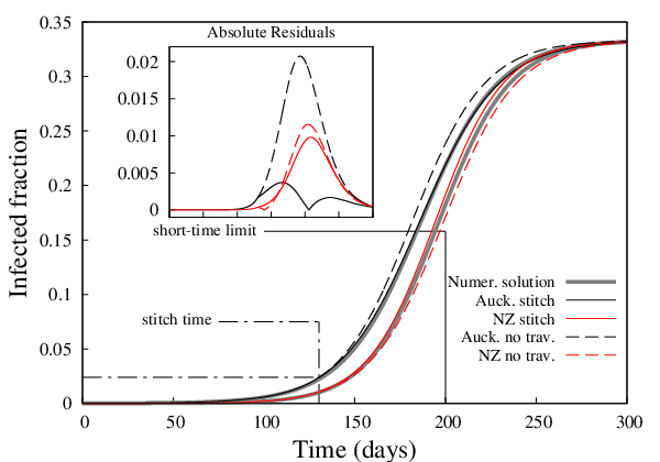
We note that, in Fig. 2, our analytical result conforms well to the numerical result, where the absolute residuals ($|\Delta_{j}(t)|$, see Appendix, Eq. (23)) between the first-order correction and the zeroth-order are given in the inset. The zeroth-order solution performs poorly at estimating the interim dynamics of the epidemic, especially underestimating the fraction of infected in Auckland.

To assess further the scope of our perturbation result, we reconstruct the system to include all available airports, giving a total of 23 nodes (see Fig. 1 and the Appendix). For this system we assume the same virus as before, with the same initially infected, whom have been introduced initially to the Auckland node (this again gives a short-time limit of $t_{s}\approx 200$ days). Again, we use Eq. (20) to simulate the short-time regime until all nodes are infected ($I_{i}(t)\geq 1$, $\forall i$), and the validity indicator for Auckland $C_{\textrm{Auck}}\leq 2$. At this time, $t_{0}\approx 127$ days, we use Eq. (17) to model the dynamics given the current state of the system. We plot these results for Auckland compared to the numerical solution and the stitched zeroth order approximation, Eqs. (8) and (20), in Fig. 3.

The choice of $t_{0}$ here favors a good validity indicator for Auckland. To understand the repercussion of this on other nodes in the network, alongside the infection dynamics of Auckland in Fig. 3, we have plotted the dynamics of Timaru (Te Tihi-o-Maru). Timaru has the highest validity at the stitch time, $C_{\textrm{Tim}}\approx 6.39$. This larger validity indicator makes for a worse approximation, as shown in Fig. (3), compared to Auckland with respect to the numerical solution. On the other hand, the stitched zeroth-order fares more poorly given this $t_{0}$. This highlights the subtle consequences in the choice of $t_{0}$.

References

- [1] W. O. Kermack and A. G. McKendrick, Proceedings of the Royal Society A: Mathematical, Physical and Engineering Sciences 115, 700 (1927)
- [2] H. W. Hethcote, in Three basic epidemiological models, Applied Mathematical Ecology, Vol. 18 (Springer Berlin Heidelberg, 1989) pp. 119–142
- [3] K. M. E. Turner, E. J. Adams, N. Gay, A. C. Ghani, C. Mercer, and W. J. Edmunds, Theoretical biology & medical modelling 3, 3 (2006)
- [4] J. Llibre and C. Valls, Journal of Mathematical Analysis and Applications 344, 574 (2008)
- [5] P. Das, Z. Mukandavire, C. Chiyaka, A. Sen, and D. Mukherjee, Differential Equations and Dynamical Systems 17, 393 (2010)
- [6] V. Méndez, D. Campos, and W. Horsthemke, Physical Review E 86 (2012)
- [7] D. T. Gillespie, Annual review of physical chemistry 58, 35 (Jan. 2007)
- [8] M. J. Keeling and J. V. Ross, Journal of the Royal Society, Interface / the Royal Society 5, 171 (Feb. 2008)
- [9] M. E. J. Newman, SIAM Review 45, 167 (2003)
- [10] O. Woolley-Meza, C. Thiemann, D. Grady, J. Lee, H. Seebens, B. Blasius, and D. Brockmann, The European Physical Journal B - Condensed Matter and Complex Systems, 1(2011)
- [11] J. P. Bagrow and Y.-R. Lin, PloS one 7, e37676 (2012)
- [12] D. Brockmann, in Reviews of Nonlinear Dynamics and Complexity, edited by H. G. Schuster (Wiley-VCH, 2009) pp. 1–24, ISBN 9783527408504
- [13] I. Hanski, Nature 396, 41 (1998)
- [14] B. Grenfell and J. Harwood, Trends in ecology & evolution 12 (1997)
- [15] H. Lund, L. Lizana, and I. Simonsen, Journal of Statistical Physics 151, 367 (2013)
- [16] V. Colizza and A. Vespignani, Physical Review Letters 99, 1 (2007)
- [17] R. Parshani, S. Carmi, and S. Havlin, Physical Review Letters 104, 258701 (Jun. 2010)
- [18] P. Van Mieghem and R. van de Bovenkamp, Physical Review Letters 110, 108701 (2013)
- [19] S. C. Ferreira, C. Castellano, and R. Pastor-Satorras, Physical Review E 86, 041125 (2012)
- [20] F. Arrigoni and A. Pugliese, Journal of mathematical biology 45, 419 (2002)
- [21] F. Ball, Mathematical Biosciences 156, 41 (1999)
- [22] In Ref. [2] the analytical solution of the SIS model with birth and death is provided. This solution can be used instead of Eq. (3) to yield an approximation to the temporal network dynamics following the derivation used here.
- [23] The air transport rates are calculated from the world-wide air traffic data provided by Ref. [32], taken the same year as the Subnational census data of NZ [29]. We have used the average number of available seats (from the total average flights) per day as the measure of the number of people commuting between two airport nodes in the NZ network. The travel weight is therefore the people leaving city as a fraction of . We have also removed all international connections to and from NZ airports.
- [24] J. J. Sakurai, Modern Quantum Mechanics (Revised Edition), 1st ed. (Addison Wesley, 1993) ISBN 0201539292
- [25] M. Abramowitz and I. A. Stegun, Handbook of Mathematical Functions with Formulas, Graphs, and Mathematical Tables, 9th ed. (Dover, 1972)
- [26] Using an eigenvalue approach allows us to numerically calculate at any desired (short) time without the need to introduce a time-step, as needed for instance in a Runge-Kutta approach.
- [27] For the case of different infectivity and recovery rates for the different cities, the matrix is replaced by a diagonal matrix with elements . For this case and do not commute in general, but the Baker-Campbell-Hausdorff formula still applies. This formula then requires us to evaluate a set of commutation relations in order to get an explicit expression for .
- [28] Using the Gershgorin circle theorem [35] for diagonally dominant square matrices, we find that the eigenvalues of in Eq. (20) have the following boundaries: , where defines the sum of rates away from node , , or the sum of the column of .
- [29] Statistics New Zealand, “Subnational Populations Estimates: At 30 June 2011,” http://www.stats.govt.nz/browse_for_stats/population/estimates_and_projections/SubnationalPopulationEstimates_HOTPJun11/Commentary.aspx (2011), [Online; accessed 4-April-2013]
- [30] The transport rates we use [32] satisfy the detailed balance condition, as required for the validity of Eq. (17).
- [31] We consider travel to and from the Chatham islands to be international travel and is therefore omitted.
- [32] OAG, “Air Traffic Data,” http://www.oag.com (2011), [Data retrieved: 03-Feb-2011]
- [33] L. Hufnagel, D. Brockmann, and T. Geisel, Proceedings of the National Academy of Sciences of the United States of America 101, 15124 (2004)
- [34] R. Levins, Bulletin of the Entomological Society of America 15, 237 (1969)
- [35] S. Gerschgorin, Bulletin de l’Académie des Sciences de l’URSS 6, 749 (1931)