Analysis of Spontaneous Mass Generation by Iterative Method
in the Nambu-Jona-Lasinio Model and Gauge Theories
Abstract
We propose a new iterative method to directly calculate the spontaneous mass generation due to the dynamical chiral symmetry breaking. We can conclude the physical mass definitely without recourse to any other consideration like the free energy comparison.
I Introduction
Owing to its outstanding feature, dynamical chiral symmetry breaking phenomena have been widely studied in various fields of elementary particle physics. The standard method to discuss the spontaneous mass generation is to formulate a coupled system of self-consistent equations and find its non-trivial solution. However, those equations are no more than the necessary condition and it is needed to examine solutions to select correct one by using another mean e.g. by referring to the free energy of each solution. Even if it is done, there are still unclear points whether the minimal free energy solution ensures the physically correct answer.
We adopt the Nambu-Jona-Lasinio (NJL) model[1] and give a new iteration method that directly sums up an infinite number of diagrams of the standard perturbation theory in the ladder approximation. Using this method, we demonstrate that the physically meaningful result is automatically obtained with the correct critical coupling constant. The NJL model has four-fermion interactions among the massless fermions with the chiral invariance. Here we added the bare mass to the Lagrangian to make the standard perturbation theory work well,
| (1) |
where is the number of fermion flavors. We consider leading contribution to the mass. Diagrammatically it is a sum of infinite diagrams called ‘tree’, where considering the fermion-antifermion pair as a single meson, the tree diagrams are defined by those without any meson loops, or in other words we regard a series of loops as a fat propagator.Usual method is to set up an equation satisfied by this infinite sum of diagrams. Above the critical coupling constant, there actually exists a non-trivial solution which does not vanish after zero bare mass limit. However, it is unclear that how the finite mass should come out of the infinite sum of the diagrams while each finite diagram must vanish at the zero bare mass limit. In this article we set up a method to directly sum up the infinite diagrams and show how the finite mass come out without any ambiguity[3].
II Iteration Method
First of all we classify diagrams in the tree using the node length of each diagram. Node length of a diagram is defined by the maximum number of loops in a continuous route towards the edge loop, or maximum number of nodes of fat propagator legs in the diagram. Fig. 1(a) shows the counting rule of node length and classification of diagrams. Here we define is a sum of diagrams whose node length is no greater than .


Then we write down the iteration to calculate by using as shown in Fig. 1(b). The transformation function is a one loop integral and we denote it by ,
| (2) |
Therefore the total sum of the tree diagrams is obtained by , infinitely many times of transformation of the same .
III Mass Generation
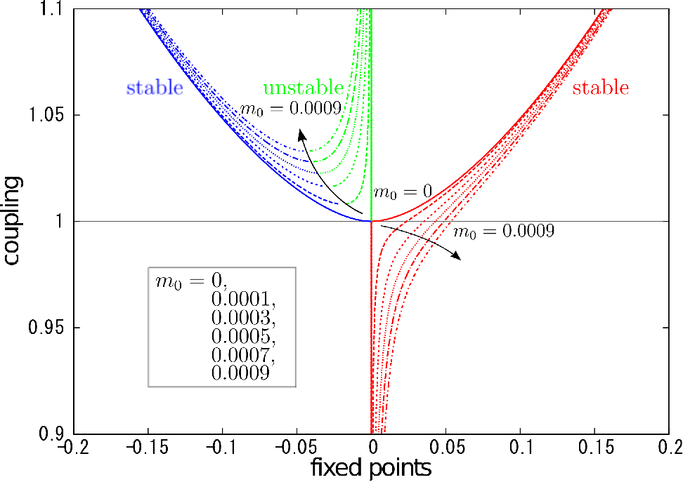
Iterative transformation here is best understood by a graphical method where the transformation function and a straight line of are drawn as shown in Fig. 2. Each iteration process can be drawn on this figure by a successive move of points. In any case the iterative transformation finally reaches a stable fixed point. Fixed points are crossing points between and , and position of fixed points are shown in Fig. 3.


In the weak coupling region, there is only one fixed point near the origin which is stable, and iteration from any starting point must reach it, as shown in Fig. 2(a). When the coupling constant becomes strong, there appear pair creation of fixed points, one is stable and the other is unstable. Then there are two stable fixed points each of which has its attractive region, ‘territory’. We must be careful about the initial starting point of iteration, that is, , which must be the bare mass by definition. In Fig. 3 we set a positive value for the bare mass, then the initial point is in the territory of the right-hand side stable fixed point, as seen in Fig. 2(b). Therefore for all region of the coupling constant, the physical result is controlled by the right most stable fixed point in Fig. 3. The critical coupling constant for the change of fixed point structure depends on the bare mass and it becomes unity in the vanishing bare mass limit.
Let’s see some features of mass generation with respect to the node length in Fig. 4. In the weak coupling case (a), the dynamical mass is generated rather quickly at low and becomes constant, which should be called the perturbative characteristics. By decreasing the bare mass the final mass goes to zero. In the strong coupling case (b), the generation of the dynamical mass depends strongly on the bare mass, and it is mainly generated at some narrow range of node length. Decreasing the bare mass, the region of mass generating node length becomes large, but the output mass is almost constant, which means the spontaneous mass generation. It is also seen that the shape of generation curves look the same form, just displacement in the node length space. These features are readily verified by the iterative nature of our calculation well seen in Fig. 2(b).


Finally we mention about gauge theories. We add all planar diagrams which are equivalent to the ladder Schwinger-Dyson equation[2]. To set up iterative method, we define ladder depth of each planar diagram which is the maximum number of gluon propagators towards the fermion propagator. We define mass function which contains all planar diagrams whose ladder depth is no greater than . Then we write down the iteration transformation as follows.
| (3) | |||||
| (4) |
where the mass function is a function of momentum squared . The functional is now an infinite dimensional map and there are infinite number of fixed point functions. Our analysis clarified that only one of fixed points is perfectly stable and reached by proper initial function [3].
References
- [1] Y. Nambu and G. Jona-Lasinio, Phys. Rev. 122, 345 (1961); 124, 246 (1961).
- [2] K-I. Aoki, M. Bando, T. Kugo, M.G. Mitchard and H. Nakatani, Prog. Theor. Phys. 84, 683 (1990).
- [3] K-I. Aoki, S. Onai and D. Sato in preparation.