Tracking the Tracker from its Passive Sonar ML-PDA EstimatesThanks: P. K. Willett was supported by ONR under contracts N00014-09-10613 and N10014-10-10412. Y. Bar-Shalom was supported by ARO under contract W911NF-10-10369 and ONR under contract N00014-10-1-0029.

Target motion analysis (TMA) with bearings-only measurements is a well-understood and extensively studied problem (see Fig. 1). It has been shown in the literature that as long as the platform is outmaneuvering the target, observability of the latter is assured and its motion can be inferred, even from very noisy measurements. Conversely, it is useful to understand whether, given the results of TMA estimation, it could be possible to identify, completely or at least partially, the trajectory of the observing platform.

More specifically, the problem arises when a “target-friendly” entity, as opposed to being cooperative with the platform, intercepts the results of the target estimation performed by the platform (see Fig. 2); the question is whether this entity can identify, partially or totally, the trajectory of the platform. The feasibility of this problem is of twofold interest: ($i$) it verifies the utility of intercepting communications (containing TMA-related information) between the platform and platform-cooperative entities, because this information would be useful; and ($ii$) it motivates, at the platform side, the need for secure and encrypted transmission of the TMA estimation results.

Seminal results on the continuous-time observability of the target motion, through a wideband passive sonar, were derived in [23, 13]. In fact, by successive differentiations of the measurement function, a necessary condition was derived and it was shown that a platform maneuver is a needed prerequisite to ensure observability of the target; however unobservable maneuvering-platform trajectories could exist (i.e. the platform may still take a trajectory wherefrom the target is unobservable). This analysis was rigorously extended, in the form of a necessary and sufficient condition, in [26, 12, 4, 18]; a comprehensive analysis of observability related to practical scenarios was also conducted in [18]. These results were also demonstrated in discrete-time in [14] via linear algebra; observability insights in different scenarios were presented, and also a stochastic observability (and estimability) analysis was performed. In [16] a theoretical connection between the invertibility of the Fisher information matrix (FIM) and target (local) observability was established. In [25] (and references therein) the optimal platform maneuver was designed, in the sense of the best estimation accuracy in terms of the FIM.

There are three common approaches to standard TMA (with or without Doppler measurements): maximum likelihood (ML), pseudolinear (PL) and instrumental variables (IV) estimation. Although the first approach is asymptotically efficient, it is complex and therefore suboptimal solutions are desirable. PL estimation has the advantage of being in closed form and of easy computation; however it can lead to severe bias even in favorable conditions [9]. Consequently IV estimation, yielding estimates with reduced bias, has seen recent attention [15, 10, 9, 11, 28].

Alternative bearings-only TMA scenarios have been studied recently in [3, 19, 8] and ML batch estimators have been proposed. More specifically, in [3] the problem of bearings-only TMA for conditionally-deterministic target motion and with operational constraints on the platform is tackled with Markov chain Monte Carlo methods. In [19] TMA of a maneuvering target and non-maneuvering platform is studied; observability is established and a batch estimator is proposed. The concept was later applied to the scenario of a circular constant-speed target and a non-maneuvering target in [8].

The estimators proposed in these references do not deal with the problem of false measurements (clutter) and less-than-unity probability of detection. The seminal work in [17] derived a ML estimate of target parameters for both wideband and narrowband passive sonars in the presence of false detections (clutter), based on probabilistic data association (ML-PDA); the performance of the estimator was evaluated in terms of the Cramér-Rao lower bound (CRLB). It was shown that the effect of the clutter on the performance through the CRLB was simply via a product with a less-than-unity scalar value, called the information reduction factor (IRF).

The ML-PDA was extended by incorporating amplitude information to enhance performance in the scenarios of “low-observable” (i.e. low Signal-to-Noise ratio) targets in [21]; improved accuracy and superior global convergence were demonstrated. In [7] ML-PDA was applied to the problem of low-observable target estimation using electro-optical sensors; also a sliding-window batch approach for ML-PDA estimation was derived, capable of dealing with temporary disappearance of targets and/or targets with velocities changing over time. ML-PDA was also successfully applied to active sonar tracking in [6], where also an efficient computation of the ML estimate, namely, directed subspace search (DSS), was derived. The use of ML-PDA for early track detection with a radar is discussed in [2].

The main contributions of the present paper are summarized as follows:

• •

  We study the “inverse” problem of identifying the platform trajectory, following a “two-leg” motion model, through its ML-PDA estimation results on a target; to the best of our knowledge, such a problem is addressed here for the first time.

• •

  We derive and study the objective function to be optimized for identifying the platform trajectory; it is shown that the optimization of this function depends on neither the IRF nor the measurement variance at the platform side; that is, the exact¹¹ 1 We will show however that for devising an efficient local-optimization algorithm a range of variability should be given; however the width of this range does not affect significantly the performance. information to identify the platform trajectory is unnecessary.

• •

  Also it is demonstrated that the platform trajectory is unobservable unless it keeps a constant speed during its two different legs.

• •

  We use an efficient and practical algorithm, based on a derivative-free local search, to solve the nonlinear problem associated with the identification task. The local optimization routine is initialized from geometric considerations and exploits the structure of the observed FIM.

The paper is organized as follows: In Sec. II we introduce the model for passive wideband-sonar localization and we give the background on the ML-PDA approach; in Sec. III we formulate the problem of inverse localization and we show some important identification properties; in Sec. IV we devise a procedure to compute a good initial estimate as input for the local optimization routines, while in Sec. V we show, by simulation, the performance of the proposed solution; some concluding remarks and future research are given in Sec. VI; proofs and derivations are confined to the Appendices.

Notation - Lower-case (resp. Upper-case) bold letters denote vectors (resp. matrices), with $a_{n}$ (resp. $A_{n,m}$) representing the $n$th (resp. the $(n,m)$th) element of the vector $\bm{a}$ (resp. matrix $\bm{A}$); upper-case calligraphic letters and braces denote finite sets, with $[a:b]$, $a\leq b$, representing the set $\{a,a+1,\ldots,b\}$; $\bm{I}_{N}$ denotes the $N\times N$ identity matrix, while $\mathrm{diag}\left(\bm{t}\right)$ is a diagonal matrix with diagonal equal to $\bm{t}$; $(\cdot)^{t}$,$\left\|\cdot\right\|_{2}$, $\left\|\cdot\right\|_{F}$ and $\left\langle\cdot\right\rangle$ denote transpose, $\ell_{2}$ norm, Frobenius norm and inner product operators, respectively; $\nabla_{\bm{t}}(\cdot)$ denotes the gradient operator w.r.t. the vector $\bm{t}$; $\bm{e}^{j}(\bm{A},i)$ denotes the unit eigenvector of a symmetric (and thus diagonalizable) matrix $\bm{A}$ (of size $[r\times r]$) corresponding to the eigenvalue $\lambda_{i}$, $i\in\mathcal{R}\triangleq\{1,\ldots r\}$, where $\lambda_{s}>\lambda_{s+1}$, $s\in\mathcal{R}\backslash\{r\}$, and $j\in\{-1,1\}$ denotes the sign ambiguity in the eigenvector formula; $\arctan_{2}(\bm{x})$, $\bm{x}\in\mathbb{R}^{2}$, denotes the four-quadrant inverse tangent with argument $\frac{x_{1}}{x_{2}}$; $P(\cdot)$ is used to denote probability mass functions (pmf) or probability density functions (pdf), while $P(\cdot|\cdot)$ is the corresponding conditional counterpart; $\mathcal{N}(\bm{\mu},\bm{\Sigma})$ denotes a real normal distribution with mean vector $\bm{\mu}$ and covariance matrix $\bm{\Sigma}$; finally the symbols $\rightarrow$, $\ni$, $\sim$, and $\perp$ mean “maps to”, “such that”, “distributed as” and “orthogonal”, respectively.

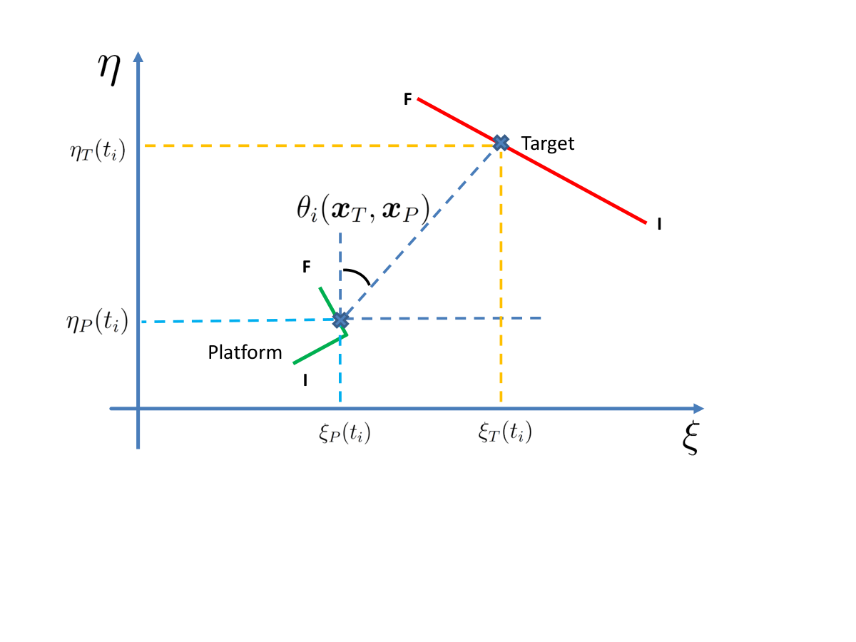
The system model is described graphically in Fig. 3. We assume that the target is observed by the platform at $n$ time samples, i.e. $t\in\mathcal{T}\triangleq\{t_{1},\ldots,t_{n}\}$; also we define the set of indices $\mathcal{I}\triangleq\{1,\ldots,n\}$. In the following we will explicitly list all the assumptions made, starting from the motion models of the platform and the target.

Assumption I: We assume that the target moves according to a constant velocity (CV) motion model [1]. For this reason we define $\bm{p}_{T}(t_{i})\triangleq\left[\begin{array}[]{cc}\xi_{T}(t_{i})&\eta_{T}(t_{i})\end{array}\right]^{t}$ and $\bm{v}_{T}\triangleq\left[\begin{array}[]{cc}\dot{\xi}_{T}&\dot{\eta}_{T}\end{array}\right]^{t}$ as the position at $t_{i}$ and the (constant) velocity 2-D vector of the target; $\xi$ and $\eta$ are used to denote the east and north directions. Given the CV assumption, $\{\bm{p}_{T}(t_{1}),\bm{p}_{T}(t_{n})\}$ uniquely define the state of the target at $t_{i}\in\mathcal{T}$. Therefore we stack them in $\bm{x}_{T}\triangleq\left[\begin{array}[]{cc}\bm{p}_{T}(t_{1})^{t}&\bm{p}_{T}(t_{n})^{t}\end{array}\right]^{t}$, which represents the true target state vector, unknown at the platform side. The target motion model has the explicit expression:

Assumption II: We assume a platform moving according to a “two-leg” motion model; this requirement not only ensures observability of the target from the platform point of view [23, 24], but also represents the easiest trajectory that can be followed by the platform. We denote $\bm{p}_{P}(t_{i})\triangleq\left[\begin{array}[]{cc}\xi_{P}(t_{i})&\eta_{P}(t_{i})\end{array}\right]^{t}$, $\bm{v}_{P,1}\triangleq\left[\begin{array}[]{cc}\dot{\xi}_{P,1}&\dot{\eta}_{P,1}\end{array}\right]^{t}$ and $\bm{v}_{P,2}\triangleq\left[\begin{array}[]{cc}\dot{\xi}_{P,2}&\dot{\eta}_{P,2}\end{array}\right]^{t}$, as the position at $t_{i}\in\mathcal{T}$, first-leg and second-leg velocity vectors; also we group $\bm{x}_{P}\triangleq\left[\begin{array}[]{ccc}\bm{p}_{P}(t_{1})^{t}&\bm{v}_{P,1}^{t}&\bm{v}_{P,2}^{t}\end{array}\right]^{t}$ into the platform state vector, representing the unknowns at the target-friendly side. Note that $\bm{x}_{P}$ does not uniquely define the platform trajectory, since the turning time $t_{k}$ is also needed.

Assumption III: Throughout this paper we will make the simplifying assumption that $t_{k}$ is known at the target-friendly side. In fact it is reasonable to assume that $t_{k}$ in practice will happen nearly the middle of the observation interval, i.e., $t_{k}\approx\frac{t_{n}-t_{1}}{2}$, in order to assure a good degree of observability²² 2 In fact, a turn at the beginning or the end of the observation interval would result in a platform trajectory similar to a single leg (CV model), thus leading to a nearly singular FIM.. This assumption will be relaxed in Sec. V, where a sensitivity analysis with respect to (w.r.t.) the timing-uncertainty on $t_{k}$ will be shown. Therefore, once $t_{k}$ is assumed to be known, the platform motion model is explicitly described as

Note that here the magnitudes of $\bm{v}_{P,1}$ and $\bm{v}_{P,2}$ are arbitrary. As shown later, unique identifiability of the platform trajectory (our goal) requires these magnitudes to be the same, i.e., the platform speed should be constant.

The statistical assumptions on the measurements are summarized as follows.

Assumption I: The bearing (true—originated from the target) measurement $\kappa_{i}$, collected by the platform at $t_{i}$, follows the model

where $\theta_{i}(\bm{x}_{T},\bm{x}_{P})$ denotes the noise-free bearing (we stress the dependence on both platform and target state vectors) and $n_{i}\sim\mathcal{N}(0,\sigma_{\theta}^{2})$. For notational convenience we also define here the range $r_{i}(\bm{x}_{T},\bm{x}_{P})$ as

Assumption II: We assume, as in realistic environments, that a passive sonar at $t_{i}\in\mathcal{T}$ collects a set of measurements $\bm{z}(i)$, due to clutter and non-perfect detection. More specifically, we have

where $m_{i}$ denotes the number of collected measurements at $t_{i}\in\mathcal{T}$. The statistical assumptions over the set in Eq. (8) are: ($i$) the true measurement $\kappa_{i}$ can be detected at most only once, with probability $P_{D}$; ($ii$) the number of false measurements at $t_{i}\in\mathcal{T}$ follows a known probability mass function $\mu_{F}(\cdot)$, given by a Poisson law with known expected number of false alarms per unit of volume $\lambda$; therefore the false measurements are distributed uniformly and independently in the surveillance region (in the bearing space).

Assumption III: We assume conditional mutual independence among the sets of measurements, that is $P(\bm{z}(i_{1}),\bm{z}(i_{2})|\bm{x}_{T},\bm{x}_{P})=P(\bm{z}(i_{1})|\bm{x}_{T},\bm{x}_{P})P(\bm{z}(i_{2})|\bm{x}_{T},\bm{x}_{P})$, $\forall i_{1}\neq i_{2}$.

Under these assumptions and denoting $\bm{\breve{x}}_{T}$ (resp. $\bm{\breve{x}}_{P}$) as the true target (resp. platform) state vector, the ML-PDA estimate $\bm{\hat{x}}_{T}$ is obtained as

where the likelihood of $\bm{x}_{T}$ is given by:

Note that $\bm{\breve{x}}_{P}$ is assumed known at the platform side. It was shown numerically in [17] that the covariance matrix of the ML-PDA estimator essentially attains the CRLB and therefore it can be regarded as an efficient estimator. For this reason, the covariance matrix is approximated by the inverse of the FIM given by

where $\alpha_{\theta}$ is defined as³³ 3 Note that $\alpha_{\theta}$ should not be confused with $\alpha_{i}=\frac{t_{i}-t_{1}}{t_{n}-t_{1}}$ defined in Eq. (4).

with $q_{2}$ representing the IRF [17, 2]. Note that

where $v_{g}$ and $g$ denote the volume of the validation region and the gating threshold, respectively. It can be shown, after some manipulations, that $\bm{\nabla}_{\bm{x}_{T}}(\theta_{i}(\bm{x}_{T},\bm{x}_{P}))$ has the explicit expression

The FIM at the platform side is necessarily evaluated as $\bm{J}^{obs}\triangleq\bm{J}(\bm{\breve{x}}_{P},\bm{\hat{x}}_{T},\breve{\alpha}_{\theta})$, where $\breve{\alpha}_{\theta}$ denotes the true $\alpha_{\theta}$, known at the platform side. Given the results of the estimation process at the platform side, that is $\{\bm{\hat{x}}_{T},\bm{J}^{obs}\}$, our task can be summarized as follows.

We wish to identify the platform state, represented by $\bm{x}_{P}$, by observing only the estimation results of the ML-PDA, that is $\{\bm{\hat{x}}_{T},\bm{J}^{obs}\}$. It is worth remarking that the unknowns of this deterministic problem are represented by $\{\bm{\breve{x}}_{P},\breve{\alpha}_{\theta}\}$. In fact, even if $\breve{\alpha}_{\theta}$ does not contribute to specifying the platform trajectory, it has to be identified to solve this task.

The first important remark is that the identification problem is a function only of $\bm{\hat{x}}_{T}$ rather than the true trajectory $\bm{\breve{x}}_{T}$. This has an important consequence: the identification of the platform trajectory does not depend on the true target trajectory $\bm{\breve{x}}_{T}$; however we will show that due to the sensitivity w.r.t. the true platform parameters, a larger FIM matrix will lead to an easier identification in terms of local optimization routines.

It can be easily shown that $\{\bm{\breve{p}}_{P}(t_{1}),\bm{\breve{p}}_{P}(t_{n})\}$ can be expressed in the form:

In order to obtain good estimates $\{\bm{\hat{p}}_{P}(t_{1}),\bm{\hat{p}}_{P}(t_{n})\}$ we need to find good approximations $\{\hat{r}_{1},\hat{r}_{n}\}$ and $\{\hat{\bm{i}}_{1},\bm{\hat{i}}_{n}\}$. These issues can be tackled separately.

As pointed out previously, Eqs. (46) and (47) define two pairs $\{\bm{\hat{p}}_{P}^{g}(t_{1}),\bm{\hat{p}}_{P}^{g}(t_{n})\}$, $g\in\{1,2\}$. Hence for each $\{\bm{\hat{p}}_{P}^{g}(t_{1}),\bm{\hat{p}}_{P}^{g}(t_{n})\}$ a corresponding $\bm{\hat{p}}_{P}^{g}(t_{k})$ needs to be computed. In this case it can be shown that $\bm{\hat{p}}_{P}^{g}(t_{k})$ cannot be chosen only relying on the geometric properties of the FIM, as opposed to $\bm{\hat{p}}_{P}(t_{1})$ and $\bm{\hat{p}}_{P}(t_{n})$. Rather, a $\pm\frac{\pi}{2}$ platform turn initial assumption is made and the turn-sign ambiguity is solved exploiting the coarse information in the FIM. By defining $t_{m}\triangleq\arg\min_{t_{i}\in\mathcal{T}}\left\|t_{i}-\frac{t_{n}-t_{1}}{2}\right\|_{2}$, such a vector is obtained as (we drop the superscript $g$)

where $\bm{\rho}_{\ell}(t_{m})$ is the position vector at $t_{m}$ of the two-leg trajectory described by $\{\hat{\bm{p}}_{P}(t_{1}),\bm{\rho}_{\ell}(t_{k}),\hat{\bm{p}}_{P}(t_{n})\}$, and $\tilde{\bm{p}}{}_{P}(t_{m})$ is given by

The complete derivation of the selection of $\bm{\hat{p}}_{p}^{g}(t_{k})$ is given in Appendix G.

The presented method computes $\hat{\bm{p}}_{P}^{g}=\left[\begin{array}[]{ccc}\hat{\bm{p}}_{P}^{g}(t_{1})^{t}&\hat{\bm{p}}_{P}^{g}(t_{k})^{t}&\hat{\bm{p}}_{P}^{g}(t_{n})^{t}\end{array}\right]^{t}$, $g\in\{1,2\}$, under the assumption that $\breve{\alpha}_{\theta}$ is known at the target-friendly side. However, since $\breve{\alpha}_{\theta}$ is known exactly only at the platform side, we will replace $\breve{\alpha}_{\theta}$ with the variable $\alpha_{\theta}$ in Eq. (37), thus leading to $\hat{\bm{p}}_{P}^{g}=\hat{\bm{p}}_{P}^{g}(\alpha_{\theta})$, i.e., a continuum of initial guesses. Therefore, in order to obtain a (small) finite set of initial guesses we apply the following steps:

1. 1.

   define a uniform grid of $N_{\theta}$ values on $\alpha_{\theta}$, constrained in the interval $[\alpha_{\theta,\min},\alpha_{\theta,\max}]$⁷⁷ 7 The values $\{\alpha_{\theta,\min},\alpha_{\theta,\max}\}$ are obtained automatically, once a reasonable range is given for parameters concurring with the definition of $\alpha_{\theta}$ (e.g. $\sigma_{\theta}$); an example will be given in Section V. and, after denoting the $m$-th value as $\alpha_{\theta}[m]=\alpha_{\theta,\min}+\frac{m-1}{N_{\theta}-1}(\alpha_{\theta,\max}-\alpha_{\theta,\min})$, $m\in\mathcal{S}_{\theta}\triangleq\{1,\ldots,N_{\theta}\}$, we compute $\hat{\bm{p}}_{P}^{g}(\alpha_{\theta}[m])$, $g\in\{1,2\}$, $m\in\mathcal{S}_{\theta}$;

2. 2.

   split up the set $\hat{\bm{p}}_{P}^{g}(\alpha_{\theta}[m])$, $m\in\mathcal{S}_{\theta},g\in\{-1,1\}$ into three subsets, corresponding to zones ($a$), ($b$) and ($c$), defined as follows⁸⁸ 8 Note that the definition of the zones is arbitrary.: ($i$) we split $\hat{\bm{p}}_{P}^{g}(\alpha_{\theta}[m])$ into two sets $\hat{\bm{p}}_{P}^{g=1}(\alpha_{\theta}[m])$ and $\hat{\bm{p}}_{P}^{g=-1}(\alpha_{\theta}[m])$; $(ii)$ by defining $\Gamma_{m,g}\triangleq\arctan_{2}\left(\hat{\bm{p}}_{P}^{g}(t_{n},\alpha_{\theta}[m])-\hat{\bm{p}}_{P}^{g}(t_{1},\alpha_{\theta}[m])\right)$ we seek for $\{m^{*},g^{*}\}\ni\mathrm{sign}(\Gamma_{m^{*},g^{*}})\neq\mathrm{sign}(\Gamma_{(m^{*}+1),g^{*}})$; ($iii$) we split the set corresponding to $g^{*}$ as $\hat{\bm{p}}_{P}^{g^{*}}(\alpha_{\theta}[1:m^{*}])$ and $\hat{\bm{p}}_{P}^{g^{*}}(\alpha_{\theta}[(m^{*}+1):N_{\theta}])$;

3. 3.

   choose, from each defined subset, the guess corresponding to the maximum of Eq. (32), and denote the obtained triple as $\{\hat{\bm{p}}_{P}^{A},\hat{\bm{p}}_{P}^{B},\hat{\bm{p}}_{P}^{C}\}$, which is fed (possibly in parallel) to a local optimization routine.

References

- [1] Y. Bar-Shalom, T. Kirubarajan, and X. R. Li, Estimation with Applications to Tracking and Navigation. New York, NY, USA: John Wiley & Sons, Inc., 2001.
- [2] Y. Bar-Shalom, P. K. Willett, and X. Tian, Tracking and Data Fusion: A Handbook of Algorithms. YBS publishing, 2011.
- [3] F. Bavencoff, J. M. Vanpeperstraete, and J.-P. Le Cadre, “Constrained bearings-only target motion analysis via Markov chain Monte Carlo methods,” IEEE Trans. Aerosp. Electron. Syst., vol. 42, no. 4, pp. 1240–1263, Oct. 2006.
- [4] K. Becker, “Simple linear theory approach to TMA observability,” IEEE Trans. Aerosp. Electron. Syst., vol. 29, no. 2, pp. 575–578, Apr. 1993.
- [5] D. S. Bernstein, Matrix Mathematics: Theory, Facts, and Formulas with Application to Linear Systems Theory. Princeton University Press, Feb. 2005.
- [6] W. R. Blanding, P. K. Willett, Y. Bar-Shalom, and R. Lynch, “Directed subspace search ML-PDA with application to active sonar tracking,” IEEE Trans. Aerosp. Electron. Syst., vol. 44, no. 1, pp. 201–216, Jan. 2008.
- [7] M. R. Chummun, Y. Bar-Shalom, and T. Kirubarajan, “Adaptive early-detection ML-PDA estimator for LO targets with EO sensors,” IEEE Trans. Aerosp. Electron. Syst., vol. 38, no. 2, pp. 694–707, Apr. 2002.
- [8] J. Clavard, D. Pillon, A.-C. Pignol, and C. Jauffret, “Bearings-only target motion analysis of a source in a circular constant speed motion from a non-maneuvering platform,” in Proceedings of the 14th International Conference on Information Fusion (FUSION), Jul. 2011, pp. 1–8.
- [9] K. Doğançay, “On the bias of linear least squares algorithms for passive target localization,” Signal Processing, vol. 84, no. 3, pp. 475–486, Mar. 2004.
- [10] ——, “Passive emitter localization using weighted instrumental variables,” Signal Processing, vol. 84, no. 3, pp. 487–497, 2004.
- [11] ——, “On the efficiency of a bearings-only instrumental variable estimator for target motion analysis,” Signal Processing, vol. 85, no. 3, pp. 481–490, Mar. 2005.
- [12] E. Fogel and M. Gavis, “Nth-order dynamics target observability from angle measurements,” IEEE Trans. Aerosp. Electron. Syst., vol. 24, no. 3, pp. 305–308, May 1988.
- [13] S. E. Hammel and V. J. Aidala, “Observability requirements for three-dimensional tracking via angle measurements,” IEEE Trans. Aerosp. Electron. Syst., vol. AES-21, no. 2, pp. 200–207, Mar. 1985.
- [14] J.-P. Le Cadre and C. Jauffret, “Discrete-time observability and estimability analysis for bearings-only target motion analysis,” IEEE Trans. Aerosp. Electron. Syst., vol. 33, no. 1, pp. 178–201, Jan. 1997.
- [15] ——, “On the convergence of iterative methods for bearings-only tracking,” IEEE Trans. Aerosp. Electron. Syst., vol. 35, no. 3, pp. 801–818, Jul. 1999.
- [16] C. Jauffret, “Observability and Fisher information matrix in nonlinear regression,” IEEE Trans. Aerosp. Electron. Syst., vol. 43, no. 2, pp. 756–759, Apr. 2007.
- [17] C. Jauffret and Y. Bar-Shalom, “Track formation with bearing and frequency measurements in clutter,” IEEE Trans. Aerosp. Electron. Syst., vol. 26, no. 6, pp. 999–1010, Nov. 1990.
- [18] C. Jauffret and D. Pillon, “Observability in passive target motion analysis,” IEEE Trans. Aerosp. Electron. Syst., vol. 32, no. 4, pp. 1290–1300, Oct. 1996.
- [19] C. Jauffret, D. Pillon, and A.-C. Pignol, “Bearings-only maneuvering target motion analysis from a nonmaneuvering platform,” IEEE Trans. Aerosp. Electron. Syst., vol. 46, no. 4, pp. 1934–1949, Oct. 2010.
- [20] S. M. Kay, Fundamentals of Statistical Signal Processing, Volume 1: Estimation Theory. Prentice Hall PTR, 1993.
- [21] T. Kirubarajan and Y. Bar-Shalom, “Low observable target motion analysis using amplitude information,” IEEE Trans. Aerosp. Electron. Syst., vol. 32, no. 4, pp. 1367–1384, Oct.. 1996.
- [22] J. C. Lagarias, J. A. Reeds, M. H. Wright, and P. E. Wright, “Convergence properties of the Nelder-Mead simplex method in low dimensions,” SIAM Journal on Optimization, vol. 9, no. 1, pp. 112–147, 1998.
- [23] S. C. Nardone and V. J. Aidala, “Observability criteria for bearings-only target motion analysis,” IEEE Trans. Aerosp. Electron. Syst., vol. AES-17, no. 2, pp. 162–166, Mar. 1981.
- [24] S. C. Nardone, A. Lindgren, and K. Gong, “Fundamental properties and performance of conventional bearings-only target motion analysis,” IEEE Trans. Autom. Control, vol. 29, no. 9, pp. 775–787, Sep. 1984.
- [25] J. M. Passerieux and D. V. Cappel, “Optimal observer maneuver for bearings-only tracking,” IEEE Trans. Aerosp. Electron. Syst., vol. 34, no. 3, pp. 777–788, Jul. 1998.
- [26] A. N. Payne, “Observability conditions for angles-only tracking,” in Twenty-Second Asilomar Conference on Signals, Systems and Computers, vol. 1, 1988, pp. 451–457.
- [27] S. Singer and S. Singer, “Complexity analysis of Nelder-Mead search iterations,” in Proceedings of the first Conference on Applied Mathematics and Computation, 1999, pp. 185–196.
- [28] Y. J. Zhang and G. Z. Xu, “Bearings-only target motion analysis via instrumental variable estimation,” IEEE Trans. Signal Process., vol. 58, no. 11, pp. 5523–5533, Nov. 2010.