Parametrization of white matter manifold-like structures using principal surfaces

Chen Yue Affiliation: Department of Biostatistics, Johns Hopkins University, Baltimore, MD, 21205 Vadim Zipunnikov Affiliation: Department of Biostatistics, Johns Hopkins University, Baltimore, MD, 21205 Pierre-Louis Bazin Affiliation: Department of Neurophysics, Max Planck Institute, Leipzig, Germany, 04103 Dzung Pham Affiliation: Department of Radiology and Imaging Sciences, National Institute of Health, Bethesda, MD 20892 Daniel Reich Affiliation: Department of Radiology and Imaging Sciences, National Institute of Health, Bethesda, MD 20892 Ciprian Crainiceanu Affiliation: Department of Biostatistics, Johns Hopkins University, Baltimore, MD, 21205 Brian Caffo Affiliation: Department of Biostatistics, Johns Hopkins University, Baltimore, MD, 21205

Abstract

In this manuscript, we are concerned with data generated from a diffusion tensor imaging (DTI) experiment. The goal is to parameterize manifold-like white matter tracts, such as the corpus callosum, using principal surfaces. We approach the problem by finding a geometrically motivated surface-based representation of the corpus callosum and visualize the fractional anisotropy (FA) values projected onto the surface; the method applies to any other diffusion summary as well as to other white matter tracts. We provide an algorithm that 1) constructs the principal surface of a corpus callosum; 2) flattens the surface into a parametric 2D map; 3) projects associated FA values on the map. The algorithm was applied to a longitudinal study containing 466 diffusion tensor images of 176 multiple sclerosis (MS) patients observed at multiple visits. For each subject and visit the study contains a registered DTI scan of the corpus callosum at roughly 20,000 voxels. Extensive simulation studies demonstrate fast convergence and robust performance of the algorithm under a variety of challenging scenarios.

Keywords: corpus callosum, principal curves and surfaces, thin plate splines

1 Introduction

This research is motivated by the need to establish a parametric description of the corpus callosum structure, a neuronal structure with a curved shape. The corpus callosum is a wide, flat and curved bundle of neural fibers beneath the cortex in the eutherian brain at the longitudinal fissure. It connects the left and right cerebral hemispheres and facilitates interhemispheric communication. As the largest white matter structure in the human brain, it consists of 200 to 250 million contralateral axonal projections.

The left panel in Figure 1 displays that the corpus callosum appears as a two dimensional manifold in its principal structure. It is curved towards the inferior part of the brain on both the anterior and posterior sides. A different perspective is shown in the middle panel on the right. Though the corpus callosum lies in a three dimensional space, its key structure is intuitively that of a “carpet” that lies in a two dimensional manifold. Therefore, dimension reduction techniques may provide strong data compression along with novel visualization and parametrization approaches that could be easy to use in practice.

To achieve this, the first step is to estimate the center surface of the corpus callosum. The second step is to obtain the projection of each data point; these projections can then be used to map the diffusion properties of the corpus callosum onto the 2D manifold.

The focus of our work is on principal surfaces for dimension reduction. Before we describe them, we outline other potential methods. Principal component analysis (PCA) is one of the most useful tools for dimension reduction. PCA finds directions (vectors) in the space that explain the largest variability of the data, while constraining directions of variation to be orthogonal.

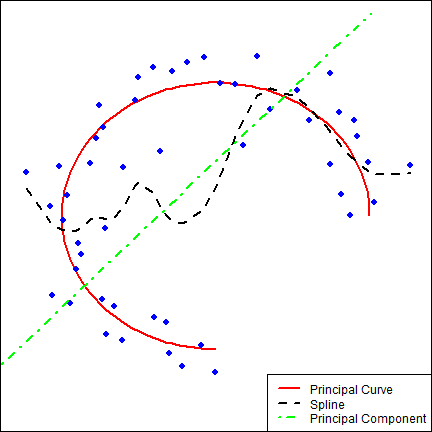
Though PCA is a widely used strategy for dimension reduction, it can lead to over simplification. As shown in the left panel in Figure 2, the underlying true curve that generates the data is part of a circle while the first principal component is a line. Direct applications of splines, wavelets and related regression methods cannot be done as they require the mean function of the data to be in a functional form; that is, there is only one $y$ for every $x$ . This is clearly violated in the corpus callosum example and many other white matter manifolds of interest. Palus and Dvorak [29] illustrated the pitfalls and precautions when applying linear PCA in non-linear settings. In our case, since the corpus callosum clearly is a nonlinear structure, PCA is not a viable candidate for dimension reduction.

Many non-linear methods have been proposed for fitting non-linear data structures. As an example, [10] proposed a non-linear extension of PCA. The core idea is to include product combinations of the variables in the data matrix. Another useful tool – the self-organizing map (SOM) – was proposed in [20], [21]. SOMs are unsupervised learning procedures which are used to discover structure in the data. Other nonlinear method methods such as non-linear principal component analysis (NLPCA) [23], [22] and principal geodesic analysis (PGA) [8], [7] can also fit non-linear data structures.

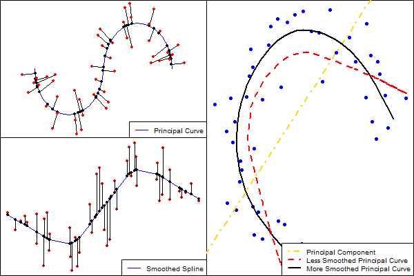
An important concept in doing non-linear data compression is principal surfaces [17], [18]. Principal surfaces are manifolds that pass through the middle of the data. The surfaces are fit via nonparametric low-dimensional manifolds that minimize the orthogonal distance from the data to themselves. Principal surfaces satisfy a self consistency condition, in that they are the conditional expectation (local average) of the data. The middle panel of Figure 2 shows the difference between the principal curves (surfaces) and regression. It highlights that the principal curve minimizes the sum of orthogonal distances while a spline model fit tries to minimize the sum of distances parallel to the y axis.

The principal surface is not unique. For example, it has been proven [17], [18] that all the principal components of a dataset are self-consistent. Other factors may also impact the results of fitting principal curves and surfaces. Using another example, different smoothness and lengths also lead to different principal curves. The original algorithm proposed in [18] used an iterated algorithm with local planar smoother to achieve the principal surfaces. Motivated by multivariate adaptive regression splines (MARS), adaptive principal surface is proposed later in [24]. Dong and McAvoy [4] combines principal curves and neural networks. The authors construct a principal curve via a two-step neural network where the nonlinear “layer” is the construction of principal curve. Einbeck et al. [6] proposed an algorithm for fitting local principal surfaces. The surface is connected via triangles and the main work is then to find adjacent vertices. Goldsmith et al.[12] proposed a tube fitting algorithm based on principal curve method. Other algorithms have been proposed recently, such as fitting principal surfaces via kernel map manifold (KMM methods) [9] and constructing local principal curves and surfaces using subspace constraint mean shift (SCMS) [27].

Some local search methods though could fit the principal surface, may not have equally spaced parametrization on the surface. This will definitely lead to poor visualization of the flattened surface. In addition, some previous work can only achieve locally planar surfaces while for corpus callosum and other white matter tracts, a surface with certain degree of smoothness would be more reasonable. Therefore, we develop a method of obtaining a smoothed principal surface of the data with better parametrization on the surface. The rest of the manuscript is laid out as follows: In section 2, the principal surface concept will be introduced, and its corresponding algorithm will be shown. We will show how the principal surface algorithm works on simulated data in section 3. The algorithm then is applied to corpus callosum data and the FA maps are obtained in section 4. We will conclude the whole paper in section 5.

2 Methods

2.1 Principal Surfaces

Let $\mathbf{x}_{i}=(x_{i1},x_{i2},x_{i3})^{T},\ i=1,\dots,I$ be the data points in three dimensional space, $\mathcal{R}^{3}$ following an underlying distribution. $\mathbf{t}_{i}=(t_{i1},t_{i2})^{T}$ be corresponding parametrization points in two dimensional space, $\mathcal{R}^{2}$ . In addition, we will require (without loss of generality) that the 2D coordinate space be the unit square $[0,1]\times[0,1]\subset\mathcal{R}^{2}$ . We define $f$ as the smooth principal surface function $f:\mathbf{t}_{i}\mapsto f(\mathbf{t}_{i})$ that maps from $\mathcal{R}^{2}$ to $\mathcal{R}^{3}$ . The principal surface function satisfies the self-consistency condition:

E(\mathbf{X}|\lambda_{f}(\mathbf{X})=\mathbf{t})=f(\mathbf{t})\ \ \text{for all }\mathbf{t},

(1)

where $\lambda_{f}(\mathbf{x})=\sup_{\mathbf{t}}\big\{\mathbf{t}:\|\mathbf{x}-f(\mathbf{t})\|=\inf_{\mathbf{\mu}}\|\mathbf{x}-f(\mathbf{\mu})\|\big\}$ is the projection function with respect to $f$ . The projection function maps a data point on to the closest principal surface point having the largest parametrization. Hastie and Stuetzle [18] showed that principal curves and surfaces generally exist, though are not unique. We have found that there are two main distinctions between different fitted principal surfaces: the degree of smoothness and the method of parametrization. In most algorithms, these properties will be controlled by the specific smoother being used in the algorithm and its tuning parameters. The details of our specific algorithm will be demonstrated in the next section.

2.2 Algorithm

In this paper, the algorithm used in [18] will be modified. This algorithm allows us to find the surface coordinate for each data point ( $\mathbf{t}_{i},i=1,\dots,I$ ), which we will use later to create parametric summaries. However, the original principal surface algorithm can only yield surfaces which are locally flattened. Therefore, instead of local planar smoothers, we employ thin-plate splines (TPS) for fitting the surface. Thin-plate splines were proposed by [5] and are now widely used for bivariate smoothing. The TPS penalize the least squares error by a high-order derivative term in order to achieve a desired degree of smoothness. Wood [32] improved the computational efficiency when fitting TPS by using an optimal approximating basis that we employ.

Preprocessing. Recall the notation we defined in section 2.2, let $\mathbf{X}=[\mathbf{x}_{1},\dots,\mathbf{x}_{I}]^{T}$ be the $I\times 3$ matrix that contains the 3D coordinates of the dataset. We assumed that the data are centered around the origin. Principal component decomposition is then applied. Let $\mathbf{X}=\mathbf{U}\mathbf{\Sigma}\mathbf{V}^{T}$ be the singular value decomposition of $\mathbf{X}$ . Then $\mathbf{U}\tilde{\mathbf{\Sigma}}$ are the first two principal “scores” of the data matrix, where $\tilde{\mathbf{\Sigma}}$ is a submatrix of $\mathbf{\Sigma}$ containing the first two columns. We then standardized the scores so that both scores are in $[0,\ 1].$ and used them as the initial 2D parametrization.

Conditional Expectation. Suppose $\mathbf{t}_{i}=(t_{i1},t_{i2})^{T}$ be the current parametrization of $\mathbf{x}_{i}$ in two dimensional space, $[0,1]\times[0,1]$ . For a specific data point $\mathbf{x}_{0}$ , with its coordinate $\mathbf{t}_{0}$ , we choose $r$ as a radius, such that all the other data points with their projection coordinate having less distance from $\mathbf{t}_{0}$ than $r$ are considered as the neighbor of $\mathbf{x}$ , see the left panel in Figure 3. Let $\mathcal{N}_{\mathbf{x}_{0}}$ be the set of all the neighbors of the point $\mathbf{x}_{0}$ . Then we have $\mathcal{N}_{\mathbf{x}_{0}}=\big\{\mathbf{x}_{j}:\ \|\mathbf{t}_{j}-\mathbf{t}_{0}\|\leq r\big\}$ and we calculate the local weighted average as follows:

\mathbf{x}^{lm}=\sum_{i}w^{\mathbf{x}}_{i}\mathbf{x}_{i}\ \ \text{where}\ \ w_{i}^{\mathbf{x}}:=\mathbf{1}_{[\mathbf{x}_{i}\in\mathcal{N}_{\mathbf{x}_{0}}]}\times\frac{\exp\big\{-\frac{\|\mathbf{t}_{i}-\mathbf{t}\|_{2}^{2}}{h}\big\}}{\sum_{j:\ \mathbf{x}_{j}\in\mathcal{N}_{\mathbf{x}_{0}}}\exp\big\{-\frac{\|\mathbf{t}_{j}-\mathbf{t}\|_{2}^{2}}{h}\big\}}.

Smoothing. Bivariate thin plate splines [32] are applied after we obtained these local averages: $\mathbf{x}_{i}^{lm},\ i=1,\dots,I$ . In this step, we fitted

x^{lm}_{id}=f_{d1}(t_{i1})+f_{d2}(t_{i2})+f_{d3}(t_{i1},t_{i2})+\epsilon_{id},\ \ d=1,2,3,

(2)

and obtained a bivariate thin plate spline smoothing of the local average points, which is demonstrated in the right panel of Figure 3. Here

f(\mathbf{t}_{i})=\left[\begin{array}[]{l}\hat{f}_{11}(t_{i1})+\hat{f}_{12}(t_{i2})+\hat{f}_{13}(t_{i1},t_{i2})\\ \hat{f}_{21}(t_{i1})+\hat{f}_{22}(t_{i2})+\hat{f}_{23}(t_{i1},t_{i2})\\ \hat{f}_{31}(t_{i1})+\hat{f}_{32}(t_{i2})+\hat{f}_{33}(t_{i1},t_{i2})\end{array}\right]

(3)

is the current principal surface function mapping from the 2D parametrization space to 3D coordinate space. The thin plate splines could be fitted using “mgcv” package in software R.

Projection. We then projected each data point onto the current principal surface and obtained new 2D parametrization. we used a grid search method to find the projection and only search within the range $[0,1]\times[0,1]$ . Therefore there will be some data points being projected onto the boundary, which brings some issues when we further analyzed the 2D parametrization. After this step, we iterated the whole procedure with the new 2D parametrization.

The whole algorithm is illustrated as follows:

Input: Data in 3D coordinate,

\mathbf{X}_{I\times 3}

Output: Principal surface function,

f_{\mathcal{R}^{2}\to\mathcal{R}^{3}}

, and the 2D parametrization of all data points,

\mathbf{T}_{I\times 2}

Initialization: De-mean

\mathbf{X}

for each column;

set the initial 2D parametrization as

\mathbf{T}^{(0)}=\mathbf{U}\tilde{\mathbf{\Sigma}}

;

Set err

=1

, i

=1

;

while ( $i$ $<$ max.iter and err $>$ thres) do

(1).

\mathbf{X}^{lm}\longleftarrow\mathbf{W}\mathbf{X}

, where

w_{ij}=\mathbf{1}_{[\mathbf{x}^{(i)}\in\mathcal{N}_{\mathbf{x}^{(j)}}]}w_{j}^{(\mathbf{x}_{i})}

;

(2). Fit

\mathbf{X}^{lm}=f(\mathbf{T})+\mathbf{\epsilon}

;

(3).

\mathbf{t}^{(new)}_{i}\longleftarrow arg\min_{\mathbf{t}}\|\mathbf{x}_{i}-f(\mathbf{t})\|^{2}

;

(4).

err\longleftarrow\|\mathbf{T^{old}}-\mathbf{T^{(new)}}\|_{2}^{2},\ i\longleftarrow i+1

;

end while

Algorithm 1 Principal surface algorithm

3 Simulation Results

3.1 Simulation Setup

We illustrate four examples to investigate the algorithm in highly idealized test settings. The number of data points was set to $I=6,000$ in all simulation settings and we sampled a subset of $1,000$ points in each case. The data were centered around $(0,0,0)$ , which was assumed known.

Case 1 The data points in the first simulation case are uniformly distributed around a cylinder with an open seam. Set $\theta_{i}\sim U(0,2\pi-0.5)$ , $\epsilon_{i}\sim N(0,0.15^{2})$ and $z_{i}\sim U(-3,3)$ i.i.d., then let

\mathbf{x}_{i}=\left[\begin{array}[]{c}\cos{\theta_{i}}(1+\epsilon_{i})\\ \sin{\theta_{i}}(1+\epsilon_{i})\\ z_{i}\end{array}\right].

Case 2 The second case is based on the Himmelblau’s function [19], which is $f(x,y)=(x^{2}+y-11)^{2}+(x+y^{2}-7)^{2}$ . Let $z_{i1}\sim U(-5,5)$ , $z_{i2}\sim U(-5,5)$ , $\epsilon_{i}\sim N(0,50^{2})$ i.i.d., then let

\mathbf{x}_{i}=\left[\begin{array}[]{c}z_{i1}\\ z_{i2}\\ -\frac{1}{100}\big\{(z_{i1}^{2}+z_{i2}-11)^{2}+(z_{i1}+z_{i2}^{2}-7)^{2}+\epsilon_{i}\big\}\end{array}\right].

Case 3 In the third case the data points form a flatten surface at the beginning and then begin to bent over towards the bottom. Set $z_{i1}\sim U(0,2)$ , $z_{i3}=0$ when $i=1,\dots,I/2$ ; $z_{i1}=\cos(\theta_{i})+2$ , $z_{i3}=-1+\sin(\theta_{i})$ for $i=I/2+1,\dots,I$ , where $\theta_{i}\sim U(-\pi/2,\pi/2)$ . Let $z_{i2}\sim U(0,10)$ and $\epsilon_{i}\sim U(-0.4,0.4)$ . All the random numbers are generated independently. Then we let

\mathbf{x}_{i}=\left[\begin{array}[]{c}z_{i1}\\ z_{i2}\\ z_{i3}+\epsilon_{i}\end{array}\right].

Case 4 In the last case, we produce a two dimensional stretched digit “5”. Let $z_{i1}\sim U(0,1)$ , $z_{i3}=0$ when $i=1\dots,3I/10$ ; $z_{i1}=0$ , $z_{i3}\sim U(-1,0)$ when $i=3I/10+1,\dots,4.5I/10$ ; $z_{i1}\sim U(0,0.5)$ , $z_{i3}=-1$ when $i=4.5I/10+1,\dots,6I/10$ ; $z_{i1}=\frac{1}{2}+\frac{1}{2}\cos(\theta_{i})$ , $z_{i3}=-\frac{3}{2}+\frac{1}{2}\sin(\theta_{i})$ for $i=6I/10+1,\dots,8.5I/10$ where $\theta_{i}\sim U(-\pi/2,\pi/2)$ ; $z_{i1}\sim U(0,0.5)$ , $z_{i3}=-2$ when $i=8.5I/10+1,\dots,I$ . Let $z_{i2}\sim U(0,5)$ and $\epsilon_{i}\sim U(-0.15,0.15)$ when $i=1,\dots,I$ . All the random numbers are generated independently. Then we let

\mathbf{x}_{i}=\left[\begin{array}[]{c}z_{i1}+\epsilon_{i}\\ z_{i2}\\ z_{i3}+\epsilon_{i}\end{array}\right].

3.2 Simulation Results

The results of the principal surface fitting algorithm for four examples are shown in Figure 4. Starting in the upper left panel in Figure 4, one can see that the algorithm reconstructs the cylinder very well. Since we did not force any constraints in fitting the surface, we do not achieve a closed seam cylinder. (Finding principal surfaces for closed cylinders or spheres remains an interesting topic for future research.) Other upper panels illustrate the fitting results of the Himmelblau’s function, a non-function shaped “carpet” data cloud and a simulated digit “5” data cloud. The four panels in the bottom panels in Figure 4 compare the fitted surfaces with the original surfaces that generate the data cloud. The result are satisfactory for all cases. Given that the desired corpus callosum model fit is far simpler and smoother than these examples, the simulations show evidence of the viability of the principal surface algorithm as a robust method for this problem.

For all four scenarios, the algorithm converged in less than 20 steps and took under two minutes on a i3-2.3GHz PC machine with 4Gb RAM memory. To further investigate practical computing speed, we set varied sample sizes and number of grid points ( $N_{grid}$ ) for the third case above and measured the iterations and compute time. The results are illustrated in Table 1. As the number of grid points or the number of data points increases, the computing time for each iteration step increases correspondingly, though did not go out the range of reasonable compute times. Note that, one would rarely use the entire dataset in large sample size cases. Our recommended strategy is to take random subsamples from the dataset and subsequently fit the surface using the subsample, if necessary, repeating the sub-sampling to investigate its impact on model fits. In addition, as the grid number increases, the number of steps to attain convergence decreases.

4 Application

4.1 Fitting the Principal Surface of a Corpus Callosum

The data contain 466 scans generated from a diffusion tensor imaging (DTI) experiment performed on 176 MS patients. For each scan, we have corresponding fractional anisotropy (FA) value for each voxel of the entire corpus callosum area extracted via tractography. More detailed data description are provided in [30] and [28]. Fractional anisotropy has been associated cross sectionally and longitudinally with multiple sclerosis diagnoses and symptoms [11], [15], [16], [30], [35]. Ignoring the FA value for the moment, we first discuss the principal surface fit.

For each scan, there are roughly 20,000 data points in the corpus callosum region of interest. For computational simplicity, we randomly choose 1,000 of them to build the surface. We illustrate the result of four scans as well as the overall average fitted surface in the left panels in Figure 5. The fitted surface for each scan is reasonable and is indicative of the fits from the other scans, each inspected visually. The overall average is smoother than each scan as we expected.

4.2 Flattened FA Representation

A primary goal from the principal surface fitting is to flatten the surface and to make a 2D FA image. That is, our goal is to use DTI-based morphometric information to create 2D images of MR contrast properties, such as FA maps. First, we project each data point onto the surface by a grid search method. Then we smooth the associated FA value on the surface by calculating a local average. Interpolating this smooth onto a grid yields a $100\times 100$ 2D FA image displayed in the right panels of Figure 5. That is, right panels represent the flattened surfaces of the corresponding left panels. The bottom panel shows the average FA map, which shows an overall visualization of 2D FA maps for all the scans. Another important fact is from left panels in Figure 5 and right panel in Figure 1, we can see that important information of the FA values is retained, which is to say, it may be sufficient to visualize the 2D FA values instead of the original 3D FA values.

5 Discussion

In this manuscript we introduced a principal surface algorithm and used it to fit the corpus callosum. The goal of this work is largely developmental, creating a handy tool for dimension reduction in DTI analysis of a primary structure. The result of both the simulations and the application is encouraging. While applied to the corpus callosum, the algorithm could be applied to any other three dimensional manifold-like objects where a two dimensional surface could be embedded and is of interest, for example, all the major white matter tracts in the brain [1]. The two dimensional manifold characterizes the original data and accomplishes both dimension reduction and better visualization. The surface that we constructed is smooth and could be easily projected onto to represent other properties of the original structure, such as the FA, mean diffusivity, parallel diffusivity, local thickness and so on. The algorithm is computationally feasible and scales well to larger images and densely measured structures.

The role of the two dimensional sub-representation needs to be further explored. For future work, we are developing functional data analysis tools [11], [14], [16], [34], [33] for relating the dimension reduced 2D manifold to outcomes of interest for the purpose of inference, biomarker creation and prediction. Of note, we are particularly interested in whether or not the 2D representation of the corpus callosum is less sensitive to issues of whole brain registration often used in the processing pipeline. In fact, it is possible that registering the 2D representation is preferable to whole brain registration a priori in certain applications. We note also that MFPCA [3] and LFPCA [35] methods have been shown to isolate registration error as a part of the model [25], thus raising the intriguing possibility of DTI processing streams that dramatically decrease the need and importance of whole brain template-based registration.

Furthermore, current works suggest sagittal mid-line callosum average thickness might be of very meaningful in the study of some diseases [26], [31]. In contrast, The principal surface approach allows us to calculate the local thickness over the main body of the structure. We then could construct a global thickness map for the whole corpus callosum, following a procedure similar to that of constructing the FA map. Based on this, the thickness changes of white matter could be measured on the whole corpus callosum instead of the mid-sagittal slice.

Finally, we note that the procedure that we proposed can be further extended as a general problem of fitting skeleton manifolds. First, we are interested in fitting surfaces with fixed boundaries. Work has been done to analyze principal curves with fixed starting and ending points [2]. The extension to surfaces would be challenging. Suppose $\b{t}=(t_{1},t_{2})$ is the corresponding coordinate on the surface of the original data point, $\b{x}=(x_{1},x_{2},x_{3})$ , which lies in 3D space. We restrict the range of $\b{t}$ to be $[0,1]\times[0,1]$ . Now consider a predetermined function for $\b{x}(\b{t})=(x_{1}(\b{t}),x_{2}(\b{t}),x_{3}(\b{t}))$ when the boundary values of $t$ are linearly constrained. Such constraints would yield cylindrical fits easily though extensions to completely closed surfaces would require more elaborate constraints.

6 Acknowledgements

The project described was supported by Grant Number R01EB012547 and NIH grant P41 EB015909 from the National Institute of Biomedical Imaging And Bioengineering. The project described was also supported by Grant Number R01NS060910 from the National Institute of Neurological Disorders and Stroke. Data for this study was acquired with grants from the National Multiple Sclerosis Society and EMD Serono.

Appendix A Figures

Refer to caption — Figure 1: Left panel: 3D-rendering of corpus callosum. Right panel: horizontal, sagittal, and coronal slices. Views: R=Right, L=Left, S=Superior, I=Interior, A=Anterior, P=Posterior. Produced in 3DSlicer (4.1.1)

Appendix B Tables

Table 1: Simulation computing time consuming comparison

Sample	Number of grid points, denoted as $N_{grid}$
	15	30	50	100	15	30	50	100	15	30	50	100
Size	Total time usage (Sec.)				Number of iterations				Time per iteration (Sec.)
100	4	4	4	8	6	5	3	3	1	1	1	3
200	7	5	5	10	11	6	4	3	1	1	1	3
500	18	12	11	20	17	8	5	4	1	1	2	5
700	27	21	18	32	20	12	7	5	1	2	3	6
1000	39	40	35	49	22	15	10	6	2	3	3	8

References

[1] Pierre-Louis Bazin, Chuyang Ye, John A. Bogovic, Navid Shiee, Daniel S. Reich, Jerry L. Prince, and Dzung L. Pham. Direct segmentation of the major white matter tracts in diffusion tensor images. NeuroImage, 58(2):458 – 468, 2011.
[2] Brian S. Caffo, Ciprian M. Crainiceanu, Lijuan Deng, and Craig W. Hendrix. A case study in pharmacologic imaging using principal curves in single photon emission computed tomography. Johns Hopkins University, Dept. of Biostatistics Working Papers, 143, 2007.
[3] C. Di, C. Crainiceanu, B. Caffo, and N. Punjabi. Multilevel functional principal component analysis. Annals of Applied Statistics, 3(1):458–488, 2009.
[4] D. Dong and T.J. McAvoy. Nonlinear principal component analysis based on principal curves and neural networks. Computers Chemical Engineering, 20(1):65 – 78, 1996. ISSN 0098-1354.
[5] J. Duchon. Splines minimizing rotation-invariant semi-norms in soboley spaces. Lecture notes in mathematics, 571/1977:85–100, 1977.
[6] J. Einbeck, L. Evers, and B. Powell. Data compression and regression through local principal curves and surfaces. International journal of neural systems, 20(3):177–192, 2010.
[7] P.T. Fletcher. Statistical variability in nonlinear spaces: Application to shape analysis and dt-mri phd thesis, university of north carolina at chapel hill. 2004.
[8] P.T. Fletcher, Conglin Lu, S.M. Pizer, and Sarang Joshi. Principal geodesic analysis for the study of nonlinear statistics of shape. Medical Imaging, IEEE Transactions on, 23(8):995 –1005, aug. 2004. ISSN 0278-0062.
[9] S. Gerber, T. Tasdien, and R. Whitaker. Dimensionality reduction and principal surfaces via kernel map manifolds. Computer Vision, 2009 IEEE 12th International Conference, pages 529–536, 2009.
[10] H Gnanadesikan. Methods for Statistical Analysis of Multivariate Observations. Wiley, New York, 1997.
[11] J. Goldsmith, J. Feder, C.M. Crainiceanu, B. Caffo, and D. Reich. Penalized functional regression. Johns Hopkins University, Dept. of Biostatistics Working Papers, page 204, 2010.
[12] J. Goldsmith, B. Caffo, C. Crainiceanu, D. Reich, Y. Du, and C. Hendrix. Nonlinear tube-fitting for the analysis of anatomical and functional structures. The annals of applied statistics, 5(1):337–363, 2011a.
[13] J. Goldsmith, C.M. Crainiceanu, B.S. Caffo, and D.S. Reich. Penalized functional regression analysis of white-matter tract profiles in multiple sclerosis. NeuroImage, 2011b.
[14] J. Goldsmith, M.P. Wand, and C. Crainiceanu. Functional regression via variational bayes. Electronic Journal of Statistics, 5:572–602, 2011c.
[15] J. Goldsmith, C.M. Crainiceanu, B. Caffo, and D. Reich. Longitudinal penalized functional regression for cognitive outcomes on neuronal tract measurements. Journal of the Royal Statistical Society: Series C (Applied Statistics), 2012.
[16] S. Greven, C. Crainiceanu, B. Caffo, and D. Reich. Longitudinal functional principal component analysis. Recent Advances in Functional Data Analysis and Related Topics, pages 149–154, 2011.
[17] T. Hastie. Principal curves and surfaces. Technical report, 11, 1984.
[18] T. Hastie and W. Stuetzle. Principal curves. Journal of the American Statistical Association, 84(406):502–516, 1989.
[19] David M. Himmelblau. Applied nonlinear programming. McGraw-Hill (New York), 1972.
[20] T. Kohonen. The self-organizing map. Proceedings of the IEEE, 78(9):1464 –1480, sep 1990. ISSN 0018-9219.
[21] Teuvo Kohonen. Self-organized formation of topologically correct feature maps. Biological Cybernetics, 43:59–69, 1982. ISSN 0340-1200.
[22] Mark A. Kramer. Nonlinear principal component analysis using autoassociative neural networks. AIChE Journal, 37(2):233–243, 1991. ISSN 1547-5905.
[23] Mark A. Kramer. Autoassociative neural networks. Computers and Chemical Engineering, 16(4):313 – 328, 1992. ISSN 0098-1354. Neutral network applications in chemical engineering.
[24] Michael Leblanc and Robert Tibshirani. Adaptive principal surfaces. Journal of the American Statistical Association, 89(425):53–64, 1994.
[25] S Lee, V Zipunnikov, B Caffo, D Reich, and D Pham. Statistical image analysis of longitudinal ravens images: methodology and case study. Technical Report, 2012.
[26] Eileen Luders, Katherine L. Narr, Liberty S. Hamilton, Owen R. Phillips, Paul M. Thompson, Jessica S. Valle, Melissa Del’Homme, Tony Strickland, James T. McCracken, Arthur W. Toga, and Jennifer G. Levitt. Decreased callosal thickness in attention-deficit/hyperactivity disorder. Biological Psychiatry, 65(1):84 – 88, 2009.
[27] U. Ozertem and D. Erdogmus. Locally defined principal curves and surfaces. Journal of Machine learning research, 12:1249–1286, 2011.
[28] A. Ozturk, SA Smith, EM Gordon-Lipkin, DM Harrison, N. Shiee, DL Pham, BS Caffo, PA Calabresi, and DS Reich. Mri of the corpus callosum in multiple sclerosis: association with disability. Multiple Sclerosis, 16(2):166–177, 2010.
[29] Milan Palus and Ivan Dvorak. Singular-value decomposition in attractor reconstruction: Pitfalls and precautions. Physica D: Nonlinear Phenomena, 55(12):221 – 234, 1992. ISSN 0167-2789.
[30] D. Reich, A. Ozturk, P. Calabresi, and S. Mori. Automated vs. conventional tractography in multiple sclerosis: Variability and correlation with disability. NeuroImage, 49:3047–3056, 2010.
[31] C.N. Vidal, R. Nicolson, T.J. DeVito, K.M. Hayashi, J.A. Geaga, D.J. Drost, P.C. Williamson, N. Rajakumar, Y. Sui, R.A. Dutton, et al. Mapping corpus callosum deficits in autism: an index of aberrant cortical connectivity. Biological Psychiatry, 60(3):218–225, 2006.
[32] S. Wood. Thin plate regression splines. Journal of the royal statistical society, 65(1):95–114, 2003.
[33] H. Zhu, M. Styner, N. Tang, Z. Liu, W. Lin, and J.H. Gilmore. Frats: Functional regression analysis of dti tract statistics. Medical Imaging, IEEE Transactions on, 29(4):1039–1049, 2010.
[34] H. Zhu, L. Kong, R. Li, M. Styner, G. Gerig, W. Lin, and J.H. Gilmore. Fadtts: Functional analysis of diffusion tensor tract statistics. NeuroImage, 56(3):1412–1425, 2011.
[35] Vadim Zipunnikov, Sonja Greven, Brian Caffo, Daniel S. Reich, and Ciprian Crainiceanu. Longitudinal high-dimensional data analysis. Johns Hopkins University, Dept. of Biostatistics Working Papers, 234, 2011.