Incremental Computation of Pseudo-Inverse of Laplacian
Theory and Applications
Abstract
A divide-and-conquer based approach for computing the Moore-Penrose pseudo-inverse of the combinatorial Laplacian matrix of a simple, undirected graph is proposed. The nature of the underlying sub-problems is studied in detail by means of an elegant interplay between and the effective resistance distance . Closed forms are provided for a novel two-stage process that helps compute the pseudo-inverse incrementally. Analogous scalar forms are obtained for the converse case, that of structural regress, which entails the breaking up of a graph into disjoint components through successive edge deletions. The scalar forms in both cases, show absolute element-wise independence at all stages, thus suggesting potential parallelizability. Analytical and experimental results are presented for dynamic (time-evolving) graphs as well as large graphs in general (representing real-world networks). An order of magnitude reduction in computational time is achieved for dynamic graphs; while in the general case, our approach performs better in practice than the standard methods, even though the worst case theoretical complexities may remain the same: an important contribution with consequences to the study of online social networks.
1 Introduction
The combinatorial Laplacian matrix of a graph finds use in various aspects of structural analysis [4, 18, 19, 24, 25, 28, 30, 37, 38, 39, 41, 50, 34]. The eigen spectrum of the Laplacian determines significant topological characteristics of the graph, such as minimal cuts, clustering and the number of spanning trees [9, 24, 25, 34]. Likewise, the Moore-Penrose pseudo-inverse and the sub-matrix inverses of the Laplacian have evoked great interest in recent times. Their applications span fields as diverse as probability and mathematical chemistry, collaborative recommendation systems and social networks, epidemiology and infrastructure planning [28, 31, 32, 33, 40, 46, 55]. A brief discussion of the specific applications is provided for reference in a subsequent section (c.f. §6). Alas, despite such versatility, the pseudo-inverse and the sub-matrix inverses of the Laplacian suffer a practical handicap. These matrices are notoriously expensive to compute. The standard matrix factorization and inversion based methods employed to compute them [8, 55], incur an computational time, being the order of the graph (number of vertices in the graph). This clearly impedes their utility particularly when the graphs are either dynamic, i.e. changing with time, or simply of large orders, i.e. have millions of nodes. Online social networks , typically represented as graphs, qualify on both counts. With time, the number of users as well as the relationships between them changes, thus requiring regular re-computations. As for size, a popular OSN, such as Facebook and Youtube, may easily have hundreds of millions of users. An cost, therefore, is clearly undesirable and an approach for incremental updates is imperative, particularly given that such changes, in most cases, may be local in nature.
In this work, we provide a novel divide-and-conquer based approach for computing the Moore-Penrose pseudo-inverse of the Laplacian for an undirected graph which, in turn, determines all of its sub-matrix inverses as well. The divide operation in our approach entails determining an arbitrary connected bi-partition of the graph — a cut of the graph that is made up of exactly two connected sub-graphs (say and ) — by deleting edges from it. As and are simple and connected themselves, the pseudo-inverse of their Laplacians, when computed, constitute solutions to two independent sub-problems. Better still, they can be computed in parallel (given two machines instead of one). In the conquer step, we recombine these solutions in an iterative manner by re-introducing the edges in the cut set one at a time to reconstruct the original graph and obtain the overall pseudo-inverse in the process. Note that, this process yields a sequence of intermediate spanning sub-graphs of , (say ), where . The first transition represents a point of singularity in our method whence the disjoint components get connected through a bridge edge to yield , a sub-graph with exactly one component. We call this stage the first join in our process. Post the first join, all intermediate sub-graphs from to are obtained by introducing an edge in a sub-graph that is already connected. We call this edge firing (details in a subsequent section). We then show that the pseudo-inverse of the Laplacian for any intermediate sub-graph in this sequence is determined entirely in terms of the pseudo-inverse of the Laplacian for its predecessor. Our results, presented in an element-wise scalar form, reveal several interesting properties of the sub-problems. First and foremost, if be the order of the graph , then the cost incurred at each intermediate stage is if the solution to the sub-problems for the immediate predecessor is known. Therefore, the cost of computing the pseudo-inverse for is , if the pseudo-inverses for and are known. Secondly, using these forms, each element of the pseudo-inverse for an intermediate graph can be computed independent of the other elements. Hence, given multiple machines, the overall computational time is reduced further through parallelization. Moreover, we obtain similar closed form solutions for the case of structural regress of the graph, i.e. when vertices or edges are deleted from it. A straightforward consequence is that the pseudo-inverses for dynamic time-evolving graphs, such as OSNs, can now be updated when a node joins or leaves the network or an edge (a relationship) appears/disappears in it, at an cost overall (as ).
Last but not least, we use these insights to compute the pseudo-inverses of the Laplacians of large real-world networks from the domain of online social networks. Real-world networks, and social ones in particular, are reported to have some notable characteristics such as edge sparsity, power-law and scale-free degree distributions [7, 3, 22], small-world characteristics [54] etc. Given these properties, we note that interesting algorithms (heuristics) can be developed for fast and parallel computations for the general case based on our divide-and-conquer strategy. Thus, even though the theoretical worst case costs stay at for general graphs, the practical gains are significant enough to warrant attention. We discuss both analytical and experimental aspects of these in detail in the subsequent sections.
The rest of the paper is organized into the following sections: we begin by introducing the preliminaries of our work — the pseudo-inverse and the sub-matrix inverses of the Laplacian along with their properties; and the interplay of the pseudo-inverse and the effective resistance distance — in §2. In §3, we describe our divide-and-conquer strategy involving connected bi-partitions and the two-stage process for computing the Moore-Penrose pseudo-inverse of the Laplacian. Relevant scalar forms are presented in each case. In §4, we establish the same closed forms for a graph in regress i.e. deleting edges one at a time until the graph breaks into two. We then apply the divide-and-conquer methodology to compute the pseudo-inverses for dynamically changing graphs as well as those of real world networks in §5. In §6 we briefly overview related literature discussing specific application scenarios. The paper is finally concluded in §7 with a summary of results and a discussion of potential future works.
2 The Laplacian, Sub-Matrix Inverses and A Distance Function
In this section, we provide a brief introduction to the set of matrices studied in this work, namely, the combinatorial Laplacian of a graph (), its Moore-Penrose pseudo-inverse () and the set of sub-matrix inverses of (§2.1). We then demonstrate how all the sub-matrix inverses of the Laplacian can be computed in terms of the pseudo-inverse in §2.2. Finally, in §2.3 we describe the relationship between the effective resistance distance, a Euclidean metric, and the elements of the Moore-Penrose pseudo-inverse of the Laplacian — an equivalence that we exploit to great advantage in the rest of this work.
2.1 The Laplacian and its Moore-Penrose Pseudo-Inverse
Let be a simple, connected and undirected graph. We denote by the number of nodes/vertices in , also called the order of the graph , and by the number of links/edges. The adjacency matrix of is defined as , with elements , if and is an edge; otherwise. Here, the weight of the edge is a measure of affinity between nodes and . Clearly, is real and symmetric. The degree matrix , is a diagonal matrix where , is the weighted degree of node ; the sum of all edge weights (affinities) emanating from . Also, , is called the volume of the graph — the sum total of affinities between all pairs of vertices in . The combinatorial Laplacian of the graph is then given by:
| (1) |
It is easy to see, from the definition in above, that the Laplacian is a real, symmetric and doubly-centered matrix (each row/column sum is 0). More importantly, admits an eigen decomposition of the form where the columns of constitute the set of orthogonal eigen vectors of and is a diagonal matrix with ; being the eigen values of . It is well established that for a connected undirected graph , is positive semi-definite i.e. it has a unique smallest eigen value . The rest of the eigen values are all positive. Thus, is rank deficient () and consequently singular. Its inverse, in the usual sense, does not exist.
However, the Moore-Penrose pseudo-inverse of , denoted henceforth by does exist and is unique. Following constitute the basic properties of as a unique generalized inverse of [8]:
| (2) |
Like , is also real, symmetric, doubly centered and positive semi-definite. Moreover, the eigen decomposition of is given by , with the same set of orthogonal eigen-vectors as that of . The set of eigen values of , given by the diagonal of the matrix , is composed of and the reciprocals of the positive eigen-values of . We denote by , the element in the row and column of (a convention followed for all matrices henceforth). We emphasize that even when the matrix is sparse (which is the case with real world networks), is always a full matrix. In fact, for a connected graph, all the elements of are non-zero.
A straightforward approach for computing is through the eigen-decomposition of , followed by an inversion of its non-zero eigen values, and finally reassembling the matrix as discussed above. In practice, however, mathematical software, such as MATLAB, use singular value decomposition to compute the pseudo-inverse of matrices (c.f. in the standard library). This general SVD based method does not exploit the special structural properties of and incurs computational time, being the number of nodes in the graph. An alternative has recently been proposed in [55] specifically for computing for a simple, connected, undirected graph. A perturbation of the matrix makes it invertible. can then be computed from this perturbed matrix as follows:
| (3) |
where is a matrix of all . Although the theoretical cost for this method is also , in practice it works faster for graphs of arbitrary orders and edge densities than the standard method. But the proof of this pudding is in computing! So, to put into context the notion, we present a numerical analysis over Erdös-Rényi graphs (ER-graphs) of varying orders and edge densities. An ER-graph is a random graph determined by parameters , where is the order of the graph and is the uniform probability for the occurrence of any arbitrary (undirected) edge in the graph [11]. We use a dedicated machine with a quad-core AMD Opteron processor and of primary memory.
Fig. 1 shows a comparison of the two methods for and . The experiment is repeated 100 times for each parametric combination . The fact that the method from [55] outperforms is self evident, as is the fact that the computational times for both methods rises with increasing values of . We also observe great consistency (or very little variance) across the different instances for a given , which is not too surprising. What is of interest, however, is that the computational times for a given value of do not vary significantly across , for either of the two methods. We observe the same for higher values of (not shown here). This implies that the methods are insensitive to the sparsity of the graphs. Moreover, for graphs of , the primary memory imprint for both methods is over when run in MATLAB (a little higher, in fact, for the perturbed inversion method). Although the exact figures may vary from machine to machine, they provide a rough estimate that suffices for the problem at hand. In summary, for dynamically changing graphs, in which small local modifications occur every now and then, such methods would incur undue heavy computational costs due to repeated re-computation of from scratch. On the other hand, for graphs of higher orders (), such decomposition/inversion based methods are rendered impractical from the point of view of computational time as well as memory requirements, if performed on a single machine.
In what follows, we show that the computation of the Moore-Penrose pseudo-inverse of the Laplacian can be done in a divide-and-conquer fashion. Our method allows efficient incremental updates of for dynamically changing graphs, without having to compute all over again. Moreover, computing for large graphs becomes feasible, in principle, through parallelization of (smaller) independent sub-problems over multiple machines, which can then be re-combined at cost per edge across a division (details in a subsequent section). But first we need to establish a few more preliminary results to further motivate our study.

 (a)
(b)
(a)
(b)
2.2 Sub-Matrix Inverses of
As described in the previous section, the combinatorial Laplacian of a connected graph , is singular and thus non-invertible. However, given that its rank is , any combination of columns (or rows) of constitutes a linearly independent set. Hence, any sub-matrix of is invertible. Indeed, the inverses of such sub-matrices are made use of in several graph analysis problems: enumerating the spanning trees and spanning forests of the graph [32], determining the random-walk betweenness of the nodes of the graph [40], to name a few. However, the cost of computing an sub-matrix inverse is still . To compute all such sub-matrix inverses amounts to a time complexity of . In the following, we show how they can be computed efficiently through .
Theorem 1
Let be an sub-matrix of formed by removing the row and column of . Then :
| (4) |
The result in Theorem 1 above expresses, in scalar form, the general element ( row, column) of the inverse of the sub-matrix in terms of the elements of , as claimed. As the choice of the row and column is arbitrary, we can see that the result holds in general for any sub-matrix (permuting the rows and columns of as per need). The cost of computing for a given vertex is . Therefore, all sub-matrix inverses can be computed in time from , which itself can be computed in time, even if the standard methods are used. This is clearly an order of magnitude improvement. Henceforth, we focus entirely on .
2.3 The Effective Resistance Distance and

An interesting analogy exists between graphs and resistive electrical circuits [20, 28, 33]. Given a simple, connected and undirected graph , the equivalent electrical network of the graph can be formed by replacing each edge , of weight with an electrical resistance (c.f. Fig. 2). A distance function can then be defined between any pair of nodes in the resulting EEN as follows:
Definition 1
Effective Resistance (): The voltage developed between nodes x and y, when a unit current is injected at node x and is withdrawn at node y.
It is well established that the square root of the effective resistance distance () is a Euclidean metric with interesting applications [28, 33]. Amongst other things, it determines the expected length of random commutes between node pairs in the graph: , [14, 52]. More importantly, can be expressed in terms of the elements of as follows:
| (5) |
We now invert the elegant form in (5) to derive an important result in the following lemma which gives us the general term of in terms of the distance function .
Lemma 1
| (6) |
The in Lemma 1 above is composed of two terms: a triangle inequality of effective resistances [52] and a double summand over all pairwise effective resistances in the EEN. It is easy to see that the double-summand simply reduces to a scalar multiple of the trace of (). Thus the functional half that determines the elements of , is the triangle inequality of the effective resistances, while the double summand contributes an additive constant to all the entries of . We illustrate the utility of this result, with the help of two kinds of graphs on the extremal ends of the connectedness spectrum: the star and the clique.11 1 The graphs in these examples are assumed to be unweighted, i.e. all edges have a unit resistance/conductance.
2.3.1 The Star
A star of order is a tree with exactly one vertex of degree , referred to as the root, and pendant vertices each of degree , called leaves, (c.f. Fig. 3). By definition, a singleton isolated vertex is also a degenerate star albeit with no leaves. It is easy to see that , being a tree, is the most sparse connected graph of order (with exactly edges). Also, is the most compact tree of its order (lowest diameter). In the following, we show how can be computed using the result of Lemma 1.
Corollary 1
For a star graph of order , with node as root and nodes as leaves, is given by:
| (7) |
| (8) |

2.3.2 The Clique
On the other end of the connectedness spectrum lies the clique. A clique of order is a complete graph with edges. Clearly, the clique is the densest possible graph of order , as there is a direct edge between any pair of vertices in it. It is also the most compact graph of its order (lowest diameter). Then,
Corollary 2
For a clique of order , is given by:
| (9) |
The results in the corollaries presented above are not just illustrative examples. They are also of interest from a computational point of view, particularly when the graph under study is an unweighted one. Both stars and cliques can occur as motif sub-graphs in any given graph. Indeed, for any non-trivial connected simple graph of order , there is at least one sub-graph that is a star. Selecting any vertex with , and conducting a one-hop breadth first search, generates a star sub-graph. Cliques, though not so universal, also occur in real world networks (e.g. citation networks). Therefore, in any divide-and-conquer methodology, both stars and cliques are likely to be found at some stage. We have already established that the cost of computing and is (as they are determined entirely by ) and hence the solution to such a sub-problem, when found, is obtained at the lowest possible cost — a true practical gain.
To conclude, we have demonstrated that there exists a relationship between the elements of and the pairwise effective resistances in the graph , that yields interesting closed form solutions for the pseudo-inverse for special graphs such as stars and cliques. In the subsequent sections, we demonstrate that it can be used to compute for general graphs as well, incrementally, in a divide-and-conquer fashion.
3 From Two to One: Computing by Partitions

In this section, we present our main result — the computation of the Moore-Penrose pseudo-inverse of the Laplacian, or , by means of graph bi-partitions. In §3.1, we lay out a two-stage process — the first join followed by edge firings — that underpins our methodology. We then provide specific closed form solutions in §3.2.
3.1 Connected Bi-Partitions of a Graph and the Two-Stage Process
In order to compute the Moore-Penrose pseudo-inverse of the Laplacian of a simple, connected, undirected and unweighted graph by parts, we must first establish that the problem can be decomposed into two, or more, sub-problems that can be solved independently. The solutions to the independent sub-problems can then be combined to obtain the overall result. But before we proceed to do so, a few notations are in order.
Definition 2
Connected Bi-partition : A cut of the graph which contains exactly two mutually exclusive and exhaustive connected sub-graphs and .
Fig. 4(a-b), shows a graph and a connected bi-partition of it, obtained from the graph by removing the set of dotted edges shown. Each partition has certain defining characteristics in terms of the set of vertices as well the set of edges in the graph. Let, and be the mutually exclusive and exhaustive subsets of i.e. and . Similarly, let and be the sets of edges in the respective sub-graphs and of and , the set of edges that violate the partition i.e. have one end in and the other in . Thus, and . We denote by , the set of all such connected bi-partitions of the graph .
It is easy to see that for an arbitrary connected bi-partition both and are themselves simple, connected, undirected and unweighted graphs. Hence, the discussion in §2 is applicable in its entirety to the sub-graphs and independently. Note then that and , the Moore-Penrose pseudo-inverse of the Laplacians of the sub-graphs and , must, by definition, exist. The pair , , constitutes the solution to two independent sub-problems represented in the set . All that remains to be shown now is that , can indeed be combined to obtain . It is this aspect of the methodology, that we call the two-stage process, as explained in detail below.
The original graph can be thought of, in some sense, as a bringing together of the disjoint spanning sub-graphs and , by means of introducing the edges of the set . Starting from and , we iterate over the set of edges in in the following fashion (c.f. Fig. 4 for a visual reference). Let , of weight and resistance , be an arbitrary edge chosen during the first iteration as shown in Fig. 4(c). We call this step the first join in our two-stage process, whereafter and come together to give an intermediate connected spanning sub-graph (say ). The first join represents a point of singularity in the reconstruction process, particularly from the perspective of the effective resistance distance. Note that before the first join, the effective resistance distance between an arbitrary pair of nodes is infinity, if and , as there is no path connecting and . However, once the first edge has been introduced during the first join, this discrepancy no longer exists and all pairwise effective resistances are finite. Precisely, if and , be the pairwise effective resistances defined over the sub-graphs and , the following holds:
Needless to say, this is a critical step in the process as we need finite values of effective resistances in order to exploit the result in Lemma 1. Hereafter, we can combine the solutions to the independent sub-problems, i.e. and , to obtain . Indeed, we obtain an elegant scalar form with interesting properties (details in subsequent sections).
Following the first join, the remaining edges in , can now be introduced one at a time to obtain a sequence of intermediate graphs which finally ends in (c.f. Fig. 4(d-f)). We call this second stage of edge introductions, following the first join, edge firing. In terms of effective resistances, each edge firing simply creates parallel resistive connections, or alternative paths, in the graph. Algebraically, each edge firing is a perturbation of the Laplacian for the intermediate graph from the previous step. Thus, the Moore-Penrose pseudo-inverse of the Laplacians for the intermediate graph sequence can be obtained starting from using standard perturbation methods [36] (details in subsequent sections).
To summarize, therefore, during the two-stage process we obtain a sequence of connected spanning sub-graphs of starting from a partition , performing the first join by arbitrarily selecting an edge , and then firing the remaining edges, one after the other, in any arbitrary order. The number of connected spanning sub-graphs of constructed during the two-stage process is exactly ( for the example in Fig. 4). Note that, the order in which these sub-graphs are generated, is of no consequence whatsoever. Next, we use these insights to obtain for the intermediate graphs in the sequence.
3.2 The Two-Stage Process and
We now present the closed form solutions for the Moore-Penrose pseudo-inverse of the Laplacians of the set of intermediate graphs obtained during the two-stage process.
3.2.1 The First Join

Given, two simple, connected, undirected graphs and let and , be the respective Moore-Penrose pseudo-inverses of their Laplacians. Also, let and be the orders of the two graphs. We denote by and respectively the general terms of the matrices and . Next, let the first join between and be performed by introducing an edge between the graphs and to obtain ; where and . Clearly, and . Thus, and . By convention, the vertices in are labeled in the following order: the first vertices are retained, as is, from and the remaining vertices are labelled in order from . We denote by the pseudo-inverse and its general term. Then,
Theorem 2
,
The result in Theorem 2 is interesting for several reasons. First and foremost, it clearly shows that the general term of , is a linear combination of the elements of and . This was indeed our principal claim. Secondly, , each individual can be computed independent of the others (barring symmetry, i.e. , which we shall discuss shortly). They are determined entirely by the specific elements from the and columns of the matrices and , depending upon the membership of and in the disjoint graphs. This implies that all can be computed in parallel, as long as we have the relevant elements of and .
From a cost point of view, the first join requires computations per element in — constant number of operations — if is given a priori. The common term in the numerator, i.e. , is an invariant for the elements of and need only be computed once. This term is simply a linear multiple of the change in trace:
| (10) |
For details see the proof of Lemma 2 in Appendix. Therefore, we achieve an overall cost of for the first join. Last but not the least, we need to compute and store only the upper triangular of . Owing to the symmetry of , the lower triangular is determined automatically. As for the diagonal elements, they come without any additional cost as a result of being doubly-centered (c.f. Fig. 5).
3.2.2 Firing an Edge
We now look at the second stage that of firing an edge in a connected graph. Given a simple, connected, undirected graph , let be fired to obtain . Clearly, and . Continuing with our convention, we denote by and the Moore-Penrose pseudo-inverses of the respective Laplacians. Then,
Theorem 3
,
| (11) |
where is the effective resistance distance between nodes and in the graph — an invariant that is determined entirely by the end-points of the edge being fired. Once again, we observe that the general term of is a linear combination of the elements of and requires computations per element in — constant number of operations — if is given a priori. The rest of the discussion from the preceding sub-section on first join — element-wise independence and upper triangular sufficiency — holds as is for this stage too. However, before concluding this section, we extend the result of Theorem 3 to the pairwise effective resistances themselves in the following corollary.
Corollary 3
,
| (12) |
The result above is interesting in its own right. Note that computing when the edge density of a graph increases (or the expected commute times in random walks between nodes), is pertinent to many application scenarios [12, 14, 27, 29, 28, 35, 47, 48]. Corollary 3 gives us a way of computing these distances directly without having to compute first.
To conclude, therefore, we have established that the Moore-Penrose pseudo-inverses of the Laplacians of all the intermediate graphs, generated during the two-stage process, are incrementally computable from the solutions at the preceding stage, on an element-to-element basis. We shall return to specific applications of these results to dynamic (time-evolving) graphs and large graphs in general, in a subsequent section. But first, for the sake of completeness, we present the case of structural regress.
4 From One to Two: A Case of Regress
We now present analogous results in the opposite direction, that of structural regress of a graph through successive deletion of edges until the graph breaks into two. These results, similar in essence to those presented in the preceding section, are particularly significant with respect to dynamically evolving graphs that change with time (e.g. social networks). Once again, we have two cases to address with respect to edge deletions viz. (a) Non-bridge edge: an edge that upon deletion does not affect the connectedness of the graph (c.f. §4.1); and (b) Bridge-edge: an edge that, when deleted, yields a connected bi-partition of the graph (c.f. §4.2).
4.1 Deleting a Non-Bridge Edge
Given a simple, connected, undirected graph , let be a non-bridge edge that is deleted to obtain . Clearly, and . Once again, we denote by and the Moore-Penrose pseudo-inverses of the respective Laplacians. Then,
Theorem 4
,
| (13) |
Note, as is a non-bridge edge, . In fact, given that is connected, undirected and unweighted, we have: . Also, as in the case of the two-stage process, we observe the same element-wise independence for here as well. Once again, if the quantity of interest is or pairwise expected commute times in random walks, we can simply use the following corollary.
Corollary 4
,
| (14) |
4.2 Deleting a Bridge Edge
Finally, we deal with the case when a bridge edge is deleted from a graph, thus rendering it disconnected for the first time. This represents the point of singularity in the case of structural regress (analogous to the first join). Continuing with our convention, let be a simple, connected, undirected graph with a bridge edge . Upon deleting , we obtain and , two disjoint spanning sub-graphs of . The orders of , and are respectively given by , and , while and are the respective pseudo-inverse matrices of their Laplacians. It is easy to see that:
and , as and are disjoint. To obtain and from , we use the result in Lemma 1.
Theorem 5
and ,
| (15) |
| (16) |
Note also that and . For convenience, and without loss of generality, we assume that the rows and columns of have been pre-arranged in such a way that the first sub-matrix (upper-left) maps to the sub-graph and similarly the lower-right sub-matrix to .
5 Bringing it together: Algorithm, Complexity and Parallelization
In this section, we bring together the results obtained in §3 and §4, to bear on two important scenarios: (a) dynamic ( time-evolving) graphs (c.f. §5.1), and (b) real-world networks of large orders (c.f. §5.2). In each case, we discuss the time complexity and parallelizability of our approach in detail.
5.1 Dynamic Graphs: Incremental Computation for Incremental Change
Dynamic graphs are often used to represent temporally changing systems. The most intuitively accessible example of such a system is an online social network (OSN). An OSN evolve not only in terms of order, through introduction and attrition of users with time, but also in terms of the social ties (or relationships) between the users as new associations are formed, and older ones may fade off. Mathematically, we model an OSN as a dynamic graph where the sub-index denotes the time parameter. We now study a widely used model for dynamic, temporally evolving, graphs called preferential attachment [3, 7, 23].
The preferential attachment model is a parametric model for network growth determined by parameters such that is the desired order of the network and is the desired average degree per node. In its simplest form, the model proceeds in discrete time steps whereby at each time instant , a new node is introduced in the network with edges. This incoming node , gets attached to a node , through exactly one of its edges, with the following probability:
| (17) |
where is the degree of node at time . The end-points of all the edges emanating from are selected in a similar fashion. At the end of time step , we obtain , and the process continues until we have a graph of order .22 2 In practice, for , the process starts with a small connected network as a base substrate to facilitate probabilistic selection of neighbors for an incoming node. For , we may start with a singleton node, and the resulting structure is a tree.
Simplistic though it may seem, this model has been shown to account for several characteristics observed in real-world networks, including the power law degree distributions, the small-world characteristics and the logarithmic growth of network diameter with time [3, 7, 23]. We return to these in detail in the next sub-section while dealing with the more general case.
It is easy to see that in order to study the structural evolution of dynamic networks, particularly in terms of the sub-structures like spanning trees and forests [32], or centralities of nodes and edges [40, 46]; or voltage distributions in growing conducting networks [51], we require not only the final state , but all the intermediate states of the network. In other words, we need to compute the pseudo-inverses of the Laplacians for all the graphs in the sequence . Clearly, if the standard methods are used, the cost at time step is . The overall asymptotic cost for the entire sequence is then .
In contrast, using our incremental approach, we can accomplish this at a much lower computational cost. Note that in the case of growing networks, we do not need an explicit divide operation at all. The two sub-problems at time step are given a priori. We have, and a singleton vertex graph as a pair of disjoint sub-graphs. The edges emanating from have end-points in as determined by (17). The conquer operation is then performed through a first join between the singleton node and the graph . We can assume that is already known at this time step (the induction hypothesis). Also, and during the first join. Substituting in Theorem 2 we obtain the desired results. The rest of the edges are accounted for by edge firings (c.f. the discussion in §3). Therefore, we need only computations at time step , and hence , overall. As in most practical cases, we have an order of magnitude lower average cost than that incurred by the standard methods. Further improvements follow from the parallelizability of our approach. Although we have not discussed it explicitly, it is evident that node and edge deletions can all be handled within this framework in the same way and at the same cost per operation (c.f. the discussion in §4).


 (a)
(b)
(a)
(b)
5.2 Large Real-World Networks: A Divide-And-Conquer Approach
In order to compute for an arbitrary graph , in a divide-and-conquer fashion, we need to first determine independent sub-graphs of in an efficient manner. Theoretically, an optimal divide step entails determining a balanced connected bi-partition of the graph such that and , the number of edges violating the partition, is minimized. Such balanced bi-partitioning of the graph, if feasible, can then be repeated recursively until we obtain sub-graphs of relatively small orders. The solutions to these sub-problems can then be computed and the recursion unwinds to yield the final result, using our two-stage methodology in the respective conquer steps. Alas, computing such balanced bi-partitions, along with the condition of minimality of , belongs to the class of NP-Complete problems [49], and hence a polynomial time solution does not exist. We therefore need an efficient alternative to accomplish the task at hand. Partitioning of graphs to realize certain objectives has been studied extensively in diverse domains such as VLSI CAD [5], parallel computing, artificial intelligence and image processing [50], and power systems modeling [49, 53]. Perhaps, the most celebrated results in this class of problems are the spectral method [34] and the max-flow = min-cut [26], both of which are computable in polynomial time [34, 21]. Approximation algorithms for the balanced connected bi-partitions problem, for some special cases, have also been proposed [17, 6]. Although useful in specific instances, such methods when used for the divide step may, in themselves, incur high computational costs thus undermining the gains of the conquer step. We need a simple methodology that works well on real-world networks.
| Leaves | Cut-off | # Comp. | # Cut-Edges | |||||
|---|---|---|---|---|---|---|---|---|
| Epinions | 75,888 | 405,740 | 35,763 | 4,429 | 30,376 | 37,924 | 61,482 | 102,452 |
| SlashDot | 82,168 | 504, 230 | 28,499 | 7,012 | 36,311 | 41,084 | 62,225 | 164,719 |

 (a) Epinions: Degree dist.
(b) SlashDot: Degree dist.
(a) Epinions: Degree dist.
(b) SlashDot: Degree dist.

 (c) Epinions: Components at cut-off
(d) SlashDot: Components at cut-off
(c) Epinions: Components at cut-off
(d) SlashDot: Components at cut-off
Real-world networks, and particularly online social networks, have been shown to have several interesting structural properties: edge sparsity, power-law scale-free degree distributions, existence of the so called rich club connectivity [3, 7, 23], small-world characteristics [54] with relatively small diameters (). Collectively, these properties amount to a simple fact: the overall connectivity between arbitrary node pairs is dependent on higher degree nodes in the network. Based on these insights, we now study two real-world online social networks — the Epinions and SlashDot networks [1] — to attain our objective of a quick and easy divide step. Table 1 gives some of the basic statistics about the two networks.33 3 Although the networks originally have uni-directional and bi-directional links, we symmetrize the uni-directional edges to make the graphs undirected. It is easy to see that the networks are sparse as in both cases. Moreover, note that a significant fraction of nodes in the graphs are leaf/pendant nodes, i.e. nodes of degree 1 ( for Epinions and for SlashDot). From Fig. 7 (a-b), it is also evident that the node degrees indeed follow a heavy tail distribution in both cases. Thus, there are many nodes of very small degree (e.g. leaves) and relatively fewer nodes of very high degrees in these networks. Therefore, in order to break the graph into smaller sub-graphs, we adopt an incremental regress methodology of deleting high degree nodes. Ordering the nodes in decreasing order by degree, we remove them one at a time. This process divides the set of nodes into three parts at each stage:
- a.
The Rich Club: High degree nodes that have been deleted until that stage.
- b.
The Giant Connected Component (): The largest connected component at that stage.
- c.
Others: All nodes that are neither in the rich club nor the .
We repeat the regress, one node at a time, until the size of the is less than half the size of the original graph. We call this the cut-off point. We then retain the as one of our sub-graphs (one independent sub-problem) and re-combine all the non- nodes together with the rich club to obtain (possibly) multiple sub-graphs (other sub-problems). This concludes the divide step.
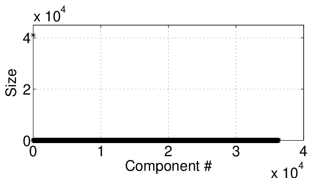
Table 1 shows the relevant statistics at the cut-off point for the two networks. Note that the cut-off point is attained at the expense of a relatively small number of high degree nodes ( for Epinions and for SlashDot). Moreover, the number of nodes in the is indeed roughly half of the overall order, albeit the is surely sparser in terms of edge density than the overall network ( vs. for Epinions and vs. for Slashdot). Fig. 7 (c-d) shows the sizes (in terms of nodes) of all the connected components for the respective graphs at the cut-off point. It is easy to see that other than the , the remaining components are of negligibly small orders. Recombining the non- components together (including the rich club) yields an interesting result. For the Epinions network, we obtain two sub-graphs of orders and respectively while for the Slashdot network we obtain exactly one sub-graph of order . This clearly demonstrates that our simple divide method, yields a roughly equal partitioning of the network — and thus comparable sub-problems — in terms of nodes. The pseudo-inverses of these sub-problems can now be computed in parallel. Albeit, as in the case of all tradeoffs, this equitable split comes at a price of roughly edges that violate the cut (c.f. Table 1). This yields an average cost for the two-stage process (c.f. §3). However, given the element-wise parallelizability of our method, we obtain the pseudo-inverses in acceptable times of roughly minutes for the Epinions and minutes for the SlashDot networks.
6 Related Work
The applications of the Moore-Penrose pseudo-inverse and the sub-matrix inverses of the Laplacian for a graph are multifarious. We discuss a few instances here in summary. As alluded to earlier, is used to compute effective resistance distances between the nodes of a graph [33] as well as the one way hitting and commute times in random walks between node pairs in a graph. All these distances serve as measures of multi-hop dissimilarity between nodes and find applications in several graph mining contexts [14, 28]. Moreover, for every connected undirected graph there is an analogous reversible Markov chain, finds use in the computation of relevant metrics (such as hitting time, cover time and mixing rates).
is a gram-matrix. Its eigen decomposition yields an Euclidean embedding of the graph whereby each node in the graph is represented as a point in that space. The general term represents the inner product of the respective position vectors for the nodes and and thus is a valid kernel for a graph. This geometric interpretation has been used in collaborative recommendation systems [28, 27, 29].
In [15, 16] the elements of have been given an elegant topological interpretation in terms of the dense spanning rooted forests of the graph. Namely, the general term represents the number of spanning rooted forests of the graph with exactly two trees in which the pair is in the same tree, rooted at (or by symmetry). Combining the geometric interpretation from [28, 27, 29] and the topological interpretation from [15, 16], the diagonal elements of have been used as centrality indices for the nodes of a complex network in [46]. This centrality index, called topological centrality, reflects both the overall position as well as the overall connectedness of nodes in the network. Consequently, it is a measure of the robustness of node to random multiple failures in the network. By extension, , also called the Kirchhoff index of a graph [33, 55], is a global structural descriptor for the graph on a whole. This index is quite popular in the field of mathematical chemistry and is used to measure overall molecular strength [42, 43, 44, 45].
7 Conclusion and Future Work
In this work, we presented a divide-and-conquer based approach for computing the Moore-Penrose pseudo-inverse of the Laplacian () for a simple, connected, undirected graph. Our method relies on an elegant interplay between the elements of and the pairwise effective resistance distances in the graph. Exploiting this relationship, we derived closed form solutions that enable us to compute in an incremental fashion. We also extended these results to analogous cases for structural regress. Using dynamic networks and online social networks as examples, we demonstrated the efficacy of our method for computing the pseudo-inverse relatively faster than the standard methods. The insights from our work open up several interesting questions for future research. First and foremost, similar explorations can be done for the case of directed graphs (asymmetric relationships), where analogous distance functions — such as the expected commute time in random walks — are defined, albeit the Laplacians (more than one kind in literature) are no longer symmetric [10]. Secondly, matrix-distance interplays of the kind exploited in this work, also exist for a general case of the so called forest matrix and its distance counterpart the forest distance [2, 15], both for undirected and directed graphs. he results presented here should find natural extensions to the forest matrix and the forest metric, at least for the undirected case. Finally, our closed forms can be used in conjunction with several interesting approaches for sparse inverse computations [13], to further expedite the pseudo-inverse computation for large generalized graphs. All these motivate ample scope for future work.
| Operation | ||
|---|---|---|
| First Join | ||
| Edge firing | ||
| Non-bridge delete | ||
| Bridge delete |
8 Acknowledgment
This research was supported in part by DTRA grant HDTRA1-09-1-0050 and NSF grants CNS-0905037, CNS-1017647, CNS-1017092 and IIS-0916750.
9 Appendix
9.1 Proof of Theorem 1
Given, , we note that and , where and are vectors of length containing all and respectively. From [10], we have:
| (18) |
where is the identity matrix of dimension and are vectors of all of length . Expanding we obtain the following scalar form:
| (19) |
9.2 Proof of Lemma 1
Given, is symmetric and doubly centered and , we have:
Rearranging terms, we get:
| (20) |
Substituting , in the expression above, we obtain the proof.
9.3 Proof of Corollary 1
Given, a star with node as root and nodes as leaves, we have:
| (21) |
Therefore,
Also,
Substituting for these values in Lemma 1, and noting that is doubly-centered, we obtain the proof.
9.4 Proof of Corollary 2
Given a clique of order , [9]. Therefore,
Also,
Substituting in Lemma 1, we obtain: and, from the fact that is doubly-centered, .
9.5 Proof of Theorem 2
We present the proofs for the following two cases: (a) and, (b) and . It is obvious that the other two cases, viz. (c) and (d) and , follow from symmetry. But first we must express as a function of , which is useful to us in both cases.
Lemma 2
For two disjoint simple, connected, undirected graphs and , let be the graph resulting from the first join between and by means of introducing an edge . Then,
| (22) |
9.5.1 Proof of Lemma 2
For an arbitrary node :
Therefore,
Summing up over all nodes :
By symmetry,
Therefore,
Now, substituting , we obtain the result.
9.5.2 Rest of the Proof of Theorem 2
Case a:
From Lemma 1, we have:
| (23) |
For the triangle inequality in the above:
By symmetry,
Finally, for the last of the three terms:
Summing the three individual
terms along with the value of from (22)
and substituting the result in (23), we obtain the proof.
Case b: and
Once again,
| (24) |
For the triangle inequality in the above:
Similarly,
And finally,
Summing the three individual terms along with the value of from (22) and substituting the result in (24), we obtain the proof.
9.6 Proof of Theorem 3
We prove Theorem 3 in two steps. First, in the following lemma, we provide a general result for a perturbation of a positive semi-definite matrix, which is then used to prove the overall theorem.
Lemma 3
Given is a symmetric, positive semi-definite matrix and a perturbation matrix, such that has an inverse where , and , the following holds:
| (25) |
9.6.1 Proof of Lemma 3:
Observe that the positive semi-definiteness of guarantees that has an inverse.
Let . Therefore,
From this identity, and the symmetry of , it follows easily that satisfies the four conditions required for a Moore-Penrose pseudo-inverse.
9.6.2 Rest of the Proof of Theorem 3
Note that the firing of the edge in to obtain , results in the following scalar relationships between the Laplacians of the two graphs:
| (26) |
For ease of exposition, we permute the rows and columns in and in such a way that and . The above perturbations can then be rewritten as:
| (27) |
is therefore a sum of , a real, symmetric, positive semi-definite matrix, and a perturbation matrix, referred to henceforth as . It is easy to see that for a simple, connected, undirected graph , satisfies all the preconditions in Lemma 3. Substituting , and , in Lemma 3, we get:
| (28) |
All that remains now is to obtain the scalar form for the term: . Note:
| (29) |
Similarly,
| (30) |
Or,
| (31) |
where , which yields:
| (32) |
Multiplying on the left and right sides of the above with and respectively, the following scalar form is obtained:
| (33) |
Substituting and back into the equation above, we obtain the proof.
9.7 Proof of Corollary 3
Noting and substituting into the result of Theorem 3, we obtain the proof.
9.8 Proof of Theorem 4
Deleting a non-bridge edge from to obtain , results in the following scalar relationships between the Laplacians of the two graphs:
| (34) |
Once again, for convenience, we rearrange the rows and columns of and in such a way that and . Thus,
| (35) |
The rest of the proof follows as in the proof of Theorem 3, with the following modification. Substituting , and , in Lemma 3, we get:
| (36) |
which yields the following scalar form:
| (37) |
Substituting and back into the equation above, we obtain the proof.
9.9 Proof of Corollary 4
Noting and substituting into the result of Theorem 4, we obtain the proof.
9.10 Proof of Theorem 5
We present the proof for the case: as the other case follows by symmetry. Once again, we need a lemma to determine in terms of the elements of .
Lemma 4
Let be a simple, connected, unweighted graph with a bridge edge which upon deletion produces two disjoint simple graphs and . Then,
| (38) |
9.10.1 Proof of Lemma 4
The proof follows simply by observing , and substituting values in terms of the elements of .
9.10.2 Rest of the Proof of Theorem 5
Follows similarly from the triangle inequality in Lemma 1, by confining to node pairs , and then substituting the result of Lemma 4 and other relevant effective resistance values in terms of .
References
- [1] http://snap.stanford.edu/data/.
- [2] R. Agaev and P. Chebotarev. The matrix of maximum out forests of a digraph and its applications. Automation and Remote Control, 61(9):1424–1450, 2000.
- [3] R. Albert, H. Jeong, and A. L. Barabási. Error and attack tolerance of complex networks. Nature, 406(6794):378–382, 2000.
- [4] N. Alon. Eigenvalues and expanders. Combinatorica, 6(2):83–96, 1986.
- [5] C. J. Alpert and A. B. Kahng. Recent directions in netlist partitioning: A survey. INTEGRATION(the VLSI journal).
- [6] E. Amir, R. Krauthgamer, and S. Rao. Constant factor approximation of vertex-cuts in planar graphs. In Proceedings of the 35th annual ACM symposium on Theory of computing, STOC ’03, pages 90–99, New York, NY, USA, 2003. ACM.
- [7] A. L. Barabási and R. Albert. Emergence of scaling in random networks. Science, 286(5439):509–512, 1999.
- [8] A. Ben-Israel and T. Greville. Generalized Inverses: Theory and Applications, edition. Springer-Verlag, 2003.
- [9] N. Biggs. Algebraic Graph Theory. Cambridge University Press, 1993.
- [10] D. Boley, G. Ranjan, and Z.-L. Zhang. Commute times for a directed graph using an asymmetric laplacian. Linear Algebra and its Applications, 435(2):224–242, 2011.
- [11] B. Bollobás. Random Graphs. Cambridge University Press, 2001.
- [12] M. Brand. A random walks perspective on maximizing satisfaction and profit. In Proc. 2005 SIAM Int’l Conf. Data Mining, 2005.
- [13] Y. E. Campbell and T. A. Davis. Computing the sparse inverse subset: An inverse multifrontal approach. Tech. report TR-95-021, Univ. of Florida, Gainesville, 1995.
- [14] A. K. Chandra, P. Raghavan, W. L. Ruzzo, R. Smolensky, and P. Tiwari. The electrical resistance of a graph captures its commute and cover times. In Proc. of Annual ACM Symposium on Theory of Computing, pages 574–586, 1989.
- [15] P. Chebotarev and E. Shamis. The matrix-forest theorem and measuring relations in small social groups. Automation and Remote Control, 58(9):1505–1514, 1997.
- [16] P. Chebotarev and E. Shamis. On proximity measures for graph vertices. Automation and Remote Control, 59(10):1443–1459, 1998.
- [17] J. Chlebikova. Approximating the maximally balanced connected partitions problem in graphs. Information Processing Letters, 60:225–230, 1996.
- [18] F. R. Chung. Spectral Graph Theory. Am. Math. Soc., 1997.
- [19] W. E. Donath and A. J. Hoffman. Lower bounds for the partitioning of graphs. IBM J. of Res. and Dev., 17:410–425, 1973.
- [20] P. G. Doyle and J. L. Snell. Random Walks and Electric Networks. The Math. Assoc. of America, 1984.
- [21] J. Edmonds and R. M. Karp. Theoretical improvements in algorithmic efficiency for network flow problems. Journal of the ACM, 19(2):248–264, 1972.
- [22] M. Faloutsos, P. Faloutsos, and C. Faloutsos. On power-law relationships of the internet topology. In Proc. of the ACM SIGCOMM, pages 251–262, 1999.
- [23] I. J. Farkas, I. Derényi, A. L. Barabási, and T. Vicsek. Spectra of real world graphs: Beyond the semicircle law. Physical Review E, 64(2), 2001.
- [24] M. Fiedler. Algebraic connectivity of graphs. Czechoslovak Math. J., 23:298–305, 1973.
- [25] M. Fiedler. A property of eigenvectors of nonnegative symmetric matrices and its applications to graph theory. Czechoslovak Math. J., 25(100):619–633, 1975.
- [26] L. R. Ford and D. R. Fulkerson. Maximal flow through a network. Canadian Journal of Mathematics, 8:399–404, 1956.
- [27] F. Fouss, A. Pirotte, J. M. Renders, and M. Saerens. A novel way of computing similarities between nodes of a graph, with application to collaborative recommendation. In Proc. 2005 IEEE/WIC/ACM Int’l Joint Conf. Web Intelligence, pages 550–556, 2005.
- [28] F. Fouss, A. Pirotte, J. M. Renders, and M. Saerens. Random-walk computation of similarities between nodes of a graph with application to collaborative recommendation. IEEE Transactions on Knowledge and Data Engineering, 19, 2007.
- [29] F. Fouss, L. Yen, A. Pirotte, and M. Saerens. An experimental investigation of graph kernels on a collaborative recommendation task. In Proc. of the 6th International Conference on Data Mining, 2006.
- [30] F. Gobel and A. Jagers. Random walks on graphs. Stochastic Processes and Their Applications, 2:311–336, 1974.
- [31] D. Isaacson and R. Madsen. Markov Chains Theory and Applications. John Wiley and Sons, 1976.
- [32] S. J. Kirkland, M. Neumann, and B. L. Shader. Distances in weighted trees and group inverse of laplacian matrices. SIAM Journal of Matrix Anal. Appl., 18:827–841, 1997.
- [33] D. J. Klein and M. Randić. Resistance distance. J. Math. Chemistry, 12:81–95, 1993.
- [34] U. V. Luxburg. A tutorial on spectral clustering. Statistics and Computing, 17(4):395–416, December 2007. Max Planck Institute for Biological Cybernetics. Technical Report No. TR-149.
- [35] U. V. Luxburg, A. Radl, and M. Hein. Getting lost in space: Large sample analysis of the commute distance. NIPS, 2010.
- [36] C. D. Meyer. Generalized inversion of modified matrices. SIAM Journal on Applied Mathematics, 24(3):315–323, 1973.
- [37] B. Mohar. The Laplace spectrum of graphs. In Graph Theory, Combinatorics, and Applications, volume 2, pages 871–898. Wiley, 1991.
- [38] B. Mohar. Laplace eigenvalues of graphs - a survey. Discrete Math., 109:171–183, 1992.
- [39] B. Mohar. Some applications of Laplace eigenvalues of graphs. In Graph Symmetry: Algebraic Methods and Applications, volume NATO ASI Ser C 497, pages 225–275. Kluwer, 1997.
- [40] M. E. J. Newman. A measure of betweenness centrality based on random walks. Social Networks, 27(1):39–54, 2005.
- [41] A. Nilli. On the second eigenvalue of a graph. Discrete Mathematics, 91(2):207–210, 1991.
- [42] J. L. Palacios. Closed-form formulas for kirchhoff index. Intl. Journal of Quantum Chemistry, 81:135–140, 2001.
- [43] J. L. Palacios. On the kirchhoff index of regular graphs. Intl. Journal of Quantum Chemistry, 110:1307–1309, 2001.
- [44] J. L. Palacios. Resistance distance in graphs and random walks. Intl. Journal of Quantum Chemistry, 81:29–33, 2001.
- [45] J. L. Palacios and J. M. Renom. Bounds for the kirchhoff index of regular graphs via the spectra of their random walks. Intl. Journal of Quantum Chemistry, 110:1637–1641, 2001.
- [46] G. Ranjan and Z.-L. Zhang. Geometry of complex networks and topological centrality. arXiv:1107.0989, 2011.
- [47] M. Saerens, F. Fouss, L. Yen, and P. Dupont. The principal components analysis of a graph, and its relationships to spectral clustering. In Proc. 15th European Conf. Machine Learning (ECML ’04), pages 371–383, 2004.
- [48] B. Sarwar, G. Karypis, J. Konstan, , and J. Riedl. Recommender systems for large-scale e-commerce: Scalable neighborhood formation using clustering. In Proc. Fifth Int’l Conf. Computer and Information Technology, 2002.
- [49] A. Sen, P. Ghosh, B. Yang, and V. Vittal. A new min-cut problem with application to electric power network partitioning. European Transactions on Electrical Power, 2008.
- [50] J. Shi and J. Malik. Normalised cuts and image segmentation. IEEE Trans. Pattern Analysis and Machine Intelligence, 22(8):888–905, 1997.
- [51] B. Tadić and V. Priezzhev. Voltage distribution in growing conduction networks. European Physical Journal B, 30:143–146, 2002.
- [52] P. Tetali. Random walks and effective resistance of networks. Journal of Theoretical Probability, pages 101–109, 1991.
- [53] S. Tiptipakorn. A spectral bisection partitioning method for electric power network applications. PhD dissertation, Dept. of Elec. and Comp. Engineering, Univ. of Wisconsin, 2001.
- [54] D. J. Watts and S. H. Strogatz. Collective dynamics of ‘small-world’ networks. Nature, 393:440–442, 1998.
- [55] W. Xiao and I. Gutman. Resistance distance and laplacian spectrum. Theoretical Chemistry Accounts, 110:284–289, 2003.