The Deformed Consensus Protocol
Extended Version

Fabio Morbidi Email: fabio.morbidi@inria.fr

Abstract

This paper studies a generalization of the standard continuous-time consensus protocol, obtained by replacing the Laplacian matrix of the communication graph with the so-called deformed Laplacian. The deformed Laplacian is a second-degree matrix polynomial in the real variable $s$ which reduces to the standard Laplacian for $s$ equal to unity. The stability properties of the ensuing deformed consensus protocol are studied in terms of parameter $s$ for some special families of undirected and directed graphs, and for arbitrary graph topologies by leveraging the spectral theory of quadratic eigenvalue problems. Examples and simulation results are provided to illustrate our theoretical findings.

keywords

Multi-agent systems; consensus algorithms; cooperative control; sensor networks; autonomous mobile robots

^†^†thanks: [^†^†address: Institute for Design and Control of Mechatronical Systems, Johannes Kepler University, Altenbergerstraße 69, 4040 Linz, Austria

footnoteinfo]The author is currently with the Networked Controlled System (NeCS) team, Inria Grenoble Rhône-Alpes, 655 Avenue de l’Europe, Montbonnot, 38334 Saint Ismier cedex, France, telephone ( $+$ 04) 76 61 53 22. The author gratefully acknowledges the sponsoring of this work by the COMET K2 center “Austrian Center of Competence in Mechatronics” (ACCM).

1 Introduction

In the last decade we have witnessed a spurt of interest in multi-agent systems research, in the control, telecommunication and robotics communities [BulloCoMa_book09, MesbahiEg_book10, Zampieri_IFAC08, Springer_Handbook08_ch41]. Distributed control and consensus problems [OlfatiFaMu_IEEE07, RenBeAt_CSM07], have had a large share in this research activity. Consensus theory originated from the work of Tsitsiklis [Tsitsiklis_PhD84], Jadbabaie et al. [JadbabaieJiMo_TAC03] and Olfati-Saber et al. [OlfatiSaberMu_TAC04], in which the consensus problem was formulated for the first time in system-theoretical terms. A very rich literature emanated from these seminal contributions in recent years. In particular, numerous extensions to the prototypal consensus protocol in [OlfatiSaberMu_TAC04] have been proposed: among them, we limit ourselves to mention here the cases of time-varying network topology [Moreau_TAC05, RenBe_TAC05], of networks with delayed [OlfatiSaberMu_TAC04] or quantized/noisy communication and link failure [FrascaCaFaZa_IJRNC09, KarMo_TSP09], of random networks [PorfiriSt_TAC07, TahbazJa_TAC08, FagnaniZa_JSAC08], of networks with antagonistic interactions [Altafini_PLOSONE12, Altafini_TAC13], of distributed average tracking [SpanosOlMu_IFAC05, YangFrLy_TAC08, ChenCaRe_TAC12], of finite-time consensus [WangXi_TAC10, Kibangou_ACC12], of logical [FagioliniViBi_CDC08] and nonlinear agreement [BausoGiPe_SCL06, Cortes_AUTO08], and of consensus over finite fields [PasqualettiBoBu_AUTO13].
This paper follows this active line of research and proposes an original extension to the basic continuous-time consensus protocol in [OlfatiSaberMu_TAC04], that exhibits a rich variety of behaviors and whose flexibility makes it ideal for a broad range of mobile robotic applications (e.g., for clustering, or for containment and formation control). The new protocol, termed deformed consensus protocol, relies on the so-called deformed Laplacian matrix, a second-degree matrix polynomial in the real variable $s$ , which extends the standard Laplacian matrix and reduces to it for $s$ equal to unity: the deformed Laplacian is indeed an instance of a more general theory of deformed differential operators developed in mathematical physics in the last three decades, cf. [HislopSi_book96, Ch. 18]. Parameter $s$ has a dramatic effect on the stability properties of the deformed consensus protocol, and it can be potentially used by a supervisor to dynamically modify the behavior of the network and trigger different desired agents’ responses according to time-varying external events. The stability properties of the proposed protocol are studied in terms of parameter $s$ for some special families of undirected and directed graphs for which the eigenvalues and eigenvectors of the negated deformed Laplacian can be computed in closed form. In the case of directed graphs, it is shown that differently from the standard consensus algorithm, for some values of $s$ the states of the deformed consensus protocol may also experience stable steady-state oscillations. Our analysis is extended to arbitrary graph topologies by exploiting the spectral theory of quadratic eigenvalue problems [TisseurMe_SIAM01]. The discrete-time version of our consensus protocol, that involves the so-called deformed Perron matrix, is also briefly discussed.
Beside the aforementioned promising applications, we believe that the study of the proposed protocol is of value for shedding new light on known results [OlfatiSaberMu_TAC04, RenBe_TAC05], and for gaining a more general perspective on consensus algorithms.
A preliminary version of this paper appeared in [Morbidi_CDC12], compared to which we present here several new theoretical results as well as more extensive numerical simulations.
The rest of the article is organized as follows. In Sect. 2 we review some relevant notions of algebraic graph theory. The main theoretical results of the paper are presented in Sect. 3. In Sect. 4, two possible extensions of our results are discussed. Finally, in Sect. 5, the theory is illustrated via numerical simulations, and in Sect. 6 the main contributions of the paper are summarized and possible future research directions are outlined.

2 Preliminaries

In this section, we briefly recall some basic notions of algebraic graph theory that will be used through the paper. Let $\mathcal{G}=(V,\,E)$ be an undirected graph¹¹ 1 All graphs in this paper are finite, and with no self-loops and multiple edges. where $V=\{1,\ldots,n\}$ is the set of vertices, and $E$ is the set of edges [GodsilRo_book01].

Definition 1 (Adjacency matrix ${\mathbf{A}}$ )

The adjacency matrix ${\mathbf{A}}=[a_{ij}]$ of graph $\mathcal{G}$ is an $n\times n$ matrix defined as,

a_{ij}\,=\,\left\{\begin{array}[]{ll}1&\text{if}\;\;\{i,\,j\}\in E,\\ 0&\text{otherwise}.\end{array}\right.\vskip-12.80365pt

$\diamond$

Definition 2 (Laplacian matrix ${\mathbf{L}}$ )

The Laplacian matrix of graph $\mathcal{G}$ is an $n\times n$ matrix defined as,

{\mathbf{L}}\,=\,{\mathbf{D}}-{\mathbf{A}},

where ${\mathbf{D}}=\text{diag}({\mathbf{A}}\mathds{1})$ is the degree matrix²² 2 $\text{diag}({\mathbf{b}})$ is a diagonal matrix with the elements of the vector ${\mathbf{b}}\in\mathop{{\rm I}\mskip-4.0mu{\rm R}}\nolimits^{n}$ put on its main diagonal. and $\mathds{1}=\mathds{1}_{n}$ is a column vector of $n$ ones. $\diamond$

Note that the Laplacian ${\mathbf{L}}$ is a symmetric positive semidefinite matrix [Mohar_GRCA91].

Property 1 (Spectral properties of ${\mathbf{L}}$ )

Let $\lambda_{1}({\mathbf{L}})\leq\lambda_{2}({\mathbf{L}})\leq\ldots\leq\lambda_{n}({\mathbf{L}})$ be the ordered eigenvalues of the Laplacian ${\mathbf{L}}$ . Then, we have that [Abreu_LAA07]:

1.

$\lambda_{1}({\mathbf{L}})=0$ with corresponding eigenvector $\mathds{1}$ . The algebraic multiplicity of $\lambda_{1}({\mathbf{L}})$ is equal to the number of connected components in $\mathcal{G}$ .
2.

$\lambda_{2}({\mathbf{L}})>0$ if and only if the graph $\mathcal{G}$ is connected. $\lambda_{2}({\mathbf{L}})$ is called the algebraic connectivity or Fiedler value of the graph $\mathcal{G}$ . $\diamond$

Definition 3 (Bipartite graph)

A graph $\mathcal{G}$ is called bipartite if its vertex set $V$ can be divided into two disjoint sets $V_{1}$ and $V_{2}$ , such that every edge connects a vertex in $V_{1}$ to one in $V_{2}$ . Equivalently, we have that a graph is bipartite if and only if it does not contain cycles of odd length. $\diamond$

Definition 4 (Signless Laplacian matrix ${\mathbf{Q}}$ )

The signless Laplacian matrix of graph $\mathcal{G}$ is defined as [CvetkovicRoSi_LAA07]

{\mathbf{Q}}\,=\,{\mathbf{D}}+{\mathbf{A}}.\vskip-18.49411pt

$\diamond$

Note that as ${\mathbf{L}}$ , the signless Laplacian ${\mathbf{Q}}$ is a symmetric positive semidefinite matrix (but it is not necessarily singular [BrouwerHa_book12]). Indeed, ${\mathbf{Q}}\,=\,{\mathbf{R}}{\mathbf{R}}^{T}$ where ${\mathbf{R}}$ is the vertex-edge incidence matrix³³ 3 The vertex-edge incidence matrix of a graph $\mathcal{G}$ is the 0-1 matrix ${\mathbf{R}}=[r_{ik}]$ , with rows indexed by the vertices and column indexed by the edges, where $r_{ik}=1$ when vertex $i$ is an endpoint of edge $k$ . of $\mathcal{G}$ .

Property 2 (Spectral properties of ${\mathbf{Q}}$ )

The signless Laplacian ${\mathbf{Q}}$ has the following spectral properties:

1.

If $\lambda_{1}({\mathbf{L}})\leq\lambda_{2}({\mathbf{L}})\leq\ldots\leq\lambda_{n}({\mathbf{L}})$ and $\lambda_{1}({\mathbf{Q}})\geq\lambda_{2}({\mathbf{Q}})\geq\ldots\geq\lambda_{n}({\mathbf{Q}})$ are the ordered eigenvalues of the Laplacian and signless Laplacian, respectively, then we have that [CvetkovicRoSi_LAA07]:

$\lambda_{n}({\mathbf{L}})\,\leq\,\lambda_{1}({\mathbf{Q}}).$

Moreover, if $n\geq 2$ we have that

$\lambda_{2}({\mathbf{L}})\,\leq\,\lambda_{2}({\mathbf{Q}})+2,\vskip 1.42271pt$

with equality if and only if $\mathcal{G}$ is the complete graph $K_{n}$ [CvetkovicSi_PIMB09, Th. 3.5].
2.

If $\mathcal{G}$ is a connected graph with $n$ vertices and $m$ edges, then

$\lambda_{1}({\mathbf{Q}})\leq\frac{2\,m}{n-1}+n-2,$

with equality if and only if $\mathcal{G}$ is the star graph $K_{1,\,n-1}$ or the complete graph $K_{n}$ [CvetkovicSi_AADM10, Th. 1].
3.

We have that

$\textup{trace}({\mathbf{L}})\,=\,\textup{trace}({\mathbf{Q}})\,=\ 2\,|E|,$

where $|E|$ denotes the cardinality of the edge set $E$ [BrouwerHa_book12].
4.

A graph $\mathcal{G}$ is regular (i.e., each vertex of $\mathcal{G}$ has the same degree) if and only if its signless Laplacian has an eigenvector whose components are all ones [CvetkovicSi_PIMB09, Prop. 2.1].
5.

If $\mathcal{G}$ is a regular graph of degree $\kappa$ (i.e., each vertex of $\mathcal{G}$ has the same degree $\kappa\leq n-1$ ), then,

$p_{{\mathbf{L}}}(\lambda)=(-1)^{n}\,p_{{\mathbf{Q}}}(2\kappa-\lambda),$

where $p_{{\mathbf{L}}}(\lambda)$ denotes the characteristic polynomial of the Laplacian ${\mathbf{L}}$ . If $\mathcal{G}$ is a bipartite graph, then [CvetkovicRoSi_LAA07, Prop. 2.3],

$p_{{\mathbf{L}}}(\lambda)\,=\,p_{{\mathbf{Q}}}(\lambda).$
6.

The least eigenvalue of ${\mathbf{Q}}$ of a connected graph is equal to $0$ if and only if the graph is bipartite. In this case, $0$ is a simple eigenvalue [CvetkovicRoSi_LAA07, Prop. 2.1].
7.

In any graph, the multiplicity of the eigenvalue 0 of ${\mathbf{Q}}$ is equal to the number of bipartite components of the graph $\mathcal{G}$ [BrouwerHa_book12, Prop. 1.3.9].
8.

Let $\mathcal{G}$ be a regular bipartite graph of degree $\kappa$ . Then the spectrum of ${\mathbf{Q}}$ is symmetric with respect to the point $\kappa$ [CvetkovicSi_PIMB09, Prop. 2.2]. $\diamond$

Let $\mathcal{D}=(V,\,E)$ be a directed graph (or digraph, for short) where $V=\{1,\ldots,n\}$ is the set of vertices and $E\subseteq V\!\times V$ is the set of edges. In the case of directed graphs, we can define the adjacency and degree matrix, as,

a_{ij}\,=\,\left\{\begin{array}[]{ll}1&\text{if}\;\;(j,\,i)\in E,\\ 0&\text{otherwise},\end{array}\right.

and ${\mathbf{D}}=\text{diag}(d_{\text{in}}(1),\ldots,d_{\text{in}}(n))$ , where $d_{\textup{in}}(i)$ denotes the in-degree of vertex $i$ with $i\in\{1,\ldots,n\}$ (i.e., the number of directed edges pointing at vertex $i$ ). With these definitions in hand, the in-degree Laplacian ${\mathbf{L}}(\mathcal{D})$ and in-degree signless Laplacian ${\mathbf{Q}}(\mathcal{D})$ of $\mathcal{D}$ , can be defined as in the undirected case⁴⁴ 4 “Out-degree” versions of ${\mathbf{L}}(\mathcal{D})$ and ${\mathbf{Q}}(\mathcal{D})$ can be similarly introduced, but they will not be considered in this paper.. Note that ${\mathbf{L}}(\mathcal{D})$ and ${\mathbf{Q}}(\mathcal{D})$ are nonsymmetric matrices, and that all the eigenvalues of ${\mathbf{L}}(\mathcal{D})$ have non-negative real parts (this can be easily proved using Geršgorin’s disk theorem [OlfatiFaMu_IEEE07]).

The following definitions will be used in Sect. 4.2.

Definition 5 (Bipartite digraph)

A digraph $\mathcal{D}=(V,\,E)$ is called bipartite if its vertex set $V$ can be divided into two disjoint sets $V_{1}$ and $V_{2}$ , such that $E\cap(V_{1}\times V_{1})=\emptyset$ and $E\cap(V_{2}\times V_{2})=\emptyset$ , where $\emptyset$ denotes the empty set. $\diamond$

Definition 6 (Rooted out-branching)

A digraph $\mathcal{D}=(V,\,E)$ is a rooted out-branching if [MesbahiEg_book10]:

1.

It does not contain a directed cycle;
2.

It has a vertex $v_{\textup{R}}$ (root) such that for every other vertex $v\in V$ , there is a directed path from $v_{\textup{R}}$ to $v$ . $\diamond$

Definition 7 (Strongly connected digraph)

A digraph is strongly connected if, between every pair of distinct vertices, there is a directed path. $\diamond$

Definition 8 (Weakly connected digraph)

A digraph is weakly connected if its disoriented version (i.e. the graph obtained by replacing all its directed edges with undirected ones), is connected. $\diamond$

Definition 9 (Balanced digraph)

A digraph is called balanced if, for every vertex, the in-degree and out-degree are equal, i.e., $d_{\textup{in}}(i)\,=\,d_{\textup{out}}(i)$ , for all $i\in\{1,\ldots,n\}$ . $\diamond$

3 Deformed consensus protocol

3.1 Problem formulation

It is well-known [OlfatiSaberMu_TAC04], that if the static undirected communication graph $\mathcal{G}$ is connected, each component of the state vector ${\mathbf{x}}\triangleq[x_{1},\ldots,x_{n}]^{T}\in\mathop{{\rm I}\mskip-4.0mu{\rm R}}\nolimits^{n}$ of the linear time-invariant system,

\dot{{\mathbf{x}}}(t)\,=\,-{\mathbf{L}}\,{\mathbf{x}}(t),

(1)

asymptotically converges to the average of the initial states $x_{1}(0),\ldots,x_{n}(0)$ ,

\lim_{t\rightarrow\infty}\;x_{i}(t)\,=\,\frac{1}{n}\,\sum_{i\,=\,1}^{n}\,x_{i}(0)\,=\,\frac{1}{n}\;{\mathbf{x}}_{0}^{T}\,\mathds{1},

where ${\mathbf{x}}_{0}\triangleq[x_{1}(0),\,\ldots,\,x_{n}(0)]^{T}$ , i.e., average consensus is achieved. The converge rate of the consensus protocol (1) is dictated by the algebraic connectivity $\lambda_{2}({\mathbf{L}})$ .
Let us now consider the following generalization of the Laplacian ${\mathbf{L}}$ .

Definition 10 (Deformed Laplacian $\boldsymbol{\Delta}(s)$ )

The deformed Laplacian of the graph $\mathcal{G}$ is an $n\times n$ matrix defined as,

\boldsymbol{\Delta}(s)\,=\,({\mathbf{D}}-{\mathbf{I}}_{n})\,s^{2}\,-\,{\mathbf{A}}\,s\,+\,{\mathbf{I}}_{n},

where ${\mathbf{I}}_{n}$ is the $n\times n$ identity matrix, and $s$ is a real parameter. $\diamond$

Note that $\boldsymbol{\Delta}(s)$ is a symmetric matrix (but not positive semidefinite as ${\mathbf{L}}$ , in general), and that:

\boldsymbol{\Delta}(1)={\mathbf{L}},\quad\;\boldsymbol{\Delta}(-1)={\mathbf{Q}}.

Since $\boldsymbol{\Delta}(0)={\mathbf{I}}_{n}$ , the deformed Laplacian is a comonic polynomial matrix [GohbergLaRo_Book09, Sect. 7.2].

The following lemma shows an interesting connection between the spectrum of the deformed Laplacian and the spectrum of the corresponding adjacency matrix, for regular graphs.

Lemma 1

Let $\mathcal{G}$ be a regular graph of degree $\kappa$ . Then,

\lambda_{i}(\boldsymbol{\Delta}(s))\,=\,(\kappa-1)\,s^{2}-\lambda_{i}({\mathbf{A}})\,s+1,\;\;\,i\in\{1,\ldots,n\}.\vskip-5.69046pt

$\blacksquare$

Inspired by (1), we will study the stability properties of the following linear system,

\dot{{\mathbf{x}}}(t)=-\boldsymbol{\Delta}(s)\,{\mathbf{x}}(t),

(2)

in terms of the real parameter $s$ , assuming that the graph $\mathcal{G}$ is connected. We will refer to (2), as the deformed consensus protocol.

Refer to caption — Figure 1: *Illustrative example*: The 6 agents rendezvous at the origin while avoiding the two obstacles (gray rectangles): this is made possible by switching $s$ from $-1$ to $0$ (the initial position of the vehicles is marked with a circle and the final position with a diamond).

Remark 1

Note that parameter $s$ in the deformed Laplacian $\boldsymbol{\Delta}(s)$ can be regarded as a control input and it can be exploited to dynamically modify the behavior of system (2). This may be useful when the vertices of the graph are mobile robots and a human supervisor is interested in changing the collective behavior of the team over time, cf. [MilutinovicLi_TRO06], e.g., by switching from a marginally- to an asymptotically-stable equilibrium point of system (2), or between two marginally-stable equilibria. The former case is illustrated in the example in Fig. 1, where the communication graph is the path graph $P_{6}$ : in order to make the 6 single-integrator agents rendezvous at the origin while avoiding the two gray obstacles, the supervisor can initially set $s=-1$ and then switch to $s=0$ (cf. Prop. 1 in Sect. 3.2). $\diamond$

Note that since $\boldsymbol{\Delta}(1)={\mathbf{L}}$ , we will always achieve average consensus for $s=1$ . Moreover, since $\boldsymbol{\Delta}(s)$ is real symmetric, all the eigenvalues of $\boldsymbol{\Delta}(s)$ (which are nonlinear functions of $s$ ) are real, and the deformed Laplacian admits the spectral decomposition $\boldsymbol{\Delta}(s)={\mathbf{U}}(s)\boldsymbol{\Lambda}(s){\mathbf{U}}^{T}(s)$ , where ${\mathbf{U}}(s)=[{\mathbf{u}}_{1}(s)\;{\mathbf{u}}_{2}(s)\,\ldots\,{\mathbf{u}}_{n}(s)]$ $\in\mathop{{\rm I}\mskip-4.0mu{\rm R}}\nolimits^{n\times n}$ is the matrix consisting of normalized and mutually orthogonal eigenvectors of $\boldsymbol{\Delta}(s)$ and $\boldsymbol{\Lambda}(s)=\text{diag}(\lambda_{1}(\boldsymbol{\Delta}(s)),\ldots,\lambda_{n}(\boldsymbol{\Delta}(s)))$ . The solution of (2), can thus be written as,

{\mathbf{x}}(t)\,=\,\sum_{i=1}^{n}\,\exp(-\lambda_{i}(\boldsymbol{\Delta}(s))t)\,({\mathbf{u}}_{i}^{T}(s)\,{\mathbf{x}}_{0})\,{\mathbf{u}}_{i}(s).

(3)

In Sect. 3.2, we will focus on some special families of undirected graphs for which the eigenvalues and eigenvectors of $\boldsymbol{\Delta}(s)$ can be computed in closed form, and thus the stability properties of system (2) can be easily deduced from (3). In Sect. 3.3, we will address, instead, the more challenging case of undirected graphs with arbitrary topology. Finally, some extensions (the discrete-time case, and the case of directed communication networks), will be discussed in Sect. 4.

3.2 Stability conditions for special families of graphs

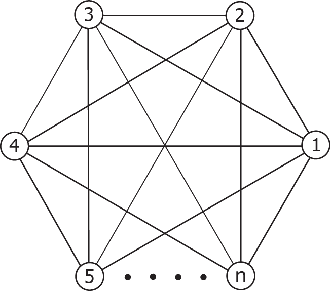
This section presents a sequence of nine propositions which provide stability conditions for system (2), in the case of path, cycle, full $m$ -ary tree, wheel, $m$ -cube (or hypercube), Petersen, complete, complete bipartite and star graphs (see Fig. 2 and refer to [GodsilRo_book01] for a precise definition of these graphs). In the following,

\mathds{k}\,\triangleq\,[-1,\,1,-1,\,1,\ldots,(-1)^{n-1},(-1)^{n}]^{T}\in\mathop{{\rm I}\mskip-4.0mu{\rm R}}\nolimits^{n},

$\mathds{J}_{m\times n}$ will denote the $m\times n$ ones matrix, ${\mathbf{0}}_{m\times n}$ the $m\times n$ zeros matrix, $\lfloor\cdot\rfloor$ the floor function which maps a real number to the largest previous integer, and $\lambda_{i}(s)$ will be used as a shorthand for $\lambda_{i}(-\boldsymbol{\Delta}(s))$ , $i\in\{1,\ldots,n\}$ .
In order to prove our first proposition, we need the following theorem [GolubLo_book96, Th. 8.5.1].

Theorem 1 (Sturm sequence property)

Consider the following $n\times n$ symmetric tridiagonal matrix,

{\mathbf{T}}\,=\left[\,\,\begin{matrix}a_{1}&b_{1}&&&\\ b_{1}&a_{2}&b_{2}&&\vskip-2.84544pt\\ &b_{2}&a_{3}&\!\!\ddots&\vskip-2.84544pt\\ &&\!\!\ddots&\ddots&b_{n-1}\\ &&&b_{n-1}&a_{n}\end{matrix}\,\right],

where $b_{j}\neq 0$ , $\forall\,j\in\{1,\ldots,n-1\}$ . Let ${\mathbf{T}}^{(r)}$ denote the leading $r\times r$ principal submatrix of ${\mathbf{T}}$ . Then, the number of negative eigenvalues of ${\mathbf{T}}$ is equal to the number of sign changes in the Sturm sequence:

1,\;\;\det({\mathbf{T}}^{(1)}),\;\det({\mathbf{T}}^{(2)}),\,\ldots,\;\det({\mathbf{T}}^{(n)}).

The result is still valid if zero determinants are encountered along the way, as long as we define a “sign change” to mean a transition from $+$ or 0 to $-$ , or from $-$ or 0 to $+$ , but not from $+$ or $-$ to 0. $\blacksquare$

Proposition 1 (Path graph $P_{n}$ )

For the path graph $P_{n}$ with $n\geq 2$ vertices (see Fig. 2(a)), we have that:

•

For $|s|<1$ , system (2) is asymptotically stable.
•

For $|s|>1$ , system (2) is unstable.
•

For $s=-1$ , system (2) is marginally stable. In this case, it is possible to identify two groups of $n/2$ vertices (if $n$ is even), or one group of $\lfloor n/2\rfloor$ vertices and one of $\lfloor n/2\rfloor+1$ vertices (if $n$ is odd). The states associated to the vertices in one group asymptotically converge to $\frac{1}{n}\,{\mathbf{x}}_{0}^{T}\mathds{k}$ and the states associated to the vertices in the other group converge to $-\frac{1}{n}\,{\mathbf{x}}_{0}^{T}\mathds{k}$ .

Proof: In this case, $-\boldsymbol{\Delta}(s)$ is a symmetric tridiagonal matrix,

-\boldsymbol{\Delta}(s)=\left[\,\begin{matrix}-1&s&&&\\ s&-(s^{2}+1)&s&&\vskip-3.41418pt\\ &&\ddots&&\vskip-1.13791pt\\ &&s&-(s^{2}+1)&s\\ &&&s&-1\end{matrix}\,\right].

The Sturm sequence of $-\boldsymbol{\Delta}(s)$ is given by

\begin{array}[]{ll}1,\;-1,\;1,\;-1,\;1,\,\ldots,\,-1,\;1,\;s^{2}-1,&\text{if}\;\,n\;\,\text{is odd},\\ 1,\;-1,\;1,\;-1,\;1,\,\ldots,\,1,\;-1,\;1-s^{2},&\text{if}\;\,n\;\,\text{is even}.\end{array}

Therefore by Theorem 1, if $|s|<1$ , $s\neq 0$ , all the eigenvalues of $-\boldsymbol{\Delta}(s)$ are strictly negative and system (2) is asymptotically stable. On the other hand, the Sturm sequence of $\boldsymbol{\Delta}(s)$ , for all $n$ , is given by $1,\;1,\ldots,\;1,\;1-s^{2}$ , from which we deduce that for $|s|>1$ , $\boldsymbol{\Delta}(s)$ has a negative eigenvalue, and hence system (2) is unstable. Since $\boldsymbol{\Delta}(0)={\mathbf{I}}_{n}$ , the system is asymptotically stable for $s=0$ . Finally, for $s=-1$ , system (2) is marginally stable and the unit-norm eigenvector associated to the zero eigenvalue of $-\boldsymbol{\Delta}(-1)$ is $\frac{1}{\sqrt{n}}\,\mathds{k}$ . $\blacksquare$

Proposition 2 (Cycle graph $C_{n}$ )

For the cycle graph $C_{n}$ with $n>2$ vertices (see Fig. 2(b)), we have that:

•
If $n$ is even:
- –
  
  For all $s\in\mathop{{\rm I}\mskip-4.0mu{\rm R}}\nolimits\setminus\{-1,\,1\}$ , system (2) is asymptotically stable.
- –
  
  For $s=-1$ , system (2) is marginally stable. In this case, the states associated to $n/2$ vertices asymptotically converge to $\frac{1}{n}\,{\mathbf{x}}_{0}^{T}\,\mathds{k}$ and the states associated to the other $n/2$ vertices converge to $-\frac{1}{n}\,{\mathbf{x}}_{0}^{T}\,\mathds{k}$ .
•

If $n$ is odd, system (2) is asymptotically stable for all $s\in\mathop{{\rm I}\mskip-4.0mu{\rm R}}\nolimits\setminus\{\,1\}$ .

Proof: In this case $-\boldsymbol{\Delta}(s)$ is a circulant matrix,

-\boldsymbol{\Delta}(s)=\textup{circ}[-(s^{2}+1),\,s,\,0,\,\ldots,\,0,\,s],

i.e., each subsequent row is simply the row above shifted one element to the right (and wrapped around, i.e., modulo $n$ ). The entire matrix is thus determined by the first row. It is well-known that circulant matrices are diagonalizable by the Fourier matrix ${\mathbf{F}}_{n}$ , given via,

{\mathbf{F}}^{\ast}_{n}=\frac{1}{\sqrt{n}}\left[\begin{array}[]{ccccc}1&1&1&\cdots&1\\ 1&\omega&\omega^{2}&\cdots&\omega^{n-1}\\ 1&\omega^{2}&\omega^{4}&\cdots&\omega^{2(n-1)}\\ \vdots&\vdots&\vdots&\ddots&\vdots\\ 1&\omega^{n-1}&\omega^{2(n-1)}&\cdots&\omega^{(n-1)(n-1)}\\ \end{array}\!\!\right],

where $\omega\triangleq e^{2\pi j/n}$ , $j=\sqrt{-1}$ , and ${\mathbf{F}}^{\ast}_{n}$ denotes the conjugate transpose of ${\mathbf{F}}_{n}$ , hence their eigenvalues can be computed in closed form. The eigenvalues of a general $n\times n$ circulant matrix ${\mathbf{C}}=\text{circ}[c_{1},\,c_{2},\ldots,\,c_{n}]$ , in fact, are given by:

\lambda_{i}({\mathbf{C}})=\rho_{{\mathbf{C}}}(\omega^{i-1}),\;\;i\in\{1,\ldots,\,n\},

(4)

where the polynomial $\rho_{{\mathbf{C}}}(\xi)=c_{n}\xi^{n-1}+\ldots+c_{3}\xi^{2}+c_{2}\xi+~c_{1}$ is called the circulant’s representer [Davis_book94, Th. 3.2.2]. By applying this result to matrix $-\boldsymbol{\Delta}(s)$ , for $i\in\{1,\ldots,\,n\}$ we have that,

\lambda_{i}(-\boldsymbol{\Delta}(s))\,=\,-\,s^{2}\,+\,2\,\cos\!\left(\frac{2\,\pi(i-1)}{n}\right)s\,-\,1.

(5)

Observe now that the coordinates of the vertex of the parabola (5) are

\left[\cos\!\left(\frac{2\pi(i-1)}{n}\right),\,-\sin^{2}\!\left(\frac{2\pi(i-1)}{n}\right)\!\right],\,i\in\{1,\,\ldots,\,n\}.

If $n$ is even, then $\lambda_{i}(-\boldsymbol{\Delta}(s))<0$ , $\forall\,s\in\mathop{{\rm I}\mskip-4.0mu{\rm R}}\nolimits$ and $\forall\,i\neq\{1,\,n/2\,+\,1\}$ . For $i=1$ , $\lambda_{1}(-\boldsymbol{\Delta}(s))\leq 0$ and $\lambda_{1}(-\boldsymbol{\Delta}(s))\,\,{=}\,\,0$ only for $s=1$ . For $i=n/2+1$ , $\lambda_{n/2\,+\,1}(-\boldsymbol{\Delta}(s))\leq 0$ and $\lambda_{n/2\,+\,1}(-\boldsymbol{\Delta}(s))=0$ only for $s=-1$ . The unit-norm eigenvector associated to $\lambda_{n/2\,+\,1}(-\boldsymbol{\Delta}(-1))$ is $\frac{1}{\sqrt{n}}\,\mathds{k}$ . On the other hand, if $n$ is odd, then $\lambda_{i}(-\boldsymbol{\Delta}(s))<0$ , $\forall\,s\in\mathop{{\rm I}\mskip-4.0mu{\rm R}}\nolimits$ and $\forall\,i\neq 1$ . For $i=1$ , $\lambda_{1}(-\boldsymbol{\Delta}(s))\leq 0$ and $\lambda_{1}(-\boldsymbol{\Delta}(s))=0$ only for $s=1$ . $\blacksquare$

Note that for the cycle graph $C_{n}$ ,

\det(-\boldsymbol{\Delta}(s))\,=\,(-1)^{n}\,(s^{2n}-2s^{n}+1),

and that the $2n$ roots of $\det(-\boldsymbol{\Delta}(s))$ are evenly spaced on the unit circle.

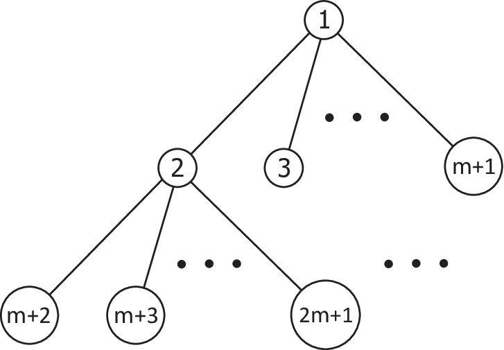
A full $m$ -ary tree is a rooted tree in which every vertex other than the leaves has $m$ children ( $2$ -ary and $3$ -ary trees are sometimes called binary and ternary trees, respectively [GodsilRo_book01]). The depth $\delta$ of a vertex is the length of the path from the root to the vertex. The set of all vertices at a given depth is called a level of the tree: by definition, the root vertex is at depth zero. The number of vertices of a full $m$ -ary tree is $n=\sum_{i=0}^{\delta}m^{i}$ .

Proposition 3 (Full $m$ -ary tree)

For the full $m$ -ary tree, with $m\geq 2$ (see Fig. 2(c)), we have that:

•

For $|s|<1$ , system (2) is asymptotically stable.
•

For $|s|>1$ , system (2) is unstable.

•

For $s=-1$ , system (2) is marginally stable. In this case, the states associated to the vertices in the even levels of the tree asymptotically converge to $\frac{1}{n}\,{\mathbf{x}}_{0}^{T}{\mathbf{h}}$ while the states associated to the vertices in the odd levels of the tree converge to $-\frac{1}{n}\,{\mathbf{x}}_{0}^{T}{\mathbf{h}}$ , where,

{\mathbf{h}}\,\triangleq\,[-1,\,\mathds{1}^{T}_{m},\,-\mathds{1}^{T}_{m^{2}},\,\mathds{1}^{T}_{m^{3}},\,-\mathds{1}^{T}_{m^{4}},\,\mathds{1}^{T}_{m^{5}},\,\ldots\,]^{T}\in\mathop{{\rm I}\mskip-4.0mu{\rm R}}\nolimits^{n}.

Proof: The stability properties of (2) are determined in this case by only one of the eigenvalues of $-\boldsymbol{\Delta}(s)$ (in fact, the other $n-1$ are negative for all $s$ : note that $\det(-\boldsymbol{\Delta}(s))=s^{2}-1$ ). This eigenvalue is negative for $|s|<1$ , positive for $|s|>1$ and zero for $s\in\{-1,\,+1\}$ . For $s=-1$ , note that,

\qquad\quad\;\lim_{t\,\rightarrow\,\infty}\;\exp(-\boldsymbol{\Delta}(-1)\,t)\,{\mathbf{x}}_{0}\,=\,\frac{1}{n}\,{\mathbf{h}}\,{\mathbf{h}}^{T}{\mathbf{x}}_{0}.\qquad\quad\;\hfill\blacksquare

Proposition 4 (Wheel graph $W_{n}$ )

Consider a wheel graph $W_{n}$ with $n>3$ vertices where vertex 1 is the center of the wheel (see Fig. 2(d)), and let $\mu$ be the non-unitary root of

\!-\frac{n}{2}\,s^{2}\,+\,s\,+\,\frac{\sqrt{\big((n-4)\,s+2\big)^{2}+4(n-1)}}{2}\,\,s\,-\,1.

(6)

$\mu$ monotonically decreases from $1/2$ (for $n=4$ ) to $0$ (for $n=\infty$ ) [see Fig. 3]. We have that:

•

For $s>1$ or $s<\mu$ , system (2) is asymptotically stable.
•

For $s\in(\mu,\,1)$ , system (2) is unstable.
•

For $s=\mu$ , system (2) is marginally stable. If $n=4$ average consensus is achieved. Instead, if $n>4$ the state associated to vertex 1 asymptotically converges to ${\mathbf{x}}^{T}_{0}[\alpha^{2},\,\alpha\beta,\,\ldots,\alpha\beta]^{T}$ , and the states associated to the other $n-1$ vertices converge to ${\mathbf{x}}^{T}_{0}[\alpha\beta,\,\beta^{2},\,\ldots,\beta^{2}]^{T}$ , where $[\alpha,\,\beta,\,\ldots,\beta]^{T}$ , $\alpha,\,\beta\in\mathop{{\rm I}\mskip-4.0mu{\rm R}}\nolimits$ , is the unit-norm eigenvector associated to the zero eigenvalue of $-\boldsymbol{\Delta}(\mu)$ .

Proof: The eigenvalues of matrix $-\boldsymbol{\Delta}(s)$ are:

\begin{array}[]{l}\!\!\displaystyle\lambda_{1}(s)=-\frac{n}{2}\,s^{2}\!+s+\!\frac{\sqrt{\big((n-4)\,s+2\big)^{2}+4(n-1)}}{2}\,s-\!1,\\ \!\!\displaystyle\lambda_{2}(s)=-\frac{n}{2}\,s^{2}\!+s-\!\frac{\sqrt{\big((n-4)\,s+2\big)^{2}+4(n-1)}}{2}\,s-\!1,\\ \!\!\lambda_{i+1}(s)=-2s^{2}+2\cos\!\big(\frac{2\pi(i-1)}{n-1}\big)s-1,\,i\in\!\{2,\ldots,n-1\}.\end{array}

Note that the coordinates of the vertex of the parabola $\lambda_{i+1}(s)$ , $i\in\!\{2,\ldots,n-1\}$ , are,

\left[\frac{1}{2}\cos\!\Big(\frac{2\,\pi(i-1)}{n-1}\Big),\;-\frac{1}{2}\Big(1+\sin^{2}\!\Big(\frac{2\,\pi(i-1)}{n-1}\,\Big)\Big)\right],

therefore $\lambda_{i+1}(s)<0$ , $\forall\,s\in\mathop{{\rm I}\mskip-4.0mu{\rm R}}\nolimits$ , $\forall\,i\in\!\{2,\ldots,n-1\}$ . We also have that $\lambda_{2}(s)<0$ , $\forall\,s\in\mathop{{\rm I}\mskip-4.0mu{\rm R}}\nolimits$ . Finally, it is easy to verify that $\lambda_{1}(s)$ has always two roots, $s=\mu$ and $s=1$ . $\lambda_{1}(s)>0$ for $s\in(\mu,\,1)$ and $\lambda_{1}(s)<0$ for $s>1$ or $s<\mu$ . $\blacksquare$

Graph name	Asymptotic stability for :	Marginal stability for :
Path graph $P_{n}$ , $n\geq 2$	$\|s\|<1$	$s=-1$ (2 groups of vertices)
Cycle graph $C_{n}$ , $n>2$ , $n$ even	$\forall\,s\in\,\mathop{{\rm I}\mskip-4.0mu{\rm R}}\nolimits\setminus\{-1,\,1\}$	$s=-1$ (2 groups of vertices)
Cycle graph $C_{n}$ , $n>2$ , $n$ odd	$\forall\,s\in\,\mathop{{\rm I}\mskip-4.0mu{\rm R}}\nolimits\setminus\{1\}$
Full $m$ -ary tree, $m\geq 2$	$\|s\|<1$	$s=-1$ (2 groups of vertices)
Wheel graph $W_{n}$ , $n>3$	$s>1$ or $s<\mu$	$s=\mu$ (2 groups of vertices for $n>4$ )
$m$ -cube, $Q_{m}$ , $n\,=\,2^{m}>4$	$\|s\|>1$ or $\|s\|<\frac{1}{m-1}$	$s\in\{-1,-\frac{1}{m-1}\}$ (2 groups of vertices)
$m$ -cube, $Q_{m}$ , $n\,=\,2^{m}>4$	$\|s\|>1$ or $\|s\|<\frac{1}{m-1}$	$s=\frac{1}{m-1}$ (average consensus)
Petersen graph	$s>1$ or $s<1/2$	$s=1/2$ (average consensus)
Complete graph $K_{n}$ , $n>2$	$s>1$ or $s<\frac{1}{n-2}$	$s=\frac{1}{n-2}$ (average consensus)
$\begin{array}[]{c}\text{Complete bipartite graph}\\ K_{m,n},\,m,n\geq 2\end{array}$	$\|s\|>1$ or $\|s\|<\frac{1}{\sqrt{(m-1)(n-1)}}$	$s\in\{-1,\,-\frac{1}{\sqrt{(m-1)(n-1)}}\}$ (2 groups of vertices)
	$\|s\|>1$ or $\|s\|<\frac{1}{\sqrt{(m-1)(n-1)}}$	$s=\frac{1}{\sqrt{(m-1)(n-1)}}$ $\begin{array}[]{l}(\text{if}\;\,m=n,\;\,\text{average consensus})\\ (\text{if}\;\,m\neq n,\;\,\text{2 groups of vertices})\end{array}$
Star graph $K_{1,n}$ , $n\geq 3$	$\|s\|<1$	$s=-1$ (2 groups of vertices)

Table 1: Summary of the stability properties of the deformed consensus protocol (2), for some special families of undirected graphs. Average consensus is achieved in all cases for

s=1

Proposition 5 ( $m$ -cube $Q_{m}$ )

For the $m$ -cube (or hypercube) graph $Q_{m}$ with $n=2^{m}>4$ vertices (see Fig. 2(e)), we have that⁵⁵ 5 $m$ -cube or hypercube graphs should not be confused with cubic graphs which are 3-regular graphs. The only hypercube which is a cubic graph is $Q_{3}$ .:

•

For $|s|>1$ or $|s|<\frac{1}{m-1}$ , system (2) is asymptotically stable.
•

For $s\in\big(\!-1,\,-\frac{1}{m-1}\big)$ or $s\in\big(\frac{1}{m-1},\,1\big)$ , system (2) is unstable.
•

For $s=\frac{1}{m-1}$ , average consensus is achieved. The convergence rate to $\frac{1}{n}\,{\mathbf{x}}_{0}^{T}\mathds{1}_{n}$ is slower for $s=\frac{1}{m-1}$ than for $s=1$ .
•

For $s\in\{-1,\,-\frac{1}{m-1}\}$ , system (2) is marginally stable. In this case, the states associated to $n/2$ vertices asymptotically converge to $\frac{1}{\sqrt{n}}\,{\mathbf{x}}_{0}^{T}{\mathbf{u}}_{1}$ , while the states associated to the other $n/2$ vertices converge to $-\frac{1}{\sqrt{n}}\,{\mathbf{x}}_{0}^{T}{\mathbf{u}}_{1}$ , where ${\mathbf{u}}_{1}$ is the unit-norm eigenvector associated to the zero eigenvalue of $-\boldsymbol{\Delta}(-1)$ or $-\boldsymbol{\Delta}(-\frac{1}{m-1})$ .

Proof: Since the eigenvalues of the adjacency matrix of the $m$ -cube are the numbers $m-2\ell$ with multiplicity $\left(\begin{smallmatrix}m\vskip 2.84544pt\\ \ell\end{smallmatrix}\right)$ , $\ell\in\{0,\ldots,m\}$ [BrouwerHa_book12, Sect. 1.4.6], then from Lemma 1, the eigenvalues of matrix $-\boldsymbol{\Delta}(s)$ are $-(m-1)\,s^{2}+(m-2\ell)\,s-1$ with multiplicity $\left(\begin{smallmatrix}m\vskip 2.84544pt\\ \ell\end{smallmatrix}\right)$ . The stability of system (2) is only determined by the eigenvalues,

\begin{array}[]{l}\lambda_{1}(s)\,=\,-(m-1)\,s^{2}\,+\,m\,s\,-\,1,\\ \lambda_{n}(s)\,=\,-(m-1)\,s^{2}\,-\,m\,s\,-\,1,\end{array}

since the other $n-2$ eigenvalues are negative for all $s$ . We have that $\lambda_{1}(s)<0$ for $s>1$ or $s<\frac{1}{m-1}$ . Instead, $\lambda_{n}(s)<0$ for $s>-\frac{1}{m-1}$ or $s<-1$ . Hence, for $|s|>1$ or $|s|<\frac{1}{m-1}$ , system (2) is asymptotically stable and for $s\in\{-1,\,\pm\frac{1}{m-1}\}$ , marginal stability is achieved. Note in particular, that $\boldsymbol{\Delta}\big(\!-\!\frac{1}{m-1}\big)=\frac{1}{m-1}\,\boldsymbol{\Delta}(-1)$ and that for a suitable labeling of the vertices of the graph, we have

\!\lim\limits_{t\,\rightarrow\,\infty}\,\,\exp(-\boldsymbol{\Delta}(-1)\,t)\,{\mathbf{x}}_{0}\,=\,\frac{1}{n}\left[-\mathds{k},\,\mathds{k},\ldots,\,-\mathds{k},\,\mathds{k}\right]{\mathbf{x}}_{0}.

Finally, note that $\boldsymbol{\Delta}\big(\frac{1}{m-1}\big)=\frac{1}{m-1}\,\boldsymbol{\Delta}(1)=\frac{1}{m-1}\,{\mathbf{L}}$ which implies that $\lambda_{2}\big(\boldsymbol{\Delta}\big(\frac{1}{m-1}\big)\big)\,=\,\frac{1}{m-1}\,\,\lambda_{2}\left(\boldsymbol{\Delta}(1)\right)$ . If we now recall the role played by the algebraic connectivity of the graph in the consensus protocol, we have that the convergence rate to $\frac{1}{n}\,{\mathbf{x}}_{0}^{T}\mathds{1}_{n}$ is slower for $s=\frac{1}{m-1}$ than for $s=1$ . $\blacksquare$

Proposition 6 (Petersen graph)

For the Petersen graph (see Fig. 2(f)), we have that:

•

For $s>1$ or $s<1/2$ , system (2) is asymptotically stable.
•

For $s\in(1/2,\,1)$ , system (2) is unstable.
•

For $s=1/2$ , average consensus is achieved. The convergence rate to $\frac{1}{10}\,{\mathbf{x}}_{0}^{T}\mathds{1}_{10}$ is slower for $s=1/2$ than for $s=1$ .

Proof: Since the eigenvalues of the adjacency matrix of the Petersen graph are $3$ , $1$ and $-2$ with multiplicity 1, 5 and 4, respectively [BrouwerHa_book12, Sect. 1.4.5], then from Lemma 1, the eigenvalues of $-\boldsymbol{\Delta}(s)$ are:

\begin{array}[]{lll}\displaystyle\lambda_{1}(s)&=&-2\,s^{2}+3\,s-1,\\ \displaystyle\lambda_{2}(s)&=&\ldots\,=\,\lambda_{6}(s)=-2\,s^{2}+s-1,\\ \displaystyle\lambda_{7}(s)&=&\ldots\,=\,\lambda_{10}(s)=-2\,s^{2}-2\,s-1.\end{array}

We have that $\lambda_{2}(s)<0$ and $\lambda_{7}(s)<0$ , $\forall\,s\in\mathop{{\rm I}\mskip-4.0mu{\rm R}}\nolimits$ . Moreover, $\lambda_{1}(s)<0$ for $s>1$ or $s<1/2$ , and the unit-norm eigenvector associated to $\lambda_{1}(1/2)$ is $\frac{1}{\sqrt{10}}\,\mathds{1}_{10}$ . Finally, $\boldsymbol{\Delta}(1/2)=\frac{1}{2}\,\boldsymbol{\Delta}(1)$ , hence the convergence rate to $\frac{1}{10}\,{\mathbf{x}}_{0}^{T}\mathds{1}_{10}$ is slower for $s=1/2$ than for $s=~1$ . $\blacksquare$

Proposition 7 (Complete graph $K_{n}$ )

For the complete graph $K_{n}$ with $n>2$ vertices (see Fig. 2(g)), we have that:

•

For $s>1$ or $s<\frac{1}{n-2}$ , system (2) is asymptotically stable.
•

For $s\in\big(\frac{1}{n-2},\,1\big)$ , system (2) is unstable.
•

For $s=\frac{1}{n-2}$ , average consensus is achieved. The convergence rate to $\frac{1}{n}\,{\mathbf{x}}_{0}^{T}\mathds{1}$ is slower for $s=\frac{1}{n-2}$ than for $s=1$ .

Proof: Since the eigenvalues of the adjacency matrix of the complete graph are $n-1$ and $-1$ with multiplicity $1$ and $n-1$ , respectively [BrouwerHa_book12, Sect. 1.4.1], then from Lemma 1 the eigenvalues of $-\boldsymbol{\Delta}(s)$ are:

\begin{array}[]{lll}\displaystyle\lambda_{1}(s)&=&-(n-2)\,s^{2}+(n-1)\,s-1,\\ \displaystyle\lambda_{2}(s)&=&\ldots\,=\;\lambda_{n}(s)\,=\,-(n-2)\,s^{2}-s-1.\end{array}

We have that $\lambda_{2}(s)<0$ , $\forall\,s\in\mathop{{\rm I}\mskip-4.0mu{\rm R}}\nolimits$ . Moreover, $\lambda_{1}(s)<0$ for $s>1$ or $s<\frac{1}{n-2}$ , and the unit-norm eigenvector associated to $\lambda_{1}\big(\frac{1}{n-2}\big)$ is $\frac{1}{\sqrt{n}}\,\mathds{1}$ . Finally, note that $\boldsymbol{\Delta}\big(\frac{1}{n-2}\big)=\frac{1}{n-2}\,\boldsymbol{\Delta}(1)$ , hence, the convergence rate to $\frac{1}{n}\,{\mathbf{x}}_{0}^{T}\mathds{1}$ is slower for $s=\frac{1}{n-2}$ than for $s=1$ . $\blacksquare$

Proposition 8 (Complete bipartite graph $K_{m,n}$ )

For the complete bipartite graph $K_{m,n}=(V_{1}\cup V_{2},E)$ , where $|V_{1}|=m$ , $|V_{2}|=n$ with $m,n\geq 2$ (see Fig. 2(h)), we have that:

•

For $|s|>1$ or $|s|<\frac{1}{\sqrt{(m-1)(n-1)}}$ , system (2) is asymptotically stable.
•

For $s\in\big(-1,-\frac{1}{\sqrt{(m-1)(n-1)}}\big)$ or $s\in\big(\frac{1}{\sqrt{(m-1)(n-1)}},1\big)$ , system (2) is unstable.
•
For $s\in\big\{\!-1,\,\,\pm\frac{1}{\sqrt{(m-1)(n-1)}}\big\}$ , system (2) is marginally stable. In particular, given the initial condition ${\mathbf{x}}_{0}\in\mathop{{\rm I}\mskip-4.0mu{\rm R}}\nolimits^{m+n}$ :
- –
  
  If $m\neq n$ : for $s=-1$ , the states associated to the vertices in $V_{1}$ asymptotically converge to $\frac{1}{m+n}\,{\mathbf{x}}_{0}^{T}[\mathds{1}^{T}_{m},-\!\mathds{1}^{T}_{n}]^{T}$ and the states associated to the vertices in $V_{2}$ converge to $-\frac{1}{m+n}\,{\mathbf{x}}_{0}^{T}[\mathds{1}^{T}_{m},-\!\mathds{1}^{T}_{n}]^{T}$ .
  For $s=\pm\frac{1}{\sqrt{(m-1)(n-1)}}$ , the states associated to the vertices in $V_{1}$ and $V_{2}$ asymptotically converge to one of the two different values taken by the components of the vector $({\mathbf{u}}_{1}\,{\mathbf{u}}^{T}_{1})\,{\mathbf{x}}_{0}$ , where ${\mathbf{u}}_{1}$ is the unit-norm eigenvector associated to the zero eigenvalue of $-\boldsymbol{\Delta}\big(\pm\frac{1}{\sqrt{(m-1)(n-1)}}\big)$ .
- –
  
  If $m=n$ : for $s=\frac{1}{n-1}$ average consensus is achieved, and the convergence rate to $\frac{1}{2n}\,{\mathbf{x}}_{0}^{T}\mathds{1}_{2n}$ is slower for $s=\frac{1}{n-1}$ than for $s=1$ . For $s\in\big\{\!\!-1,-\frac{1}{n-1}\big\}$ the states associated to the vertices in $V_{1}$ asymptotically converge to $\frac{1}{2n}\,{\mathbf{x}}_{0}^{T}[\mathds{1}^{T}_{n}\!,-\mathds{1}^{T}_{n}]^{T}$ and the states associated to the vertices in $V_{2}$ converge to $-\frac{1}{2n}\,{\mathbf{x}}_{0}^{T}[\mathds{1}^{T}_{n}\!,-\mathds{1}^{T}_{n}]^{T}$ .

Proof: In this case, the eigenvalues of $-\boldsymbol{\Delta}(s)$ are:

\begin{array}[]{l}\displaystyle\lambda_{1}(s)=-\frac{n+m-2}{2}\,s^{2}+\frac{\sqrt{(n-m)^{2}s^{2}+\,4mn}}{2}\,s\,-\,1,\\ \displaystyle\lambda_{2}(s)=-\frac{n+m-2}{2}\,s^{2}-\frac{\sqrt{(n-m)^{2}s^{2}+\,4mn}}{2}\,s\,-\,1,\end{array}

\begin{array}[]{l}\displaystyle\hskip-34.14322pt\lambda_{3}(s)=\ldots=\lambda_{n+1}(s)=-((m-1)\,s^{2}+1),\\ \displaystyle\hskip-34.14322pt\lambda_{n+2}(s)=\ldots=\lambda_{n+m}(s)=-((n-1)\,s^{2}+1).\end{array}

Since $\lambda_{3}(s)$ , $\ldots$ , $\lambda_{n+m}(s)$ are negative for all $s$ , the stability of system (2) is only determined by the eigenvalues $\lambda_{1}(s)$ and $\lambda_{2}(s)$ . A systematic study of the roots of $\lambda_{1}(s)$ and $\lambda_{2}(s)$ immediately leads to the first two items of the statement. For the marginal-stability case, note that for $s=-1$ :

\!\lim_{t\,\rightarrow\,\infty}\exp\big(-\boldsymbol{\Delta}(-1)\,t\big)\,{\mathbf{x}}_{0}=\frac{1}{m+n}\left[\begin{matrix}\mathds{J}_{m\times m}&-\mathds{J}_{m\times n}\\ -\mathds{J}_{n\times m}&\mathds{J}_{n\times n}\end{matrix}\right]\!{\mathbf{x}}_{0}.

Moreover, observe that if $m=n$ , $\boldsymbol{\Delta}\big(\!-\!\frac{1}{n-1}\big)=\frac{1}{n-1}\,\boldsymbol{\Delta}(-1)$ , and analogously, $\boldsymbol{\Delta}\big(\frac{1}{n-1}\big)=\frac{1}{n-1}\,\boldsymbol{\Delta}(1)$ , hence the rate of convergence to $\frac{1}{2n}\,{\mathbf{x}}_{0}^{T}\mathds{1}_{2n}$ is slower for $s=\frac{1}{n-1}$ than for $s=1$ . $\blacksquare$

From Prop. 8, we can deduce the following result (recall that the star graph is a complete bipartite graph with $m=1$ ):

Proposition 9 (Star graph $K_{1,n}$ )

For the star graph $K_{1,n}$ with $n\geq 3$ , where vertex 1 is the center of the star (see Fig. 2(i)), we have that:

•

For $|s|<1$ , system (2) is asymptotically stable.
•

For $|s|>1$ , system (2) is unstable.
•

For $s=-1$ , system (2) is marginally stable. In this case, the state associated to vertex 1 asymptotically converges to $\frac{1}{n+1}\,{\mathbf{x}}_{0}^{T}[1,-\mathds{1}^{T}_{n}]^{T}$ and the states associated to the other $n$ vertices converge to $-\frac{1}{n+1}\,{\mathbf{x}}_{0}^{T}[1,-\mathds{1}^{T}_{n}]^{T}$ . $\blacksquare$

For the reader’s convenience, all the results found in this section are summarized in Table 1.

Remark 2

Note that the path, cycle (with $n$ even), full $m$ -ary tree, $m$ -cube, complete bipartite and star graphs are all bipartite graphs. Then, in view of Property 2.6, for $s=-1$ the state of system (2) asymptotically converges to $({\mathbf{u}}_{n}{\mathbf{u}}_{n}^{T})\,{\mathbf{x}}_{0}$ with these graphs, where ${\mathbf{u}}_{n}$ is the unit-norm eigenvector associated to the zero eigenvalue of the signless Laplacian ${\mathbf{Q}}$ . According to [Altafini_TAC13, Def. 1], we can say that system (2) admits a bipartite consensus solution in these cases. $\diamond$

3.3 Stability conditions for graphs of arbitrary topology

In order to extend the analysis of the previous section to arbitrary undirected graphs, we briefly review here the spectral theory of quadratic eigenvalues problems (QEPs) [TisseurMe_SIAM01, Sect. 3], that constitute an important class of nonlinear eigenvalue problems. Let

{\mathbf{P}}(\lambda)\,=\,{\mathbf{B}}_{2}\,\lambda^{2}+{\mathbf{B}}_{1}\,\lambda+{\mathbf{B}}_{0},

be an $n\times n$ matrix polynomial of degree 2, where ${\mathbf{B}}_{2}$ , ${\mathbf{B}}_{1}$ and ${\mathbf{B}}_{0}$ are $n\times n$ complex matrices [GohbergLaRo_Book09]. In other words, the components of the matrix ${\mathbf{P}}(\lambda)$ are quadratic polynomials in the variable $\lambda$ .

Definition 11 (Spectrum of ${\mathbf{P}}(\lambda)$ )

The spectrum of ${\mathbf{P}}(\lambda)$ , denoted by $\Sigma({\mathbf{P}})$ , is defined as,

\Sigma({\mathbf{P}})=\{\,\lambda\in\mathbb{C}\,:\,\det({\mathbf{P}}(\lambda))=0\},

i.e., it is the set of eigenvalues of ${\mathbf{P}}(\lambda)$ [TisseurMe_SIAM01]. $\diamond$

Definition 12 (Regular ${\mathbf{P}}(\lambda)$ )

The matrix ${\mathbf{P}}(\lambda)$ is called regular when $\det({\mathbf{P}}(\lambda))$ is not identically zero for all values of $\lambda$ , and nonregular otherwise [TisseurMe_SIAM01]. $\diamond$

Note that $\det({\mathbf{P}}(\lambda))=\det({\mathbf{B}}_{2})\lambda^{2n}+$ lower-order terms, so when ${\mathbf{B}}_{2}$ is nonsingular, ${\mathbf{P}}(\lambda)$ is regular and has $2n$ finite eigenvalues. When ${\mathbf{B}}_{2}$ is singular, the degree of $\det({\mathbf{P}}(\lambda))$ is $r<2n$ and ${\mathbf{P}}(\lambda)$ has $r$ finite eigenvalues and $2n-r$ infinite eigenvalues⁶⁶ 6 The infinite eigenvalues correspond to the zero eigenvalues of the reverse polynomial $\lambda^{2}\,{\mathbf{P}}(\lambda^{-1})={\mathbf{B}}_{0}\,\lambda^{2}+{\mathbf{B}}_{1}\,\lambda+{\mathbf{B}}_{2}$ .. The algebraic multiplicity of an eigenvalue $\lambda_{0}$ is the order of the corresponding zero in $\det({\mathbf{P}}(\lambda))$ , while the geometric multiplicity of $\lambda_{0}$ is the dimension of $\ker({\mathbf{P}}(\lambda_{0}))$ .

Problem 1 (Quadratic eigenvalue problem, QEP)

The QEP consists of finding scalars $\lambda$ and nonzero vectors ${\mathbf{z}}$ , ${\mathbf{y}}$ , satisfying [TisseurMe_SIAM01],

{\mathbf{P}}(\lambda)\,{\mathbf{z}}={\mathbf{0}},\quad\,{\mathbf{y}}^{*}\,{\mathbf{P}}(\lambda)={\mathbf{0}},

where ${\mathbf{z}}$ , ${\mathbf{y}}\in\mathbb{C}^{n}$ are respectively the right and left eigenvector corresponding to the eigenvalue $\lambda\in\mathbb{C}$ , and ${\mathbf{y}}^{*}$ is the conjugate transpose of ${\mathbf{y}}$ . $\diamond$

A QEP has $2n$ eigenvalues (finite or infinite) with up to $2n$ right and $2n$ left eigenvectors. Note that a regular ${\mathbf{P}}(\lambda)$ may possess two distinct eigenvalues having the same eigenvector. If a regular ${\mathbf{P}}(\lambda)$ has $2n$ distinct eigenvalues, then there exists a set of $n$ linearly independent eigenvectors.

Property 3 (Spectral properties of ${\mathbf{P}}(\lambda)$ )

If matrices ${\mathbf{B}}_{2}$ , ${\mathbf{B}}_{1}$ , ${\mathbf{B}}_{0}$ are real symmetric, the eigenvalues of ${\mathbf{P}}(\lambda)$ are either real or occur in complex-conjugate pairs, and the sets of left and right eigenvectors coincide [TisseurMe_SIAM01]. $\diamond$

By leveraging the previous facts (note that according to Def. 12, $\boldsymbol{\Delta}(\lambda)$ is a regular matrix since we always have $\det(\boldsymbol{\Delta}(\lambda))\neq 0$ for $\lambda=0$ ), we deduce the following property of the deformed consensus protocol (2):

Proposition 10

The finite real eigenvalues $\lambda$ of the QEP,

(({\mathbf{I}}_{n}-{\mathbf{D}})\,\lambda^{2}+{\mathbf{A}}\,\lambda-{\mathbf{I}}_{n})\,{\mathbf{z}}\,=\,{\mathbf{0}},

(7)

are the values of $s$ for which system (2) is marginally stable. Moreover, if $\lambda$ is one of these eigenvalues with geometric multiplicity one, and $\overline{{\mathbf{z}}}={\mathbf{z}}/\|{\mathbf{z}}\|$ is the associated unit-norm eigenvector, we have that:

\hskip 68.28644pt\lim_{t\rightarrow\infty}\,{\mathbf{x}}(t)\;=\;(\overline{{\mathbf{z}}}\,\,\overline{{\mathbf{z}}}^{T})\,{\mathbf{x}}_{0}.\hskip 62.59596pt\hfill\blacksquare

Remark 3 (Computation of the eigenvalues)

The eigenvalues of the QEP (7) can be easily computed by converting it to a standard generalized eigenvalue problem⁷⁷ 7 This construction is called “linearization” in the literature and it is not unique in general (see [Demmel_book97, Sect. 4.5]). of size $2n$ , by defining the new vector ${\mathbf{w}}=\lambda\,{\mathbf{z}}$ . In terms of ${\mathbf{z}}$ and ${\mathbf{w}}$ , problem (7) becomes:

\qquad\;\left[\,\begin{matrix}{\mathbf{0}}\;&\;{\mathbf{I}}_{n}\\ {\mathbf{I}}_{n}\;&\;-{\mathbf{A}}\\ \end{matrix}\,\right]\!\left[\,\begin{matrix}{\mathbf{z}}\\ {\mathbf{w}}\end{matrix}\,\right]\,=\,\lambda\!\left[\,\begin{matrix}{\mathbf{I}}_{n}\;&\;{\mathbf{0}}\\ {\mathbf{0}}\;&\;{\mathbf{I}}_{n}-{\mathbf{D}}\\ \end{matrix}\,\right]\!\left[\,\begin{matrix}{\mathbf{z}}\\ {\mathbf{w}}\end{matrix}\,\right]\!.

Matlab’s function “polyeig” uses a linearization procedure similar to the one described above, to numerically solve generic polynomial eigenvalue problems. Note that if matrix ${\mathbf{I}}_{n}-{\mathbf{D}}$ is singular, it is more convenient, from a numerical viewpoint, to use the second instead of the first companion form considered above, for the linearization (cf. [TisseurMe_SIAM01, Sect. 3.4]). $\diamond$

The following proposition elucidates the connection existing between the topology of the communication graph $\mathcal{G}$ , and the properties of the QEP (7).

Proposition 11

If the graph $\mathcal{G}$ has a vertex with degree equal to one (i.e. only one edge is incident to that vertex), ${\mathbf{I}}_{n}-{\mathbf{D}}$ is singular and the QEP (7) admits at least two infinite eigenvalues. $\blacksquare$

For example, with the path graph $\text{rank}({\mathbf{I}}_{n}-{\mathbf{D}})=n-2$ , with the star graph $\text{rank}({\mathbf{I}}_{n}-{\mathbf{D}})=1$ and with the full $m$ -ary tree graph $\text{rank}({\mathbf{I}}_{n}-{\mathbf{D}})=n-m^{\delta}$ : in the first two cases $\det(({\mathbf{I}}_{n}-{\mathbf{D}})\lambda^{2}+{\mathbf{A}}\,\lambda-{\mathbf{I}}_{n})=(-1)^{n-1}(\lambda^{2}-1)$ , while in the last $\det(({\mathbf{I}}_{n}-{\mathbf{D}})\lambda^{2}+{\mathbf{A}}\,\lambda-{\mathbf{I}}_{n})=\lambda^{2}-1$ . Hence, in all cases, the QEP (7) admits $2n-2$ infinite eigenvalues.
The next proposition, the last result of this section, shows how to determine the $s$ -stability interval of the deformed consensus protocol, for graphs with arbitrary topology (see Fig. 4).

Proposition 12 (Stability interval for arbitrary $\mathcal{G}$ )

Let $q(s)\,\triangleq\,\det(({\mathbf{I}}_{n}-{\mathbf{D}})\,s^{2}+{\mathbf{A}}\,s-{\mathbf{I}}_{n})$ , then:

•

If $n$ is even, system (2) is asymptotically stable for all $s$ such that $q(s)>0$ , and unstable for all $s$ such that $q(s)<0$ .
•

If $n$ is odd, system (2) is asymptotically stable for all $s$ such that $q(s)<0$ , and unstable for all $s$ such that $q(s)>0$ .

Proof: From Property 3 and Property 1.1, it follows that:

q(s)\,=\,(s-1)\prod_{k=1}^{\ell}(s-\zeta_{k})(s-\zeta_{k}^{*})\prod_{j\,=\,1}^{r-\,2\ell-1}(s-\eta_{j}),

where $r\leq 2n$ is the degree of $q(s)$ , $(\zeta_{k},\,\zeta_{k}^{*})$ are the $\ell$ pairs of complex-conjugate roots of $q(s)$ and $\eta_{j}$ the $r-2\ell-1$ non-unitary real roots of $q(s)$ (counted with their multiplicity). Since $\prod_{k=1}^{\ell}(s-\zeta_{k})(s-\zeta_{k}^{*})=\prod_{k=1}^{\ell}s^{2}-2\Re[\zeta_{k}]\,s+|\zeta_{k}|^{2}>0$ for all $s$ , where $\Re[\,\cdot\,]$ denotes the real part of a complex number, the statement follows from Prop. 10. $\blacksquare$

The following example illustrates the rich variety of behaviors exhibited by the deformed consensus protocol on four “generic” (nonbipartite) graphs with five vertices.

Example 1

Consider the four graphs reported in Fig. 5. By leveraging Prop. 10 and Prop. 12, we have that:

•

With the graph in Fig. 5(a), system (2) is asymptotically stable $\forall\,s\in\mathop{{\rm I}\mskip-4.0mu{\rm R}}\nolimits\setminus\{1\}$ .
•

With the graph in Fig. 5(b), system (2) is asymptotically stable for $s<0.7022$ or $s>1$ . For $s=0.7022$ , the system is marginally stable and three groups of vertices can be identified: $\{1\}$ , $\{2,5\}$ , $\{3,4\}$ (different shapes are used in Fig. 5(b) to indicate these groups).
•

With the graph in Fig. 5(c), system (2) is asymptotically stable for $s<0.4396$ or $s>1$ . For $s=0.4396$ , the system is marginally stable and three groups of vertices can be identified: $\{1\}$ , $\{2,5\}$ , $\{3,4\}$ .
•

With the graph in Fig. 5(d), system (2) is asymptotically stable for $s<0.3804$ or $s>1$ . For $s=0.3804$ , the system is marginally stable and two groups of vertices can be identified: $\{1,3\}$ , $\{2,4,5\}$ .

From Figs. 5(b)-(d), we notice that vertices in the same group tend to have the same edge degree, and that an increase in the algebraic connectivity of the graph leads to a shrinkage of the $s$ -stability interval of the deformed consensus protocol. In future works, we will delve into the peculiar grouping behavior exhibited by the vertices of the four graphs considered in this example. $\diamond$

4 Extensions

In this section, two extensions to the theory presented in Sect. 3 are discussed: we first briefly consider a discrete-time version of the deformed consensus protocol (2), and then deal with directed communication graphs.

4.1 Discrete-time deformed consensus protocol

Following [OlfatiFaMu_IEEE07, Sect. IIC], we can introduce the following discrete-time version of protocol (2),

{\mathbf{x}}(k+1)\,=\,\mathds{P}(s)\,{\mathbf{x}}(k),\;\;k\in\{0,\,1,\,2,\ldots\},

(8)

where

\mathds{P}(s)\,=\,{\mathbf{I}}_{n}-\epsilon\,\boldsymbol{\Delta}(s),

is the deformed Perron matrix and $0<\epsilon<1/d_{\max}$ is the step-size, where $d_{\max}=\max_{\,i}\,(\sum_{j\neq i}a_{ij})$ is the maximum degree of $\mathcal{G}$ . It is easy to verify that the continuous-time and discrete-time deformed consensus protocols share the same $s$ -stability intervals, and thus the analysis of Sect. 3, mutatis mutandis, is still valid for system (8).

4.2 Deformed consensus protocol for directed graphs

In this section we assume that the communication graph is directed and contains a rooted out-branching, and by mimicking Sect. 3 we will study the stability properties of the following linear system,

\dot{{\mathbf{x}}}(t)=-\boldsymbol{\Delta}(\mathcal{D}(s))\,{\mathbf{x}}(t),

(9)

in terms of the real parameter $s$ , where the symbol “ $\mathcal{D}(s)$ ” indicates that the deformed Laplacian is now relative to a directed communication topology. Similarly to Sect. 3.1, we have here that:

\boldsymbol{\Delta}(\mathcal{D}(1))\,=\,{\mathbf{L}}(\mathcal{D}),\quad\;\boldsymbol{\Delta}(\mathcal{D}(-1))\,=\,{\mathbf{Q}}(\mathcal{D}).

It is well known [MesbahiEg_book10], that if the digraph $\mathcal{D}$ contains a rooted out-branching, the state trajectory of system,

\dot{{\mathbf{x}}}(t)=-{\mathbf{L}}(\mathcal{D})\,{\mathbf{x}}(t),

(10)

satisfies,

\lim_{t\rightarrow\infty}\;{\mathbf{x}}(t)\,=\,(\overline{{\mathbf{u}}}_{1}\overline{{\mathbf{v}}}^{T}_{1})\,{\mathbf{x}}_{0},

where $\overline{{\mathbf{u}}}_{1}$ and $\overline{{\mathbf{v}}}_{1}$ , are, respectively, the right and left eigenvectors associated with the zero eigenvalue of ${\mathbf{L}}(\mathcal{D})$ , normalized such that $\overline{{\mathbf{u}}}^{T}_{1}\overline{{\mathbf{v}}}_{1}=1$ . Moreover, we have that (10) reaches average consensus for every initial state if and only if $\mathcal{D}$ is weakly connected and balanced.
In what follows, we will analyze the stability properties of system (9) for two special families of directed graphs, and briefly explore the case of digraphs of arbitrary topology with the help of few significative examples.

Proposition 13 (Directed path)

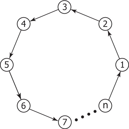
For the directed path graph with $n\geq 2$ vertices (see Fig. 6(a)), we have that:

•

For $|s|<1$ , system (9) is asymptotically stable.
•

For $|s|>1$ , system (9) is unstable.
•
For $s\in\{-1,\,+1\}$ , system (9) is marginally stable.
- –
  
  For $s=-1$ , it is possible to identify two groups of $n/2$ vertices (if $n$ is even), or one group of $\lfloor n/2\rfloor$ vertices and one of $\lfloor n/2\rfloor+1$ vertices (if $n$ is odd). The states associated to the vertices in one group reach an agreement on $x_{1}(0)$ , and the states associated to the vertices in the other group agree on $-x_{1}(0)$ .
- –
  
  For $s=1$ , the consensus value is $x_{1}(0)$ .

Proof: In this case, $-\boldsymbol{\Delta}(\mathcal{D}(s))$ is a lower-triangular matrix,

-\boldsymbol{\Delta}(\mathcal{D}(s))\,=\left[\,\begin{matrix}s^{2}\!-\!1&&&&&\vskip-4.26773pt\\ s&\,-1&&&&\vskip-2.84544pt\\ &&&\ddots&&\vskip-4.26773pt\\ &&&s\;\;&\;\,-1&\vskip-4.26773pt\\ &&&&s\;\;&\;\,-1\end{matrix}\,\right],

whose eigenvalues are,

\lambda_{1}(s)=s^{2}-1,\quad\lambda_{2}(s)=\,\ldots\,=\lambda_{n}(s)=-1,

from which the first two items of the statement immediately follow. For the marginal-stability case, note that,

\lim_{t\,\rightarrow\,\infty}\;\exp(-\boldsymbol{\Delta}(\mathcal{D}(-1))\,t)\,{\mathbf{x}}_{0}\,=\,\big[\!-\mathds{k},\,\,{\mathbf{0}}_{n\times(n-1)}\big]\,{\mathbf{x}}_{0},

and

\lim_{t\,\rightarrow\,\infty}\exp(-\boldsymbol{\Delta}(\mathcal{D}(1))\,t)\,{\mathbf{x}}_{0}=\big[\mathds{1},\,{\mathbf{0}}_{n\times(n-1)}\big]\,{\mathbf{x}}_{0}=x_{1}(0)\,\mathds{1}.\vskip-8.5359pt

$\blacksquare$

Protocol (9) exhibits a richer set of behaviors with directed cycle graphs, as detailed in the next proposition.

Digraph name	Asymptotic stability for :	Marginal stability for :
Directed path, $n\geq 2$	$\|s\|<1$	$\begin{array}[]{c}s=-1\;\,\text{(2 groups of vertices)}\\ s=1\;\,\text{(consensus)}\end{array}$
Directed cycle $\emph{\textsf{D}}_{n}$ , $n>2$ , $n$ even	$\|s\|<1$	$\begin{array}[]{c}s=-1\;\,\text{(2 groups of vertices)}\\ s=1\;\,\text{(average consensus)}\end{array}$
Directed cycle $\emph{\textsf{D}}_{n}$ , $n>2$ , $n$ odd	$s\in(\vartheta(n),\,1)$	$\begin{array}[]{c}s=\vartheta(n)\;\,\text{(stable oscillations)}\\ s=1\;\,\text{(average consensus)}\end{array}$

Table 2: Summary of the stability properties of the deformed consensus protocol (9), for two families of directed graphs.

Proposition 14 (Directed cycle $\textsf{D}_{n}$ )

For the directed cycle graph $\textsf{D}_{n}$ with $n>2$ vertices (see Fig. 6(b)), we have that:

•

For $s=1$ and for all $n>2$ , average consensus is achieved.
•
If $n$ is even:
- –
  
  For $|s|<1$ , system (9) is asymptotically stable.
- –
  
  For $|s|>1$ , system (9) is unstable.
- –
  
  For $s=-1$ , system (9) is marginally stable. In this case, the states associated to $n/2$ vertices asymptotically converge to $\frac{1}{n}\,{\mathbf{x}}_{0}^{T}\,\mathds{k}$ and the states associated to the other $n/2$ vertices converge to $-\frac{1}{n}\,{\mathbf{x}}_{0}^{T}\,\mathds{k}$ .
•
If $n$ is odd:
- –
  
  System (9) is asymptotically stable for $s\in(\vartheta(n),\,1)$ , where,
  
  $\vartheta(n)\,=\,\frac{1}{\displaystyle\cos\!\left(\frac{n(n-2)+1}{n}\,\pi\right)}\,.$
- –
  
  For $s<\vartheta(n)$ or $s>1$ , system (9) is unstable.
- –
  
  For $s=\vartheta(n)$ , system (9) is marginally stable. At steady-state, we have that the $i$ -th state of system (9), $i\in\{1,\ldots,n\}$ , obeys,
  
  $x_{i}(t)\,=\,\textup{A}\sin\!\big(2\pi\,f(n)\,t\,+\,\phi_{i}(n)\,+\,\phi_{\circ}\big),$
  
  where A and $\phi_{\circ}$ are positive constants, the frequency
  
  $f(n)\,=\,\frac{1}{2\pi}\,\tan\!\left(\frac{n(n-2)+1}{n}\,\,\pi\!\right)\!,$
  
  and for $i\in\{1,\ldots,n\}$ , the phase
  
  $\phi_{i}(n)\,=\,\frac{2\pi\,(i-1)}{n\tan\!\Big(\frac{n(n-2)+1}{n}\,\pi\Big)}\,.$

Proof: Similarly to Prop. 2, $-\boldsymbol{\Delta}(\mathcal{D}(s))$ is a circulant matrix in this case,

-\boldsymbol{\Delta}(\mathcal{D}(s))\,=\,\text{circ}[-1,\,0,\,\ldots,\,0,\,s],

and using formula (4) the eigenvalues of $-\boldsymbol{\Delta}(\mathcal{D}(s))$ can be computed in closed-form as,

\lambda_{i}(s)\,=\,s\,\exp\!\left(\frac{2\pi(i-1)(n-1)j}{n}\right)\,-1,\;\;i\in\{1,\ldots,\,n\},

(11)

where $j$ is the imaginary unit. The statement easily follows from a systematic study of (11) in terms of parameter $s$ . In particular, for $s=1$ , $\boldsymbol{\Delta}(\mathcal{D}(s))$ reduces to the standard Laplacian matrix and being $\textsf{D}_{n}$ strongly connected and balanced, average consensus is achieved. If $n$ is even and $s=-1$ ,

\lim_{t\,\rightarrow\,\infty}\exp(-\boldsymbol{\Delta}(\mathcal{D}(-1))\,t)\,{\mathbf{x}}_{0}=\frac{1}{n}\left[-\mathds{k},\,\mathds{k},\,\ldots,\,-\mathds{k},\,\mathds{k}\right]{\mathbf{x}}_{0}.

On the other hand, if $n$ is odd and $s=\vartheta(n)$ , the following pair of purely imaginary eigenvalues appears in (11),

\lambda_{\lceil n/2\rceil,\,\lceil n/2\rceil+1}\,=\,\pm\,j\,\tan\!\left(\frac{n(n-2)+1}{n}\,\pi\right),

where $\lceil\cdot\rceil$ denotes the ceiling function, all the other eigenvalues having negative real parts. $\lambda_{\lceil n/2\rceil}$ , $\lambda_{\lceil n/2\rceil+1}$ are responsible for the periodic solutions of period,

\frac{1}{f(n)}\,=\,\frac{2\pi}{\tan\!\Big(\frac{n(n-2)+1}{n}\,\pi\Big)},

and phase $\phi_{i}(n)$ of system (9), (cf. [Strogatz_book94, p. 134]). $\blacksquare$

Note that $\det(-\boldsymbol{\Delta}(\textsf{D}_{n}(s)))=(-1)^{n}\,(1-s^{n})$ and that the directed path and the directed cycle (for $n$ even), are bipartite digraphs (cf. Prop. 2 and Remark 2).

For easiness of reference, the results found in this section are summarized in Table 2.

Remark 4

Note that differently from Sect. 3, since $\boldsymbol{\Delta}(\mathcal{D}(s))$ is nonsymmetric, it can also admit complex-conjugate eigenvalues and the states of system (9) may experience stable steady-state oscillations (as we have seen in Prop. 14 for $n$ odd). It is worth pointing out here that this is not true, instead, for the protocol (10), which does not admit stable periodic solutions (cf. Prop. 3.10 in [MesbahiEg_book10]). $\diamond$

Since the study of the behavior of system (9) for digraphs $\mathcal{D}$ of arbitrary topology is nontrivial, we will focus here on few representative examples and try to deduce some criteria of general validity.

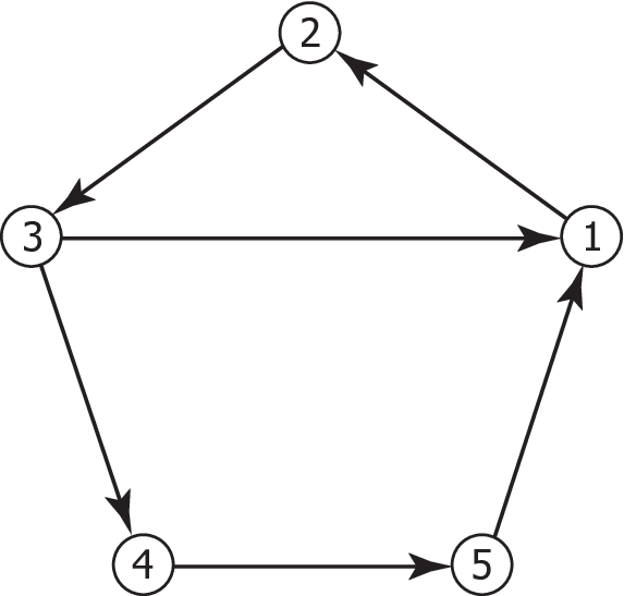
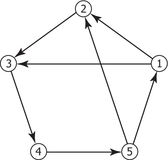
Example 2

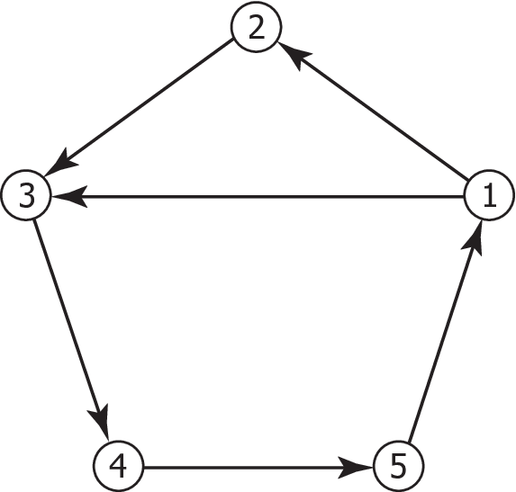
Consider the four digraphs reported in Fig. 7.

•

With the digraph in Fig. 7(a), we have that system (9) is asymptotically stable for $s\in(1/\cos(16\pi/5),\,1)$ (cf. Prop. 14). For $s=1/\cos(16\pi/5)$ , system (9) is marginally stable: at steady-state, its states oscillate with the same frequency and amplitude, and the phases are evenly spaced. For $s=1$ , average consensus is achieved (see the simulation results in Sect. 5.2).
•

With the digraph in Fig. 7(b), system (9) is asymptotically stable for $s\in(-1.6889,\,1)$ . For $s=-1.6889$ , system (9) is marginally stable. At steady-state, its states oscillate with the same frequency but have different amplitudes: the phases are regularly spaced. For $s=1$ , consensus (but not average consensus, since edge $(1,\,3)$ breaks the balancedness of the original five-vertex directed cycle), is achieved (see the simulation results in Sect. 5.2).
•

With the digraph in Fig. 7(c), we have the same qualitative behavior as with the digraph in Fig. 7(b). The only difference is represented by the stability threshold, that is now $s=-1.9441$ instead of $s=-1.6889$ .
•

With the digraph in Fig. 7(d), system (9) is asymptotically stable for $s\in(-1.3326,\,1)$ . For $s=-1.3326$ , system (9) is marginally stable and its non-oscillating states asymptotically converge to five different values. For $s=1$ , consensus (but, again, not average consensus) is achieved.

Note that we cannot leverage Prop. 12 to determine the stability interval of system (9) when it admits stable periodic solutions (the threshold values for the digraphs in Figs. 7(b) and 7(c), have been determined on a trial-and-error basis): however, Prop. 12 appears to provide the correct stability intervals in all the other cases (e.g., for the directed path in Fig. 6(a), or for the digraph in Fig. 7(d)). The analytical determination of the stability thresholds for general digraphs is the subject of on-going research. The directed graphs in Figs. 7(b) and 7(c) are particularly significative for showing the nontrivial connection existing between the topology of the digraph $\mathcal{D}$ and the threshold values: in fact, here, a single edge-orientation change $($ i.e., $(1,\,3)$ versus $(3,\,1))$ , yields two remarkably different thresholds: $s=-1.6889$ and $s=-1.9441$ . $\diamond$

5 Simulation results

Numerical simulations have been performed in order to illustrate the theory presented in Sect. 3 and Sect. 4.2. Sect. 5.1 deals with the case of undirected graphs, and Sect. 5.2 with the case of directed graphs.

5.1 Undirected communication graph

Consider a team of $n$ single-integrator agents,

\dot{{\mathbf{p}}}_{i}(t)=\,\boldsymbol{\nu}_{i}(t),\;\;i\in\{1,\ldots,n\},

where ${\mathbf{p}}_{i}(t)=[p_{ix}(t),\,p_{iy}(t)]^{T}\in\mathop{{\rm I}\mskip-4.0mu{\rm R}}\nolimits^{2}$ and $\boldsymbol{\nu}_{i}(t)\in\mathop{{\rm I}\mskip-4.0mu{\rm R}}\nolimits^{2}$ denote respectively the position and the input of vehicle $i$ at time $t$ . Let the control input of agent $i$ be of the form,

\boldsymbol{\nu}_{i}(t)\,=\,(s^{2}-1)\,{\mathbf{p}}_{i}(t)\,+\,s\!\!\!\sum_{j\,\in\,\mathcal{N}(i)}\!({\mathbf{p}}_{j}(t)-s\,{\mathbf{p}}_{i}(t)),\vskip-2.84544pt

(12)

where $\mathcal{N}(i)$ denotes the set of vertices adjacent to vertex $i$ in the communication graph⁸⁸ 8 Note that we implicitly assume here that parameter $s$ is broadcast in real-time to all the agents by a supervisor, via a centralized transmitter.. Then, the collective dynamics of the group of vehicles adopting control (12), can be written as,

\dot{{\mathbf{p}}}(t)\,=\,(-\boldsymbol{\Delta}(s)\,\otimes\,{\mathbf{I}}_{2})\,{\mathbf{p}}(t),

where ${\mathbf{p}}=[{\mathbf{p}}_{1}^{T},\,\ldots,\,{\mathbf{p}}_{n}^{T}]^{T}\in\mathop{{\rm I}\mskip-4.0mu{\rm R}}\nolimits^{2n}$ and “ $\otimes$ ” denotes the Kronecker product.
Fig. 8(a) shows the trajectory of 8 vehicles implementing the control law (12), when the communication topology is the cycle graph $C_{8}$ (the vehicles are initially on the vertices of a regular octagon centered at the origin, and their position is marked with a circle in the figure). For the sake of illustration, in our simulation we selected the following switching signal (see Fig. 8(c)):

s(t)=\left\{\begin{array}[]{lcl}0&\,\text{for}&t\in[0,\,1)~\text{sec}.,\\ -1&\,\text{for}&t\in[1,\,8]~\text{sec}.\end{array}\right.

The time evolution of the $x$ -, $y$ -coordinates of the agents is reported in Fig. 8(b). As it is evident in Figs. 8(a) and 8(b), the vehicles first converge towards the origin by maintaining equal interdistances, and then the even and odd agents cluster in two distinct groups (recall Prop. 2).

5.2 Directed communication graph

A scenario similar to that described in Sect. 5.1 is considered in Fig. 9. In this case, 5 single-integrator agents implement the control law (12) and communicate using a directed graph. This leads to an overall closed-loop system of the form,

\dot{{\mathbf{p}}}(t)\,=\,(-\boldsymbol{\Delta}(\mathcal{D}(s))\,\otimes\,{\mathbf{I}}_{2})\,{\mathbf{p}}(t).

The results in Figs. 9(a)-(c), are relative to the digraph in Fig. 7(a), i.e., $\textsf{D}_{5}$ . Fig. 9(a) shows the trajectory of the 5 vehicles starting from the position ${\mathbf{p}}(0)=[-1.5,\,-3,\,2.5,\,0,\,-4,\,2.5,\,4,\,-3,\,1.5,\,3]^{T}$ . As shown in Fig. 9(d),

s(t)=\left\{\begin{array}[]{lll}1/\cos(16\pi/5)&\text{for}&t\in[0,\,50)~\text{sec}.,\\ 1&\text{for}&t\in[50,\,100]~\text{sec}.\end{array}\right.

Fig. 9(b) displays the time evolution of the $x$ -, $y$ -coordinates of the agents. From Figs. 9(a) and 9(b), we can see that the vehicles first move counterclockwise along a common elliptical trajectory with frequency $f(5)=\frac{1}{2\pi}\tan(16\pi/5)$ and phases $\phi_{i}(5)=\frac{2\pi(i-1)}{5\tan(16\pi/5)}$ , $i\in\{1,\ldots,5\}$ , and then rendezvous at the point,

\Big(\,\frac{1}{5}\sum_{i=1}^{5}p_{ix}(50),\;\;\frac{1}{5}\sum_{i=1}^{5}p_{iy}(50)\Big),

i.e., they achieve average consensus (recall Prop. 14).
Finally, the results in Figs. 9(d)-(f), are relative to the digraph in Fig. 7(b). Fig. 9(d) shows the trajectory of the agents with ${\mathbf{p}}(0)\!=\![-4,-3,2.5,0,-4.5,1,4,\!-3.25,\!-2,3]^{T}$ . In this case (see Fig. 9(f)), parameter $s$ evolves according to:

s(t)=\left\{\begin{array}[]{lll}-1.6889&\text{for}&t\in[0,\,50)~\text{sec}.,\\ 1&\text{for}&t\in[50,\,100]~\text{sec}.\end{array}\right.

From Figs. 9(d) and 9(e), we see that the vehicles first move counterclockwise on five closed orbits, and then rendezvous at a single point (recall item 2 in Example 2).
It is worth observing here that the two simple control instances described in this subsection, look promising building blocks for more sophisticated multi-agent tasks, such as, e.g., for containment control [JiFeEgBu_TAC08] or cooperative patrolling [PasqualettiFrBu_TRO12].

6 Conclusions and future work

In this paper we have presented a generalization of the standard consensus protocol, called deformed consensus protocol, and we have analyzed its stability properties in terms of the real parameter $s$ for some special families of undirected and directed graphs. Preliminary results for arbitrary graph topologies are also provided: however, some work still needs to be done in order to precisely characterize in graph-theoretical terms, the variegated behavior of the deformed consensus protocol (a glimpse of such a richness of behaviors is provided by Examples 1 and 2). The proposed theory has been illustrated via extensive numerical simulations and examples.

In future works, we aim at studying the properties of the deformed consensus protocol when the (weighted) communication graph is not fixed but changes over time, at establishing a link with the existing cluster synchronization and group consensus literature [YuWa_SCL10, XiaCa_AUTO11], and at investigating other “parametric” Laplacian matrices besides the deformed Laplacian (a first step towards this direction has been recently done in [Morbidi_TAC13]).

References

[2] [] Altafini, C. (2012). Dynamics of Opinion Forming in Structurally Balanced Social Networks. PLoS ONE 7(6), e38135.
[4] [] Altafini, C. (2013). Consensus problems on networks with antagonistic interactions. IEEE Trans. Automat. Contr. 58(4), 935–946.
[6] [] Bauso, D., L. Giarré and R. Pesenti (2006). Nonlinear protocols for optimal distributed consensus in networks of dynamic agents. Syst. Contr. Lett. 55(11), 918–928.
[8] [] Brouwer, A.E. and W.H. Haemers (2012). Spectra of graphs. Universitext. Springer.
[10] [] Bullo, F., J. Cortés and S. Martínez (2009). Distributed Control of Robotic Networks. Applied Mathematics Series. Princeton University Press.
[12] [] Chen, F., Y. Cao and W. Ren (2012). Distributed average tracking of multiple time-varying reference signals with bounded derivatives. IEEE Trans. Automat. Contr. 57(12), 3169–3174.
[14] [] Cortés, J. (2008). Distributed algorithms for reaching consensus on general functions. Automatica 44(3), 726–737.
[16] [] Cvetković, D. and S.K. Simić (2009). Towards a spectral theory of graphs based on the signless Laplacian, I. Publ. Inst. Math. Beograd (NS) 85(99), 19–33.
[18] [] Cvetković, D. and S.K. Simić (2010). Towards a spectral theory of graphs based on the signless Laplacian, III. Appl. Anal. Discret. Math. 4(1), 156–166.
[20] [] Cvetković, D., P. Rowlinson and S.K. Simić (2007). Signless Laplacians of finite graphs. Linear Algebra Appl. 423, 155–171.
[22] [] Davis, P.J. (1994). Circulant Matrices. 2nd ed.. New York, Chelsea.
[24] [] de Abreu, N.M.M. (2007). Old and new results on algebraic connectivity of graphs. Linear Algebra Appl. 423(1), 53–73.
[26] [] Demmel, J.W. (1997). Applied numerical linear algebra. SIAM.
[28] [] Fagiolini, A., E.M. Visibelli and A. Bicchi (2008). Logical consensus for distributed network agreement. In: Proc. 47th IEEE Conf. Dec. Contr. pp. 5250–5255.
[30] [] Fagnani, F. and S. Zampieri (2008). Randomized consensus algorithms over large scale networks. IEEE J. Sel. Area Comm. 26(4), 634–649.
[32] [] Frasca, P., R. Carli, F. Fagnani and S. Zampieri (2009). Average consensus on networks with quantized communication. Int. J. Robust Nonlin. Contr. 19(16), 1787–1816.
[34] [] Godsil, C. and G. Royle (2001). Algebraic graph theory. Springer.
[36] [] Gohberg, I., P. Lancaster and L. Rodman (2009). Matrix polynomials. Vol. 58. SIAM, Philadelphia.
[38] [] Golub, G.H. and C.F. van Loan (1996). Matrix Computations. 3rd ed.. The Johns Hopkins University Press.
[40] [] Hislop, P.D. and I.M. Sigal (1996). Introduction to Spectral Theory: With Applications to Schrödinger Operators. number 113 In: Applied Mathematical Sciences. Springer.
[42] [] Jadbabaie, A., J. Lin and A.S. Morse (2003). Coordination of groups of mobile autonomous agents using nearest neighbor rules. IEEE Trans. Automat. Contr. 48(6), 988–1001.
[44] [] Ji, M., G. Ferrari-Trecate, M. Egerstedt and A. Buffa (2008). Containment Control in Mobile Networks. IEEE Trans. Automat. Contr. 53(8), 1972–1975.
[46] [] Kar, S. and J.Moura (2009). Distributed Consensus Algorithms in Sensor Networks with Imperfect Communication: Link Failures and Channel Noise. IEEE Trans. Signal Proces. 57(1), 355–369.
[48] [] Kibangou, A.Y. (2012). Graph Laplacian based matrix design for finite-time distributed average consensus. In: Proc. American Contr. Conf. pp. 1901–1906.
[50] [] Kumar, V., D. Rus and G.S. Sukhatme (2008). Networked Robots. In: Handbook of Robotics (B. Siciliano and O. Khatib, Eds.). Chap. 41, pp. 943–958. Springer.
[52] [] Mesbahi, M. and M. Egerstedt (2010). Graph Theoretic Methods in Multiagent Networks. Applied Mathematics Series. Princeton University Press.
[54] [] Milutinović, D. and P. Lima (2006). Modeling and Optimal Centralized Control of a Large-Size Robotic Population. IEEE Trans. Robot. 22(6), 1280–1285.
[56] [] Mohar, B. (1991). The Laplacian Spectrum of Graphs. In: Graph Theory, Combinatorics, and Algorithms (Y. Alavi, G. Chartrand, O.R. Oellermann and A.J. Schwenk, Eds.). Vol. 2. pp. 871–898. Wiley.
[58] [] Morbidi, F. (2012). On the Properties of the Deformed Consensus Protocol. In: Proc. 51st IEEE Conf. Dec. Contr. pp. 812–817.
[60] [] Morbidi, F. (2013, submitted). The Laplacian Pencil and its Application to Consensus Theory. IEEE Trans. Automat. Contr.
[62] [] Moreau, L. (2005). Stability of multiagent systems with time-dependent communication links. IEEE Trans. Automat. Contr. 50(2), 169–182.
[64] [] Olfati-Saber, R. and R.M. Murray (2004). Consensus problems in networks of agents with switching topology and time-delays. IEEE Trans. Automat. Contr. 49(9), 1520–1533.
[66] [] Olfati-Saber, R., J.A. Fax and R.M. Murray (2007). Consensus and Cooperation in Networked Multi-Agent Systems. Proc. of IEEE 95(1), 215–233.
[68] [] Pasqualetti, F., A. Franchi and F. Bullo (2012). On cooperative patrolling: optimal trajectories, complexity analysis, and approximation algorithms. IEEE Trans. Robot. 28(3), 592–606.
[70] [] Pasqualetti, F., D. Borra and F. Bullo (2013, submitted). Consensus Networks over Finite Fields. Automatica.
[72] [] Porfiri, M. and D.J. Stilwell (2007). Consensus Seeking Over Random Weighted Directed Graphs. IEEE Trans. Automat. Contr. 52(9), 1767–1773.
[74] [] Ren, W. and R.W. Beard (2005). Consensus seeking in multiagent systems under dynamically changing interaction topologies. IEEE Trans. Automat. Contr. 50(5), 655–661.
[76] [] Ren, W., R.W. Beard and E.M. Atkins (2007). Information consensus in multivehicle cooperative control. IEEE Contr. Syst. Mag. 27(2), 71–82.
[78] [] Spanos, D.P., R. Olfati-Saber and R.M. Murray (2005). Dynamic average consensus for mobile networks. In: Proc. 16th IFAC World Cong.. pp. 2893–2898.
[80] [] Strogatz, S.H. (1994). Nonlinear Dynamics and Chaos: With Applications to Physics, Biology, Chemistry, and Engineering. Studies in Nonlinearity. 1st ed.. Perseus Books Publishing.
[82] [] Tahbaz-Salehi, A. and A. Jadbabaie (2008). A Necessary and Sufficient Condition for Consensus Over Random Networks. IEEE Trans. Automat. Contr. 53(3), 791–795.
[84] [] Tisseur, F. and K. Meerbergen (2001). The Quadratic Eigenvalue Problem. SIAM Rev. 43(1), 235–286.
[86] [] Tsitsiklis, J. (1984). Problems in decentralized decision making and computation. PhD thesis. EECS Department, MIT.
[88] [] Wang, L. and F. Xiao (2010). Finite-Time Consensus Problems for Networks of Dynamic Agents. IEEE Trans. Automat. Contr. 55(4), 950–955.
[90] [] Xia, W. and M. Cao (2011). Clustering in diffusively coupled networks. Automatica 47(11), 2395–2405.
[92] [] Yang, P., R.A. Freeman and K.M. Lynch (2008). Multi-Agent Coordination by Decentralized Estimation and Control. IEEE Trans. Automat. Contr. 53(11), 2480–2496.
[94] [] Yu, J. and L. Wang (2010). Group consensus in multi-agent systems with switching topologies and communication delays. Syst. Contr. Lett. 59(6), 340–348.
[96] [] Zampieri, S. (2008). Trends in Networked Control Systems. In: Proc. 17th IFAC World Congress. pp. 2886–2894.

The Deformed Consensus Protocol Extended Version