Quantum Corrections to Thermopower and Conductivity in Graphene
Abstract
The quantum corrections to the conductivity and the thermopower in monolayer graphene are studied. We use the recursive Green’s function method to calculate numerically the conductivity and the thermopower of graphene. We then analyze these weak localization corrections by fitting with the analytical theory as function of the impurity parameters and the gate potential. As a result of the quantum corrections to the thermopower, we find large magnetothermopower which is shown to provide a very sensitive measure of the size and strength of the impurities. We compare these analytical and numerical results with existing experimental measurements of magnetoconductance of single layer graphene and find that the average size and strength of the impurities in these samples can thereby be determined. We suggest favorable parameter ranges for future measurements of the magnetothermopower.
pacs
65.80.Ck, 72.20.Pa, 73.22.PrI Introduction
Since its synthesis, graphene[1] has attracted a lot of attention, both for its novel electronic properties and its possible applications. One of the most remarkable aspects is that the weak localization effect, which is a typical low-temperature phenomenon due to quantum corrections to the conductivity , can in graphene be observed up to a temperature range of 200 Kelvin.[2, 3] It has been theoretically predicted that the sign of these corrections strongly depends on the kind of impurities in the graphene sample,[4] so that both positive and negative magnetoconductivity, the so-called weak antilocalization effect, can be observed. This effect is well known to occur due to spin-orbit interaction, even though the latter is typically very weak in graphene. Noting that the graphene lattice is composed of two sublattices, one can formulate the sublattice degree of freedom as an isospin which is strongly coupled to the momentum. Thereby, any elastic scattering that breaks the graphene sublattice symmetry is expected to result in weak antilocalization. This is made more complicated, however, by the fact that there is another discrete degree of freedom in graphene, the two degenerate Dirac cones, which can correspondingly be formulated by introducing a pseudospin index. Accordingly, any scattering which mixes these two valleys can result in yet another change of the sign of the quantum correction to the conductivity, and thereby to the restoration of weak localization. More recently, thermopower in graphene has been measured by several groups.[5, 6, 7, 8] The classical thermopower of graphene has been calculated with a range of different methods. The experiments show good agreement with the Mott formula, which corresponds to the leading term of the Sommerfeld expansion at low temperatures and large gate voltages.[9] Close to the Dirac point, thermopower shows an unusual behavior, being linear in gate voltage, and changing sign. Thus, while usually thermopower is expected to increase as the Fermi energy, the electron density and thereby the conductivity are lowered, in graphene the thermopower becomes smaller as the Dirac point is approached and the electron density and the conductivity are reduced.
The main aims of this paper are, firstly, to find out if there are sizable quantum corrections to the thermopower in graphene and whether they are sensitive to weak magnetic fields, secondly, to present and analyze the combined analytical and numerical theory in order to provide the basis for a more quantitative analysis of experimental results on magnetoconductance of graphene. This will allow one to characterize samples, in particular the density, strength, and size of carrier scatterers, more accurately.
We restrict our attention to the diffusion term of the thermopower and do not consider the phonon drag contribution, which becomes relevant only at high temperatures. In normal metals, the quantum corrections to the diffusion thermopower are known to be dominated by the weak localization corrections to the conductivity, yielding . [10, 11, 12] Thus, when the conductivity is reduced by the weak localization correction, the thermopower becomes enhanced. This is expected since the thermopower is known to increase from a metal towards an insulator. Because of the particular electronic properties of graphene, where the sign of the quantum correction can change upon varying the gate voltage, it could be expected that these quantum corrections to thermopower are particularly large in graphene. We therefore determine the strength and the sign of the resulting magnetothermopower and analyze in detail how it changes with impurity parameters such as range, density, and strength and with the gate voltage.
This paper is organized as follows. We start in Sec. II with a short introduction to the electronic properties of graphene. We introduce the model for the description of the impurity potential in Sec. III and list the resulting momentum scattering rates and their dependence on the impurity matrix elements. In Sec. IV.1 we give a brief review of transport theory, in particular the theory of weak localization corrections to the conductivity and its application to graphene. In Sec. IV.2 we review the theory of thermopower and address leading quantum corrections.
In Sec. V we present a numerical method to calculate the conductance which is based on the recursive Green’s function technique (Sec.V.2). We introduce the Hamiltonian that models impurities in graphene for the numerical calculation in Sec. V.3 and relate it in Sec. VI to the impurity model introduced in Sec. III. This connection makes it possible to display the related transport scattering rates from Sec. III and Sec. IV as functions of the sample parameter of the numerical method, Sec. V, which is done in Sec. VI.2.
In Sec. VII we present the numerical results for the conductance, Sec.VII.1, and thermopower, Sec.VII.2. In Sec. VIII we analyze the numerical results by fitting them to the analytical results in Sec. VIII.1. In Sec. VIII.2 we attempt an ab initio analysis. To this end, we use the relation of the scattering rates to the impurity parameters of the numerical calculations and insert it in the analytical formulas given in Sec. IV. In Sec. VIII.3 we present the analytical results for the quantum corrections to the conductance at zero magnetic field. In Sec. VIII.4 we present the results for the quantum corrections to the thermopower at zero magnetic field and the resulting magnetic field dependence of the thermopower. In Sec. IX we compare the numerical and the analytical results with experimental results on weak localization corrections to the conductance. Finally, we draw the conclusions and summarize our results in Sec. X. In appendix A the Hamiltonian is given in matrix notation. In appendix B we present analytical results for the magnetoconductance when the warping rate is neglected, .
II Electronic Structure of graphene
Let us start with a brief review of the electronic properties of graphene, introducing the notation used in this article. We follow the convention of McCann and coworkers.[4] For an overview and comparison of notations, see also 13, 14, 15 and 16
Graphene is a two-dimensional layer of carbon atoms arranged in a honeycomb lattice. These carbon atoms are connected by strong -bonds with their three neighboring atoms. The corresponding energy bands are filled valence bonds, lying deep below the Fermi energy. The -bond leads to the formation of a band which is exactly half filled in ungated and undoped graphene. Thus, to study transport properties we can restrict the model to this -band. The basis of the Bravais lattice consists of two atoms, each one of them forming one sublattice, named A- and B-sublattice.
The electronic band structure shows two degenerate half filled cones, which in momentum space are located on the sites of the hexagonal reciprocal lattice. Close to zero energy, the Dirac points, the dispersion is in good approximation linear. Each Dirac cone is part of a sublattice, the K- and K’-valleys.
Accordingly, the Hamiltonian can be written as a -matrix which, close to the Dirac points in linear approximation, becomes
| (1) |
where is the diagonal Pauli matrix in K-K’ space, and are components of the momentum in the plane, and
| (2) |
with the non-diagonal Pauli matrices in the sublattice (A,B)-space. The next correction term to the dispersion is quadratic and given by
| (3) |
where is the parameter of warping, which is given by[17, 18]
| (4) |
In this notation the 4-component Bloch-states are given by
| (5) |
The Hamiltonian can be more compactly written in the isospin and pseudospin notation, which is particularly convenient for the purpose of understanding the sign of weak localization corrections to the conductivity. Following the definition of McCann and coauthors,[4] we set
| (6) | |||||
| (7) |
and
| (8) | |||||
| (9) |
where , are the Pauli matrices and
the identity matrix in the sublattice (A,B)-space, and ,
are the Pauli matrices and the identity matrix
in K-K’ space. The vector of the matrices is the isospin vector referring to
the sublattice (A,B) degrees of freedom, and is the pseudospin vector
referring to the valley (K, K’) degrees of freedom.
In this notation
the Hamiltonian can be written as
| (10) |
Note that is independent of the pseudospin , while the warping term breaks the pseudospin symmetry.
III Impurities in graphene
Disorder can have many different origins in graphene such as adatoms and vacancies, while substitutional defects are rather unlikely due to the strength of the -bonding. For the purpose of the transport calculations, it is rather convenient to classify the disorder according to whether it breaks the isospin symmetry (A, B sublattices) or the the pseudospin symmetry (K, K’ valleys). Thus, the Hamiltonian of nonmagnetic disorder has in the representation of the pseudospin and the isospin the general form,[4]
| (11) |
where is the identity matrix. is the part of the disorder potential which leaves both the isospin and the pseudospin symmetry invariant, while the other terms are breaking either of these symmetries with the amplitudes . We note that this disorder Hamiltonian is invariant under time reversal, and and thus indeed describes nonmagnetic disorder. See Appendix A for the explicit matrix representation of the Hamiltonian.
The corresponding scattering rates in Born approximation are given by
| (12) |
where is the density of states per spin and valley. We can thus define the total scattering rate as
| (13) |
The intervalley scattering rate is obtained by summing over all matrix elements which couple to the transverse pseudo spin components and , yielding
| (14) |
where we introduced to denote the transverse components, noting that and since and .
The intravalley scattering rate is accordingly given by
| (15) |
The trigonal warping term in the kinetic energy of graphene results in an asymmetry of the dispersion at each valley with respect to momentum inversion,[19] while the total Hamiltonian including both valleys preserves that symmetry. Therefore, the pseudospin is expected to precess in the presence of the warping term. In the presence of elastic scattering the pseudospin channels are expected to relax accordingly, as in motional narrowing, in proportion to the scattering time ,
| (16) |
IV Transport Theory
IV.1 Weak Localization Corrections to the Conductance in Graphene
Quantum corrections to the conductance, the so-called weak localization corrections, originate from the quantum interference of electrons propagating through the sample. On time scales exceeding the elastic mean free time , electrons move diffusively and their return probability can be enhanced due to the constructive interference of the amplitudes for propagation on closed diffusion paths, as long as that time does not exceed the phase coherence time . In the presence of spin-orbit interaction, the spin precesses as the electron moves on closed paths, and the phase of the amplitudes for clockwise and anticlockwise propagation no longer match, unless the total spin of these two propagations adds up to zero. This spin singlet channel leads to destructive interference, and thereby an enhancement of the conductance, the weak antilocalization correction.
Since the spin-orbit interaction in graphene is weak, in the absence of magnetic impurities, there are two independent spin channels in graphene and the quantum corrections are doubled due to this spin degeneracy. However, since the electron momentum is directly coupled to the isospin (due to the A-B sublattice degree of freedom) in the electron Hamiltonian of Eq. (10), any momentum scattering will result in the breaking of the isospin symmetry. Therefore, there is a finite contribution from the interference of two closed electron paths whose total isospin is zero, leading to weak antilocalization in the isospin singlet channel.
Let us now consider the influence of the pseudospin degree of freedom of the two valleys in graphene on the weak localization corrections. Formulating the conductance corrections in the representation of pseudospin singlet and triplet modes, one has, in two dimensions, [4]
| (17) |
where is the diffusion constant, which in graphene is related to the elastic scattering time as , and the momentum integral has an upper cutoff , where is the elastic mean free path. The superscript corresponds to the pseudospin and the subscript to the isospin.
Without magnetic field () the Cooperon modes are given by
| (18) |
Here, is the dephasing rate caused by electron-electron and electron-phonon interactions, which provides the low-energy cutoff of the diffusion pole of Eq. (18). The elastic scattering from impurities can break the pseudospin symmetry and results in the following pseudospin relaxation rates,
| (19) | |||||
| (20) | |||||
| (21) |
where
| (22) |
We note that Thus, the pseudospin triplet Cooperon modes are attenuated. Performing the integral over momentum one thus obtains logarithmic weak localization corrections at ,
| (23) |
where
| (24) | |||||
and . The dependence of the various scattering rates [Eqs.(14), (15) and (16)] on the impurity potential amplitudes is given by Eq. (12). One can see that both the sign and the amplitude of the weak localization corrections depend strongly on the impurity type.
As we will study in detail below, impurities with large correlation lengths mix valleys weakly, , and therefore only attenuate two of the pseudospin triplet modes, in a similar way as the relaxation rate due to the warping term of Eq. (16). This effect leads to the vanishing of the weak localization effect and a flat magnetoconductance.
Upon applying an external magnetic field, the weak localization corrections are suppressed. Solving the Cooperon equation in the presence of a magnetic field by summing over the Landau levels, one finds that is given by
| (25) |
where the function in Eq. (25) is given by
| (26) |
where is the Digamma function and the magnetic rate is
| (27) |
For weak magnetic fields, one can use the simplified form[4]
| (28) |
Equation (25) can be expanded for small magnetic fields, yielding
| (29) |
where
| (30) | |||||
In Fig. 1 we plot the curve obtained from the solution of as function of the parameters and . This curve separates the region of positive and negative magnetoconductance. We note that this separation line does not coincide with the curve , which corresponds to the vanishing of the weak localization correction and separates the parameter space regions of weak localization and weak antilocalization (corresponding to negative and positive quantum corrections to the conductivity at , respectively). As seen in Eq. (23) the latter separation line depends on an additional parameter, the total scattering rate .

IV.2 Thermopower
Applying a thermal gradient to a metallic sample induces not only a thermal current but also an electrical current density , where is an applied electric field and is the chemical potential. Here, denotes the thermoelectric coefficient. Under open circuit conditions, the thermal gradient results in a finite voltage proportional to the temperature difference , where the proportionality constant is the thermopower: . At low temperatures, the thermopower is dominated by the diffusion of the electrons in the sample and the phonon drag contribution becomes small. Expanding in the ratio of temperature to Fermi energy and keeping the leading term, one arrives at the Mott formula, which relates the thermopower to the derivative of the conductivity with respect to the Fermi energy,
| (31) |
This formula is valid for low temperatures, and
large chemical potential. For , which is the case in this paper,
the chemical potential is equal to the Fermi energy.
Here, is the negative electron
charge. Thus, when the carriers have negative charge, thermopower is
expected to be negative, while for holes it becomes positive. We note
that the elemental unit of thermopower is given by a ratio of
natural constants .
Furthermore this formula is valid not only classically but also includes quantum corrections through the conductivity. Thus, expanding in the quantum correction to the conductivity , we can write the leading quantum corrections to the thermopower, , as
| (32) |
This relation is also supported by direct diagrammatic calculations of quantum corrections.[10, 11, 12] In standard metals, the last term on the r.h.s of Eq. (32) is small and the thermopower is dominated by the quantum correction to the conductivity. In this work we revisit this relation to find out whether this also holds for graphene, or whether the second term in Eq. (32) is sizable.
V The recursive Green’s function method
In this section we introduce the numerical method used to calculate the electrical conductivity and the thermopower. We employ the recursive Green’s function method,[20, 21], which has been previously applied to graphene in Refs. [22, 23, 24, 25]. Below, we begin by reviewing the essential elements of this method.
The graphene sample is assumed to be connected to two semi-infinite leads which are modeled by a square lattice. When contacting the leads at the zigzag edges of the graphene sample, there is no wave function mismatch between the propagating modes in the square lattice leads and the graphene sample, provided that a proper energy shift is used.[26] The graphene sample is sliced transversely into equal cells, with each cell containing sites. We study the transport as function of by changing the length of the sample, and as function of by changing the sample width . When the free edges are of the armchair type, the sample dimensions are related to to and by and , where is the lattice constant set as the distance between two atoms of the same sublattice. See Fig. 2 .
V.1 The conductivity
In two dimensions, the electrical conductivity is related to the conductance by the standard expression and thus can be expressed in terms of retarded Green’s function through the Caroli formula
| (33) |
where denotes the advanced/retarded Green’s function connecting two opposite contact regions (right and left). Here, denotes the trace over transverse sites at the lead-sample interface. The matrix elements of the level width matrix can be expressed in term of the transverse wave functions of the lead propagating modes,
| (34) |
Here, the sum runs over the propagation modes and is the longitudinal propagation velocity. Next we describe the method used to obtain the Green’s functions of the sample.
V.2 The Green’s function
In order to obtain the Green’s function amplitude between sites at the contacts , we start with the surface Green’ function of one of the contacts, which is presumed to be known. Then we add one slice of transverse sites , and calculate the Green’s function from the contact up to that slice. We repeat the procedure, adding slice by slice, until the end of the sample is reached. This procedure is done from left to right, and then in the opposite direction in order to calculate the full Green’s function of the system. The slicing is displayed in Fig. 2.

Each line in Fig. 2 represents a hopping amplitude from one sublattice to another. This is described by the hopping matrix . This matrix, together with the Green’s function of every new single slice and the Green’s function that includes the contacts and the sample up to slice , defining , are inserted in the Dyson equation to obtain the new . One can easily understand that the speed of the procedure strongly depends on the slicing scheme adopted. In general, more slices mean more steps to calculate, but each slice consists of fewer atom sites and so its calculation is done faster since an inversion at each slice is required. The complexity of the calculation scales as .
The Green’s function of the contacts has been derived previously and is given by [27]
| (35) |
with
| (36) |
where represents the modes of the transverse wave function and is the hopping rate in -direction. We can transform from the channel representation into in the site representation by
| (37) |
with the transverse wave functions given by
| (38) |
V.3 Inclusion of impurities
We now look at the model disorder used in the numerical calculations. The sites of the graphene sample are occupied by uniformly randomly distributed Gaussian scatterers with a random potential . We can write for the overall potential resulting from all scatterers at the points as
| (39) |
Here, is the range of the potential and are the lattice sites. The concentration of scatterers is given by , where is the total number of lattice sites. We focus on pairwise uncorrelated impurities, , each vanishing on average, .
We use as an input parameter the dimensionless correlation strength , which is defined by the equation for the impurity potential correlation function as
| (40) |
In the limit of dilute impurities, summing over all sites yields
| (41) |
Inserting Eq. (39) into Eq. (41) and using the relations
| (42) |
we get[28]
| (43) |
where is the half width of the box distribution of the amplitude of the Gaussian imputities , defined in Eq. (39), and
| (44) |
Thus, the parameter depends on , , and and is proportional to concentration of impurities . It is useful to introduce the typical impurity strength amplitude , which is related to and by
| (45) |
VI Connection between the two impurity descriptions from section (III) and (V.3)
VI.1 Impurity potential
In this subsection, we establish the link between the description of the impurities in graphene in the pseudospin and isospin representation, as introduced in Sec. III, and the Gaussian impurities introduced in the previous section.[13, 28] McCann and coworkers assume that the different components of the impurity potential Eq. (11) are uncorrelated,
| (46) |
where denote the pseudospin and isospin indices as introduced in Eq. (11). We can decompose the potential due to one impurity at a given site of the lattice, , in Fourier components. Defining the vector connecting sublattices as , we find for the Fourier component of on sublattice A [13, 29]
| (47) |
and for sublattice B
| (48) |
where the sum is over all elementary cells. We assume and to be slow functions of the momentum . Thus, the quantity is proportional to the first-order scattering amplitude for electrons on the same sublattice where the impurity resides, while is the one for electrons on the other sublattice. We will explicitly consider two values: the intravalley scattering, , and the intervalley scattering, , where connects the two different valleys in the reciprocal space and has the amplitude . We thus have and for intravalley scattering in K-K’ space and and for intervalley scattering. Intravalley scattering means that the electron that is scattered does not leave the original cone-shaped valley in k-space, while in the intervalley scattering process the electron starts in the K valley and ends after scattering in the K’ valley or viceversa.
Equations (47) (48) can now be displayed in the form of Eq. (11) using a matrix notation. For impurities located on sublattice A in the elementary cell and small , we can approximate
| (75) | |||||
and, equivalently, for impurities in sublattice B,
| (102) | |||||
where we used the fact that vanishes due to the symmetry of graphene (otherwise we would not have any zeros in the secondary diagonal, but terms involving ).
As the next step, we convert Eq. (75) and Eq. (102) into one single impurity potential matrix that can be compared with Eq. (11). This is done by calculating the autocorrelation function , with , set by
| (103) |
where the averaging is with respect to the positions of the impurities and the impurity strength , whereas the averaging is only with respect to . The normalization factors are already included in the prefactor of the r.h.s. of Eq. (103).
Comparison of Eq. (103) with the matrix notation of the impurity as introduced in Eq. (11) leads, with the help of Eq. (45) and the use of the impurity position averaged parameter from Eq. (44), to the following set of equations
| (104) | |||||
| (105) | |||||
where
| (206) | |||||
Note that is a measure of the total impurity strength averaged over all impurities. Since is proportional to their concentration , increases with as
. In the limit of short-range impurities, , we find
while for long-range impurities, , we find
| (258) | |||||
In that limit, Eq. (VI.1), only is not zero. We can see here that, due to symmetry, is always and we are left with only one parameter . This is shown in Fig. 3. Also displayed are the potential terms , and which, as we have seen above, are proportional to the impurity scattering matrix elements , , and .
Within the simplified picture of this subsection, the last result is again consistent with short-range scatterers mixing valleys and sublattices while long-range scatterers mixing only sublattices.


VI.2 Scattering rates
We now calculate the scattering rates of Eq. (14) and Eq. (15) and combine them with the potential Fourier components of Eqs. (104), (105), and (VI.1). ( Note: We restrict us here to the Born approximation. Going beyond that approximation, one needs to include all multiple impurity scattering, which yields corrections which depend logarithmically on energy[14], and can yield according to Mott’s law additional contributions to thermopower.) The density of state per spin and per valley , which is given by
| (276) |
is inserted into the general expression for the scattering rate, Eq. (12), where
| (277) |
and is the area of the primitive
unit cell.
In case of Gaussian scatterers of Eqs. (104), (105), (VI.1), and Eqs. (75) and Eq. (102), only the main- and off-diagonal matrix elements of Eq. (11) are non zero. This helps us simplify Eqs. (14) and (15), so that we find
| (278) |
resulting in
| (279) | |||||
| (280) |
Inserting Eqs. (104), (105), and (VI.1) and by using Eqs. (12) and (16) leads to
| (281) | |||||
| (282) | |||||
| (283) |
Now, using Eq. (276) we find
| (284) | |||||
| (285) | |||||
| (286) | |||||
| (287) |
Since the dephasing rate in the numerical calculations, the low-energy cutoff is provided by the Thouless energy[30]
| (288) |
where is the length or width of the sample, depending which one is smaller, , if we have , for , and D is the diffusion constant given by[31]
| (289) |
Thus, we get the following ratios:
| (290) | |||||
| (291) | |||||
| (292) |
Since the factors , (, and , depend on the impurity parameters and , as shown in Fig. 3, by tuning one of these parameters and the system size , and Fermi energy , one cam move in the - diagram of Fig. (1). This phase diagram is equivalent to what has been shown in the experimental paper,[3] where the temperature has been varied to reach the different regions of the diagram. By tuning these parameters, a change from weak localization to weak antilocalization can be observed. We note that a change of the impurity concentration changes and , while the ratio originating from the warping rate is independent of the impurity concentration .
For the magnetic rate we find accordingly,
| (293) |
VII Numerical Results


All results presented in the following are for samples with armchair edges. Most calculations have also been done with zig zag edges, especially in the case of small systems, but they do not show any significant difference and are consequently not displayed here. We consider always samples with an aspect ratio of 1, , ranging from and ; , , up to , . The correlation length is given in units of , the lattice constant. The correlated disorder strength is the dimensionless parameter, defined in Eq. (43). For small systems, we use and , while for the larger system, we consider only , . Unless explicitly mentioned otherwise, the impurity density is set to , meaning that of the atomic sites are occupied by impurities. The experiments on weak antilocalization[3] indicate indeed that this is a realistic concentration of impurities in these graphene samples. We also performed the calculations for higher densities up to .
Impurities are uniformly distributed across the sample. For each impurity realization we calculate the electrical conductivity as delineated above. We run the numerical calculations for different realizations in order to average the results for the conductivity and thermopower. For the larger systems, turns out to be sufficient, since self-averaging improves with increasing system size. The Fermi energy, is displayed in units of the hopping parameter , which is set to eV. We consider the range , where corresponds to the Dirac point. The magnetic field is displayed as the magnetic flux through the whole sample in units of the magnetic flux quantum .


VII.1 Conductivity
VII.1.1 Magnetoconductance sign
Numerical results for the magnetoconductivity are displayed in Fig. 4. We can distinguish the weak localization from the weak antilocalization by the sign of the magnetoconductance:
| (294) |
Negative magneto conductance at weak magnetic fields corresponds to weak antilocalization, since the magnetic field reduces the quantum correction and thereby the conductance. Positive magneto conductance corresponds to weak localization. As seen in Figs. 5, this sign can change at large magnetic fields. This occurs as soon as the magnetic rate exceeds all symmetry breaking rates defined in Eq. (12). We note that the two-dimensional samples considered in the numerical calculations are rather small, with length and width that are much smaller than the magnetic length for moderate magnetic fields (). Therefore, the sensitivity of the conductivity to an external magnetic field is reduced and the magnetic rate becomes suppressed for to[32]
| (295) |
where is a geometrical factor of order unity. On the other hand, the symmetry breaking rates , Eq. (12) do not depend on the system dimensions and . Only the relaxation rate originating from the warping term, , acquires a small sample size dependence and becomes smaller when . Therefore, as seen in Fig. 4, the change of the weak localization corrections occurs only when the magnetic fluxes through the samples corresponds to huge magnetic fields. This is due to the small samples considered in the numerical calculations.
As seen in Fig. 4(a), for small correlation length one observes positive magnetoconductance, while at a larger correlation lengths negative magnetoconductance occurs for the same impurity strength , see Fig. 4(b). As we will analyze in detail below, this can be explained by the reduction of the intervalley scattering amplitude with the increase of the correlation length , as shown in Fig. 3.
A transition between positive and negative magnetoconductance is observed as function of the Fermi energy , as seen in Fig. 4(c). Similar transitions can be observed when changing or , which we do not show here.
VII.1.2 Magnetoconductance amplitude
In addition to the sign of the magnetoconductance, the amplitude of the magnetoconductance is important and can reveal more information on the nature of the impurities in the sample. As a measure of the amplitude of the magnetoconductance, we take the difference between the conductance at the first extremum and the one at zero magnetic field (B=0),
| (296) |
Positive thus means that there is a weak localization dip at weak magnetic fields, while negative values correspond to the amplitude of the weak antilocalization peak. We summarize the different types of magnetoconductivity schematically in Fig. 6. The amplitude is indicated by arrows, both in the case when there is no sign change as the magnetic field is increased (1), as well as when the sign changes, (2). The quantum conductance corrections vanish at large magnetic fields, when is of the order of the elastic mean free path . This magnetic field we denote as , as defined by .

As seen in Fig. 4, there are still statistical fluctuations on smaller magnetic field scales, despite the large number of realizations , which we used in the averaging of the conductance.
VII.1.3 Phase diagrams
Magnetoconductance sign


In order to study the crossover between positive and negative magnetoconductance as function of the three impurity parameters , , and , we use Eq. (294) at weak magnetic fields to assign the value for negative magnetoconductance (NMC) and for the positive magnetoconductance (PMC). With this information we create three such sign phase diagrams, varying two parameters while the third parameter stays fixed. For better visualization, the diagrams are colored yellow for negative and red for positive magnetoconductance. The crossing line is highlighted by the black line. We note that the numerical data is given only at the crossings of grid lines. We used an interpolation method to get the continuous crossing line. As seen in the diagram, PMC occurs for short-range impurities with in the whole range of impurity strengths . This is expected since short-range impurities cause intervalley scattering and thereby suppress the pseudospin triplet Cooperons.
For impurities with larger correlation lengths (), NMC is observed for strong and large . Surprisingly, there is a regime at weak and small where PMC occurs even for large . We observed similar behavior for other sizes M and N which we do not display here. In the diagram we see a change from PMC to NMC when moving away from the Dirac point. At the Dirac point we observe a change at . For t only NMC is observed for . The phase diagram shows that for PMC occurs independent of the Fermi energy. At larger a change to NMC occurs, as expected.
In order to get a simpler representation of the results, we merge all three two-dimensional phase diagrams into one three-dimensional phase diagram, in which each of the parameters , and is represented by one axis, Fig.(8).

Magnetoconductance Amplitude
Using Eq. (296) we determine the amplitude of the magnetoconductance and plot it in contour plots in the , the and the plane, respectively, in Fig. 9. In these figures, the contour lines are tagged with the corresponding numbers calculated from Eq. (296). The main features already observed in the magnetoconductance sign phase diagrams can be seen in Fig. 9: PMC occurs for short-range impurities with irrespective of and . For impurities with larger correlation lengths (), there is NMC for strong and large , as expected. At weak and small , PMC occurs even for large . Its amplitude remains weak, however, corresponding to only a small weak localization dip at weak magnetic fields. This is displayed in Fig. 10.


VII.2 Thermopower


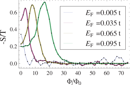


Next, we calculate the thermopower , as introduced in Sec. IV.2, using the Mott formula of Eq. (31) in order to see if there are quantum corrections and, as a result, magnetothermopower. To this end, we use the results for the conductance and its dependence on Fermi energy from the previous section to calculate and analyze and the thermopower . We note that by expanding in the quantum corrections of the conductivity to first order, we can write the quantum correction to the thermopower as
| (297) |
where . Since the conductance change with magnetic field is only of the order of , the first term in Eq. (297) is of order . Moreover, since vanishes at the Dirac point and increases linearly with the gate voltage, we expect the last term to become more important in the vicinity of the Dirac point. This is confirmed by the numerical results shown in Fig. 11(b) where is plotted as function of magnetic field. This quantity decays with magnetic field; the larger the Fermi energy , the larger is the sensitivity to the magnetic field. As shown in Fig. 11(a), the thermopower shows the same qualitative behavior, namely, a reduction of the amplitude of the thermopower when a magnetic field is applied. For positive gate voltage the thermopower is negative, so that we obtain positive magnetothermopower.
For the largest samples considered, we also observe an initial increase of at weak magnetic fields, and a peak which becomes enhanced with increasing Fermi energy (see Fig. 12), followed by a decay to its classical value at larger magnetic fields. Correspondingly, in these samples the amplitude of the thermopower (see Fig. 12(c)) first is enhanced when the magnetic field is applied and then it decreases toward its classical value at larger magnetic fields.
Since the magnetic field suppresses quantum corrections, we can obtain the classical value numerically from the high-magnetic field limit. Since the thermopower is fluctuating even in the range where it should saturate towards the classical limit, we needed to average over the fluctuations of the data points at different magnetic fields. For every set of parameters we thereby calculate and use as a definition for the quantum corrections the difference to the thermopower without magnetic field,
| (298) |
In the following, we explore the size and sign of these quantum corrections of the thermopower, and how they depend on the impurity parameters, such as the strength and the correlation length , and on the Fermi energy. In Fig. 13(a) we plot the values of as function of these three parameters. As we are particularly interested on how these quantum corrections to the thermopower are related to the weak localization corrections to the conductivity, we also plot the magnetoconductance amplitude (MCA) in Fig. 13(b) in units of . We notice that the set of parameters giving the most pronounced weak antilocalization seems also to yield the strongest thermopower enhancement. We will explain and analyze this effect in detail in Sec. VIII.4. This behaviour can also be seen when looking at the MC amplitude phase diagrams as function of in Fig. 9 since the derivative is the highest when there is a strong increase of values in the direction. This is the case in the regime of weak antilocalization, while a smaller change is observable in the weak localization regime, see Figs. 9(c) and 9(d).
VIII Analysis of Numerical Results
In order to get a better understanding of these numerical results for the magnetoconductance and the magnetothermopower, we compare them with the analytical expression of Eq. (25) and use the scattering rates and and the effective dephasing rate as fitting parameters. We also attempt an ab initio calculation where we use the input parameters of the numerical calculations to calculate directly the different scattering rates , insert these in the analytical expression, and compare the result with the numerical ones.
VIII.1 Fitting of the numerical results
For the fitting procedure, we picked the sample size and , where we observed a clear transition between weak antilocalization and weak localization when changing the parameters , and the Fermi energy, see Fig. 9. As mentioned before, since the magnetic length exceeds the system size in the magnetic flux range considered, we have to use the appropriate magnetic scattering rate , Eq. (295), which is strongly reduced by a geometrical factor compared to the two-dimension limit. As discussed above, since the numerical results are done at zero temperature, the dephasing rate can be substituted by the Thouless energy, see Eq. (288).
VIII.1.1 Fitting with a fixed
In this subsection, the two fitting parameters in Eq. (25) are taken to be and , while is calculated directly from Eq. (288). For the parameter range , and , we find that Eq. (25) fits well. Within this parameter region, we find the transition line between weak antilocalization and weak localization. We concentrate our fitting procedure to the validity range of the analytical formula at small magnetic flux, where , Eq. (295).


We show the results of the fitting exemplary for some parameters in Fig. 14(a), where the magnetoconductance is positive. In that case of pronounced weak localization, the fitting becomes worse, and the uncertainty in the set of and is larger.


For each parameter set used in the numerical calculations, we get a set of fitted values of the rates - which we plot in the diagrams of Figs. 15(a) and 15(b) as a symbol. The color of the symbols indicates the value of , while the symbol itself depends on the correlation length as shown in the legend. Weak localization corresponds to empty symbols and weak antilocalization to filled symbols. The range of scattering rates is and . Thus, the intervalley scattering rates are typically several magnitudes smaller than the intravalley scattering rates for the range of considered. The black line is obtained from in Eq. (30), indicating the transition between weak antilocalization and weak localization. With the exception of a few data points, we find good agreement. We can improve the agreement by fitting also as shown in the next section.
VIII.1.2 Fitting
We repeat the fitting procedure for the same sample but now taking as a third fitting parameter. We focus on the range of parameters , and . Close to the transition the extra fitting parameter does not change the result significantly. The result of the fitting procedure for some parameter values is displayed in Fig. 14(b) . As in Sec. VIII.1.1, we display the resulting , , and in a - diagram in Figs.15(c) and 15(d).
We find that the results fall in the range and . The agreement with the analytical results, the black solid line in Fig. 15, is improved. All numerical results fall on the expected side of the weak antilocalization to weak localization transition line.
VIII.2 Ab initio calculation
In this section we will attempt an ab initio calculation in the sense that we use the input parameters of the numerical calculations to calculate directly the different scattering rates , insert them into the analytical formula of Eq. (30) for the weak localization corrections, and compare the latter to the numerical results. For this calculation we choose the following parameter ranges. The impurity width is varied from to in steps of , the impurity strength V from to in steps of eV (corresponding to between approximately 0.05 and 2) and from to in steps of (note that the analytical result is not valid too close to the Dirac point ). The impurity concentration is set to as before, if not explicitly mentioned otherwise.
VIII.2.1 Conductance
Magnetoconductance sign transition
Using the explicit relations between the scattering rates and the parameters , , and , as derived in Sec. VI.2, in Fig. 16 we show a - diagram.

In Fig. 16 we display the magnetoconductance trajectories in the - plane by changing the impurity parameters and . For instance, this is done by changing for fixed and eV, red dots, and by changing and blue/green dots, respectively, for fixed and . The impurity concentration is kept fixed, its dependence inferred from Eqs. (290) and (291).
As expected, increasing the range of the impurities induces a change from weak localization to weak antilocalization, see the red arrow. When increasing the impurity strength one moves toward weak localization, see the blue arrow. Increasing the Fermi energy one also moves towards weak localization, see the green arrow. The diagram shows that saturates at fixed Fermi energy toward a lower limit since the ratio of the warping rate and the dephasing rate, converges to a finite value, Eq. (292), independently of and . At small correlation lengths () we find that the term dominates; a dependence on the strength of the impurities and a dependence on the Fermi energy emerge, in agreement with Eq. (291). In the regime of large correlation lengths (), we observe instead a dependence, which is in agreement with the dependence of the warping rate of Eq. (292). For comparison, we plot the - diagram without the warping term in Appendix B ( Fig. 26). Next, we transform Fig. 16 into the form of the phase diagram of Fig. 7(a). The resulting magnetoconductance sign diagram is shown in Fig. 17 for two different Fermi energies.


Magnetoconductance Amplitude


Having investigated the dependence of the sign of the magnetoconductivity, let us now study its amplitude using Eq. (296) to evaluate Eq. (25) with given by Eq. (26).

The resulting analytical magnetoconductance amplitude is shown in Figs. 18 and 19. In Fig. 18(a) the amplitude shown in Fig. 18(b) is displayed as function of and . Since the warping term dominates for large correlation lengths () and does not depend on and , regions I and II collapse onto a line in Fig. 18(b). We can recognize the localization transition that we observed in the sign diagrams of Fig. 17. In addition, we see that in the range of the localization transition obtained by the numerical calculation in Fig. 8, we observe weak antilocalization with a small amplitude when close to the Dirac point for small back Fermi energies and for weak scatterers (small ). A small weak localization amplitude is suppressed already by a weak magnetic field. Thus, in the numerical calculations it is difficult to identify a region with a weak localization amplitude. We typically find by comparison that the low-energy cutoff in the numerical calculation, is larger than the one obtained from the Thouless energy, Eq. (288).
VIII.3 Quantum Correction to Conductance at B=0
The quantum correction to the conductance shown in Eq. (23) is plotted in Fig. 20 as function of impurity strength (and, correspondingly, ) and the correlation length . We note that the transition line between a positive and a negative quantum correction at , as indicated by the dashed line, does not coincide with the transition from negative to positive magnetoconductance which is indicated by the thick black line. Therefore, there is a region, denoted as II, where the quantum correction to the conductance is positive but the conductance increases with magnetic field, as one would expected for weak localization. Only in region I the positive quantum correction coincides with the NMC expected for weak antilocalization. In region III, the negative quantum corrections yields PMC as expected for weak localization. These regions can be related to the different types of magnetoconductance sketched in Fig. 6: applying a magnetic field in the region II, we expect a nonmonotonic magnetoconductane, where the conductance first increases, reaching a maximum at , and then decays toward the classical conductance, as in case (2) of Fig. 6. In the other regions, I and III, the MC is monotonic, with PMC in region III and NMC in region I.
In Fig. 20(c) the result for the quantum correction shown in Fig. 20(a) is displayed as function of and . Since the warping term is dominant for large correlation lengths , and does not depend on and , the regions I and II collapse onto a line in Fig. 20(c).


VIII.4 Quantum Corrections to Thermopower
In this section we use the analytical theory to study the quantum corrections to the thermopower and the resulting magnetic field dependence. In particular, we find out in which regime these corrections are large and whether, in graphene, they are dominated by the quantum corrections to the Fermi energy slope of the conductance rather than by the weak localization corrections to the conductance, as in standard metals.
VIII.4.1 Quantum Corrections at Zero Magnetic Field
We first consider the amplitude of the quantum corrections to the thermopower as defined by Eq. (298), namely, as the difference between the value at zero magnetic field and the classical thermopower. Thus we need to use the weak localization correction to the conductance at zero magnetic field, , see Eqs. (23) and (25), and insert it into the Mott formula.
Inserting the dependence of the scattering rates on the Fermi energy, as given by Eqs. (284), (285), (286), and (288), we obtain the slope of the Fermi energy dependence of the conductance at as
| (299) |
where
| (300) |
which depends on the parameter ratios and , as well as explicitly on the warping rate ratio .


We note that while the quantum corrections to the conductivity are diverging, in the limit of , which corresponds to low temperatures and large system sizes, the quantum corrections to the slope of the Fermi energy dependence of the conductance, Eq. (299), converge to a finite value of order , which depends on the scatterings rates as follows:
1. When the warping term is negligible, , the function converges to for large , the weak localization regime, as seen in Fig. 21. In the weak antilocalization regime of small intervalley scattering (), turns positive.
2. When the warping term dominates, and , the function is negative and converges for large intervalley scattering , the weak localization regime, to as seen in Fig. 21. Remarkably, (and thereby ) remains for negative for all values of , even in the regime of weak antilocalization.


In Fig. 22 is plotted as a function of and . For small Fermi energy, , is positive in the whole region of weak antilocalization (corresponding to phase I in Figs. 20(a) and 20(b)). This positive enhancement of (and therefore positive quantum correction to the slope of the Fermi energy dependence of the conductance at , Eq. (299)) matches well the numerical results of Sec. VII.2). In that regime, the intravalley scattering rate is expected to dominate over the warping rate, and the values of indeed agree with those obtained in Fig. 21 where . At higher Fermi energies, Fig. 22(b), the warping rate becomes more important, as increases faster than with . Indeed, remains negative for all values of and , in agreement with Fig. 21 where the intralayer scattering rate is set to zero, . In the regime I of weak antilocalization, only a slight increase of is seen, while it remains negative.
Now, we are in a position to consider the quantum corrections to the thermopower as given in Eq. (297). For small Fermi energies, these corrections are dominated by the second term in Eq. (297), resulting in the weak antilocalization regime (I) in a negative correction of order . In the regime of weak localization, the quantum correction to the thermopower becomes positive. Since the classical magnetoconductance increases with gate voltage, we find that the first term in Eq. (297) becomes dominant at large Fermi energie, and one recovers , which is characteristic of standard metals. To study the competition between these two terms in more detail, we need an expression for the classical conductivity. In the strong scattering limit of Gaussian impurities and for Coulomb scatterers one obtains a quadratic dependence on Fermi energy[17]
| (301) |
which is well justified in the limit of strong scatterers [13]. The prefactor is of the order of unity and increases from short range to long range scatterers by a factor of 2[13]. Note that we use here the notation introduced in Sec. VI, where is a measure of the total impurity strength averaged over all impurities and increases with the density of impurities as . We then obtain by inserting Eq. (301) into the Mott formula, Eq. (31). we obtain by inserting Eq. (301) into the Mott formula, Eq. (31). With Eq. (24) for and Eq. (299) for , we can use Eq. (297) to find the dependence of on the impurity parameter and the Fermi energy. We obtain
| (302) |
This result is displayed in Fig. 23, where we set . The white area corresponds to the regime where , where Eq. (297) is no longer valid. (We note that, more generally one needs to take into account that the classical conductivity Eq. (301) depends also on the range of impurities, and for weak scatterers may attain a weaker logarithmic energy dependence[13]. This will change these results quantitatively, but is not expected to change them qualitatively, which is why we choose Eq. (301) and leave the inclusion of a more consistent quantitative analysis for the classical conductivity for future studies).


Comparing the results with Fig. 22 we can see that the term due to the quantum corrections to the Fermi energy slope of the conductance, the term in Eq. (302) is dominant in our parameter range. The quantum corrections of the conductance, the term, plays a minor role here. However, that term gains importance with higher Fermi energy. For small Fermi energy the intravalley scattering dominance is visible in phase I (WAL), where we detect a negative amplitude of the correction , while in phase II and III the correction is positive. For higher Fermi energy, the warping term is becoming dominant and we can observe a positive correction for the complete phase I and II and even a small correction for parts of the phase III.
To see the connection between the electrical conductivity correction and the thermopower correction, we plot versus in Fig. 24. We focus on the range of weak antilocalization (phases I and II). For small Fermi energy, Fig. 24(a), we can see the transition from positive to negative thermopower correction when increasing the impurity size . We find negative in phase I while positive is seen in phase II. An increase of the impurity strength is moving the system toward positive . This behavior changes at higher Fermi energy, see Fig. 24(b), since the warping term becomes more important. For short-range impurities, the system in phase II does not show a clear relation between and . An increase of the impurity strength tends to lower the thermopower correction. With increasing impurity range, when , we observe an increase of the thermopower correction with an increase of the conductivity correction near the transition from NMC to PMC. For longer ranged impurities, the system is in phase I of NMC. In that regime we find good agreement with the numerical results and observe a clear relation between an increase of and . We note that the detailed parameter dependence may vary, depending on the value of the classical conductance and the low-energy cutoff .
VIII.4.2 Magnetothermopower
Next, we consider how these quantum corrections change when applying a magnetic field. We focus first on the derivative with respect to the Fermi energy. To this end, we can use the expansion at weak magnetic fields for , Eq. (30), and take its derivative with respect to the Fermi energy . For the finite-size samples used in the numerical calculations, we can substitute and find that the prefactor in Eq. (30) does not depend on . Thus, we find
| (303) | |||||
where
| (304) |
This is a purely positive magnetothermopower whose amplitude increases with system size. We display in the limits of , Fig. 25(a), and , Fig. 25(b).
For higher magnetic fields we can use the full expression and find,
| (305) |
where
| (306) |
and is the polygamma function with , also known as trigamma function. Performing the derivative shows that the pseudospin-singlet isospin-singlet term does not contribute. When the magnetic field reaches the magnetothermopower amplitude vanishes as does also the magnetoconductivity. We find that the thermopower correction has a peak for higher magnetic fields when the value for is positive. This is in accordance with our numerical finding, see Fig. 12.
IX Analysis of Experimental Results


There have been several reports on magnetoconductance experiments on single layer graphene. The weak localization amplitude is typically of the order of . [2, 3, 33, 34, 35, 36] Tikhonenko and coworkers showed that it is possible to observe weak localization up to a temperature of 200 K.[3] In their work, they found a clear transition between PMC and NMC as the temperature is changed. An increase of the temperature decreases the MC amplitude due to the increasing of the dephasing rate . For example, a change from 5 Kelvin to 14 Kelvin in Ref. 3 reduces the amplitude at gate voltage by 70%. For this reason, to maximize the amplitude, most experiments are done at temperatures below . The MC effect is visible in all experiments at magnetic fields of up to . In addition, in all experiments there are observable magnetoconductance fluctuations, whose amplitudes are however much smaller than the total MC amplitude.
We focus on Ref. 3 at the lowest temperature since it has the largest amplitude. The scattering rates reported by the authors are obtained by fitting the analytical theory of Ref. [4]. They are found to be and for the three gate voltages .
The Mott formula, Eq.(31), can also be written in terms of the back gate voltage as
| (307) |
with
| (308) |
where is the two dimensional carrier density.
Using the dephasing rate ps-1 as measured in
Ref. 3 at , identifying and taking for the impurity concentration we find a
very good agreement between experiments and our results shown in
Fig. 16. We find the same values for the scattering rate
ratios and if we set
the impurity parameters to and eV in the ab initio calculations outlined above. Thus, we
conclude that the analysis of the experimental results with the
theory allows us to make detailed predications about the potential
amplitude and range of the impurities in the graphene samples. For
the sample of Ref. 3 which was
produced by mechanical exfoliation of graphite and deposition on an
oxidized Si wafer, we can conclude that the typical range of the
impurities in that sample is . If the impurity
concentration were known from an independent measurement, their
average strength could be inferred from these magnetoconductance
measurements as well. Using the measured mobility of one could in principle estimate one of these parameters.
Comparing with the analytical results, Fig. 16, we see that the experimental results for gate voltages and are in the regime where the intravalley scattering rate is dominant while at a gate voltage of this rate is superceded by the warping rate . A higher accuracy of the data analysis can be achieved by fitting the experimental data at different gate voltages to the same parameters and making use of the analytical gate voltage dependence of and , as in Eq. (292).
There have been several reports on the measurements of thermopower in single layer graphene.[5, 6, 7, 8]. We found above that the magnitude of the quantum corrections to thermopower is of the order of , see Figs. 13(a) and 24, which is not much smaller than the measured values for the classical thermopower of single-layer graphene.[6, 7, 8] We note that the dependence of on strongly depends on the Fermi energy dependence of the dephasing rate . At low temperatures the dephasing is dominated by the electron-electron scattering, yielding[37]
| (309) |
Since , Eq.(286), close to the Dirac point, one finds that is independent of the Fermi energy , in good agreement with the experimental results. [3]
High magnetic field thermopower measurements at room temperatures have been performed,[38] and a theory based on the SCBA has been given in Ref. [39]. The temperature scale of these experiments ranges from room temperature down to several Kelvin, which would be also the right temperature range to observe the magnetothermopower due to quantum corrections studied here. To this end the thermopower measurements would have to be performed at magnetic fields below Tesla. We are not aware that such measurements have been performed to date.
As mentioned before, the weak localisation corrections to the conductance and thermopower become suppressed, when the magnetic length is on the order of the elastic mean free path or when , which defines the maximal magnetic field at which weak localisation corrections can be expected. The spacing between the Landau levels in graphene is known to be anomalously large, . The condition that Landau levels become smeared out by disorder yields therefore , and in the weak localisation regime, effects of Landau bands can indeed be disregarded. For the magnetoconductance is classical but can also be sensitive to the range of impurities, and acquire a dependence [40, 41]. Thus, the magnetothermopower accordingly can be expected to become stronger than previously known[39].
There is increasing evidence that ad-atoms and vacancies are important to understand the transport properties of graphene. The transport theory of graphene with such strong impurities forming resonances has recently been studied in Ref.42, who found that there is a regime close to the Dirac point where the transport differs from the predictions based on the transport theory with nonresonant impurities used here. It will therefore be an important project to study the thermopower in the presence of such impurities. However, Ref.42 confirms that there is a regime away from the Dirac point where the effect of strong impurities can be described by the model used here.

X Conclusions and Discussion
We have studied the quantum corrections to the conductivity and the thermopower in monolayer graphene by analyzing numerical results in conjunction with the analytical theory. The quantum corrections to the thermopower result in large magnetothermopower, which we demonstrate to be a very sensitive measure of the impurities in graphene. While there are experimental measurements of magnetoconductance of single-layer graphene which could be used to determine the average range and strength of the impurities, future measurements of the magnetothermopower could provide additional information about the graphene samples. The strong magnetic field dependence of the thermopower, the magnetothermopower, is a direct measure of the quantum corrections to the thermopower. In contrast to usual metals, its amplitude in graphene is not simply related to the amplitude of the electrical conductivity, but is also governed by the quantum correction to the gate voltage slope of the conductivity.
We demonstrate that the numerical calculations not only can be fitted with the analytical theory, but we also find even good agreement when the scattering rates entering the analytical theory are calculated directly from the numerical input parameters. This allows a more detailed understanding, since the dependence on gate voltage and other variable parameters can be studied, revealing more accurate information on the impurity parameters in graphene.
Besides the sign of the magnetoconductance, showing a transition between PMC and NMC, we also analyzed the amplitude of the quantum corrections. We found that the transition from PMC to NMC does not coincide with the transition from positive to negative quantum corrections at vanishing magnetic field . We analyzed the relation between the amplitude of the quantum corrections to the conductance and the magnetothermopower. It appeared strongest close to the Dirac point and for long-range impurities.
Here, we studied the thermopower using the Mott formula, which is only valid for small ratios . Still, experiments show that it remains valid close to the Dirac point.[5, 9] We intend to study its validity in a future publication by using directly the Kubo formula for the thermopower. For the aspect ratio 1 studied in this paper, we did not find a strong sensitivity to the form of the boundary conditions, armchair or zigzag. The quantum corrections are expected to increase for larger aspect ratios. Also the warping rate is expected to be sensitive to the aspect ratio, being suppressed when the width of the graphene samples is reduced. This effect is similar to the reduction of the Dyakonov-Perel spin scattering rate in quantum wires.[43] The other rates and are expected to depend only weakly on the aspect ratio. We note that we assumed in this paper that the dominant impurity scattering processes are elastic. The effect of magnetic scatterers on the weak localisation corrections in graphene will be studied in a separate work.
Acknowledgements.
The authors would like to thank Hyunyong Lee, Paul Wenk, Vincent Sacksteder, Seung-Geol Nam and Prof. Hu Jong Lee for useful discussions. We gratefully acknowledge that this research was supported by World Class University (WCU) program, Division of Advanced Materials Science as well as the Asian Pacific Center of Theoretical Physics (APCTP) at POSTECH university. We also thank the Jacobs University Foundation for supporting this research.Appendix A Matrix notation of the Hamiltonian
For a better understanding of the structure of our formulation, it useful to write the Hamiltonian in matrix notation. We present here , and in this way. In particular, the matrix makes it easier to see the connection of each part of the impurity potential to the isospin-pseudospin description and the matrix notation of the Gaussian potential which is shown in section (VI). We have
and
| (328) |
| (329) |
The second term of the impurity Hamiltonian, as given in Eq. (11), can be rewritten in matrix form as
| (330) |
Appendix B Magnetoconductance for
In Fig. 26 we present the results of the ab initio calculations for the MC as a function of and .
References
- [1] K. S. Novoselov, A. K. Geim, S. V. Morozov, D. Jiang, Y. Zhang, S. V. Dubonos, I. V. Grigorieva, and A. A. Firsov, Science 306, 666 (2004).
- [2] D.-K. Ki, D. Jeong, J.-H. Choi, H.-J. Lee, and K.-S. Park, Phys. Rev. B 78, 125409 (2008).
- [3] F. V. Tikhonenko, A. A. Kozikov, A. K. Savchenko, and R. V. Gorbachev, Phys. Rev. Lett. 103, 226801 (2009).
- [4] E. McCann, K. Kechedzhi, V. I. Fal’ko, H. Suzuura, T. Ando, and B. L. Altshuler, Phys. Rev. Lett. 97, 146805 (2006).
- [5] S.-G. Nam, D.-K. Ki, and H.-J. Lee, Phys. Rev. B 82, 245416 (2010).
- [6] J. G. Checkelsky and N. P. Ong, Phys. Rev. B 80, 081413 (2009).
- [7] Y. M. Zuev, W. Chang, and P. Kim, Phys. Rev. Lett. 102, 096807 (2009).
- [8] P. Wei, W. Bao, Y. Pu, C. N. Lau, and J. Shi, Phys. Rev. Lett. 102, 166808 (2009).
- [9] T. Löfwander and M. Fogelström, Phys. Rev. B 76, 193401 (2007).
- [10] V. V. Afonin, Y. M. Galperin, and V. L. Gurevich, JETP 60, 194 (1984).
- [11] V. V. Afonin, Y. M. Gal’perin, and V. L. Gurevich, Phys. Rev. B 33, 8841 (1986).
- [12] M. J. Kearney and P. N. Butcher, Journal of Physics C: Solid State Physics 21, L265 (1988).
- [13] P. M. Ostrovsky, I. V. Gornyi, and A. D. Mirlin, Phys. Rev. B 74, 235443 (2006).
- [14] I. L. Aleiner and K. B. Efetov, Phys. Rev. Lett. 97, 236801 (2006).
- [15] S. Guruswamy, A. LeClair, and A. W. W. Ludwig, Nuclear Physics B 583, 475 (2000), ISSN 0550-3213.
- [16] D. V. Khveshchenko, Phys. Rev. Lett. 97, 036802 (2006).
- [17] A. H. Castro Neto, F. Guinea, N. M. R. Peres, K. S. Novoselov, and A. K. Geim, Rev. Mod. Phys. 81, 109 (2009).
- [18] T. Ando, T. Nakanishi, and R. Saito, Journal of the Physical Society of Japan 67, 2857 (1998).
- [19] V. I. Falko, K. Kechedzhi, E. McCann, B. Altshuler, H. Suzuura, and T. Ando, Solid State Communications 143, 33 (2007), ISSN 0038-1098.
- [20] P. A. Lee and D. S. Fisher, Phys. Rev. Lett. 47, 882 (1981).
- [21] R. A. Jalabert, H. U. Baranger, and A. D. Stone, Phys. Rev. Lett. 65, 2442 (1990).
- [22] E. R. Mucciolo and C. H. Lewenkopf, Journal of Physics: Condensed Matter 22, 273201 (2010).
- [23] E. R. Mucciolo, A. H. Castro Neto, and C. H. Lewenkopf, Phys. Rev. B 79, 075407 (2009).
- [24] C. H. Lewenkopf, E. R. Mucciolo, and A. H. Castro Neto, Phys. Rev. B 77, 081410 (2008).
- [25] C. Lewenkopf and E. Mucciolo, Journal of Computational Electronics 12, 203 (2013), ISSN 1569-8025.
- [26] H. Schomerus, Phys. Rev. B 76, 045433 (2007).
- [27] D. Ferry and S. Goodnick, Transport in Nanostructures, Cambridge Studies in Semiconductor Physics and Microelectronic Engineering (Cambridge University Press, 1997), ISBN 9780521663656.
- [28] A. Rycerz, J. Tworzydlo, and C. W. J. Beenakker, EPL (Europhysics Letters) 79, 57003 (2007).
- [29] T. Ando, Journal of the Physical Society of Japan 74, 777 (2005).
- [30] J. T. Edwards and D. J. Thouless, Journal of Physics C: Solid State Physics 5, 807 (1972).
- [31] P. A. Lee and T. V. Ramakrishnan, Rev. Mod. Phys. 57, 287 (1985).
- [32] I. L. Aleiner and V. I. Fal’ko, Phys. Rev. Lett. 87, 256801 (2001).
- [33] J. Eroms and D. Weiss, New Journal of Physics 11, 095021 (2009).
- [34] X. Wu, X. Li, Z. Song, C. Berger, and W. A. de Heer, Phys. Rev. Lett. 98, 136801 (2007).
- [35] F. V. Tikhonenko, D. W. Horsell, R. V. Gorbachev, and A. K. Savchenko, Phys. Rev. Lett. 100, 056802 (2008).
- [36] D. Horsell, F. Tikhonenko, R. Gorbachev, and A. Savchenko, Phil. Trans. R. Soc. A 366, 245 (2008).
- [37] B. L. Altshuler, A. G. Aronov, and D. E. Khmelnitsky, Journal of Physics C: Solid State Physics 15, 7367 (1982).
- [38] X. Liu, D. Wang, P. Wei, L. Zhu, and J. Shi, Phys. Rev. B 86, 155414 (2012).
- [39] B. Dóra and P. Thalmeier, Phys. Rev. B 76, 035402 (2007).
- [40] I. V. G. V. Y. K. P. S. Alekseev, A. P. Dmitriev (2013), eprint arXiv:1210.6081v2.
- [41] G. Vasileva, P. Alekseev, Y. Ivanov, Y. Vasilev, D. Smirnov, H. Schmidt, R. Haug, F. Gouider, and G. Nachtwei, JETP Letters 96, 471 (2012), ISSN 0021-3640.
- [42] G. Trambly de Laissardière and D. Mayou, Phys. Rev. Lett. 111, 146601 (2013).
- [43] S. Kettemann, Phys. Rev. Lett. 98, 176808 (2007).