Interface dynamics in discrete forward-backward diffusion equations

Michael Helmers Note: helmers@iam.uni-bonn.de, Institut für Angewandte Mathematik, Universität Bonn. Michael Herrmann Note: michael.herrmann@math.uni-sb.de, Fachrichtung Mathematik, Universität des Saarlandes.

August 24, 2026

Abstract

We study the motion of phase interfaces in a diffusive lattice equation with bistable nonlinearity and derive a free boundary problem with hysteresis to describe the macroscopic evolution in the parabolic scaling limit.

The first part of the paper deals with general bistable nonlinearities and is restricted to numerical experiments and heuristic arguments. We discuss the formation of macroscopic data and present numerical evidence for pinning, depinning, and annihilation of interfaces. Afterwards we identify a generalized Stefan condition along with a hysteretic flow rule that characterize the dynamics of both standing and moving interfaces.

In the second part, we rigorously justify the limit dynamics for single-interface data and a special piecewise affine nonlinearity. We prove persistence of such data, derive upper bounds for the macroscopic interface speed, and show that the macroscopic limit can indeed be described by the free boundary problem. The fundamental ingredient to our proofs is a representation formula that links the solutions of the nonlinear lattice to the discrete heat kernel and enables us to derive macroscopic compactness results in the space of continuous functions.

Keywords:

forward-backward diffusion in lattices, coarse graining for gradient flows,
hysteretic models for phase transitions, pinning and depinning of interfaces,
regularization of ill-posed parabolic PDEs

MSC (2010):

34A33, 35R25, 37L60, 74N20, 74N30

1 Introduction

Discrete forward-backward diffusion equations appear in many different applications such as edge-detection in digital images [PM90], models for population dynamics based upon random walks on lattices [HPO04], or phase transition problems with supercooling and superheating [Ell85]. In all applications it is a common major problem to understand how the backward-parabolic regions affect the dynamics on large scales. In this paper, we study the diffusion lattice

\dot{u}_{j}{\left({t}\right)}=\laplace\Phi^{\prime}{\left({u_{j}{\left({t}\right)}}\right)}

(1.1)

for $j\in\mathbb{Z}$ , $t\geq 0$ , or equivalently

\dot{w}_{j}{\left({t}\right)}=\nabla_{-}\Phi^{\prime}{\left({\nabla_{+}w_{j}{\left({t}\right)}}\right)}.

(1.2)

Here $\nabla_{-}$ , $\nabla_{+}$ are the left- and right-sided discrete difference operators, $\laplace$ denotes the standard discrete Laplacian $\laplace p_{j}=p_{j+1}-2p_{j}+p_{j-1}$ , and $u_{j}$ , $w_{j}$ are connected via $u_{j}=\nabla_{+}w_{j}$ . As illustrated in Figure 1.1, we always suppose that $\Phi^{\prime}$ the derivative of a double-well potential $\Phi$ , so it consists of two stable branches that enclose an unstable one.

Refer to caption — Figure 1.1: *Left.* Bistable derivative of a general double-well potential $\Phi$ . The increasing and decreasing branches of $\Phi^{\prime}$ are called *stable* and *unstable*, respectively, while *spinodal region* refers to the interval $[u_{*},u^{*}]$ on which $\Phi^{\prime}$ is decreasing. *Right.* Piecewise affine derivative of the degenerate double-well potential that is studied in §3 and corresponds to $u_{\#}=-2$ , $u_{*}=u^{*}=0$ , $u^{\#}=+2$ .

Our goal is to characterize the effective dynamics of (1.1) in the parabolic scaling limit. Interpreting $t\geq 0$ and $j\in{\mathbb{Z}}$ as the microscopic variables, we introduce the macroscopic time $\tau\geq 0$ and space $\xi\in{\mathbb{R}}$ by

\tau={\varepsilon}^{2}t,\qquad\xi={\varepsilon}{j},

(1.3)

where ${\varepsilon}>0$ is a small scaling parameter. We formally identify

\displaystyle u_{j}{\left({t}\right)}=U{\left({{\varepsilon}^{2}t},\,{{\varepsilon}j}\right)}

(1.4)

and aim to describe the evolution of $U$ in the limit ${\varepsilon}\to 0$ . The scaling (1.3) and (1.4) transforms the microscopic dynamics (1.1) into

\displaystyle\partial_{\tau}U=\laplace_{\varepsilon}\Phi^{\prime}(U),

(1.5)

where $\laplace_{\varepsilon}$ is the standard finite difference approximation of $\partial_{\xi}^{2}$ on ${\varepsilon}{\mathbb{Z}}$ , so the naïve continuum limit as ${\varepsilon}\to 0$ reads

\partial_{\tau}U=\partial_{\xi}^{2}\Phi^{\prime}(U).

(1.6)

This PDE, however, is ill-posed due to the unstable branches of $\Phi^{\prime}$ and can therefore not determine the macroscopic limit of (1.1) completely. Actually, the lattice can be viewed as a regularization of (1.6) that accounts for small scale effects and provides in the limit ${\varepsilon}\to 0$ additional dynamical information such as laws for the motion of phase interfaces or even measure-valued solutions. Other notable regularizations of (1.6) are the Cahn-Hilliard equation

\displaystyle\partial_{\tau}U=\partial_{\xi}^{2}\Phi^{\prime}(U)-{\varepsilon}^{2}\partial_{\xi}^{4}U,

(1.7)

which has enjoyed a lot of attention over the last decades, and the viscous approximation

\left(1-{\varepsilon}^{2}\partial^{2}_{\xi}\right)\partial_{\tau}U=\partial_{\xi}^{2}\Phi^{\prime}(U),

(1.8)

studied in [NCP91, Plo94, EP04]. As discussed below, the available results indicate that the macroscopic limits of the scaled lattice equation (1.5) and the viscous approximation (1.8) are identical but different from the limit of the Cahn-Hilliard model. In a formal way this can be understood by expanding the spatial operators in powers of ${\varepsilon}$ : Equations (1.1) and (1.8) share (up to a redefinition of ${\varepsilon}$ ) the same leading order terms according to

\displaystyle\laplace_{\varepsilon}P={\Big(\partial_{\xi}^{2}+\frac{{\varepsilon}^{2}}{12}\partial_{\xi}^{4}+{O{\left({\partial_{\xi}^{6}}\right)}}\Big)}P\,,\qquad{\left({1-{\varepsilon}^{2}\partial_{\xi}}\right)}^{-1}\partial_{\xi}^{2}P={\left({\partial_{\xi}^{2}+{\varepsilon}^{2}\partial_{\xi}^{4}P+{O{\left({\partial_{\xi}^{6}}\right)}}}\right)}P,

with $P$ being shorthand for $\Phi^{\prime}(U)$ , while (1.7) replaces the right hand side in (1.6) by $\partial_{\xi}^{2}P-{\varepsilon}^{2}\partial_{\xi}^{4}U$ . For ${\varepsilon}>0$ , however, the rescaled lattice and the viscous approximation are different and it remains open whether there exists a unified theory that is capable of describing the limit ${\varepsilon}\to 0$ for both models.

A key feature of any regularization of (1.6) with double-well potential $\Phi$ are phase interfaces, which evolve according to certain jump conditions and separate regions where $U$ attains values in different stable regions (phases). Other types of nonconvex potentials give rise to different phenomena such as coarsening of localized spikes, see for instance [EG09].

Numerical simulations of (1.1) as performed in §2 with a generic double-well potential provide evidence for the existence of two different types of phase interfaces. Type-I interfaces correspond to piecewise smooth functions $U$ and separate regions where $U$ takes values in either one of the phases $U<u_{*}$ and $U>u^{*}$ , where $[u_{*},u^{*}]$ is the spinodal interval. Type-II interfaces, however, are related to measure-valued solutions of (1.6) and model a phase mixture on at least one side of the interface. For both types, a phase interface can have a fixed position or move, depending on the behavior of $P=\Phi^{\prime}{\left({U}\right)}$ near the interface. While $P$ is smooth across a standing interface and takes values in $[p_{*},p^{*}]=[\Phi^{\prime}{\left({u^{*}}\right)},\Phi^{\prime}{\left({u_{*}}\right)}]$ , a moving interface is driven by a jump in $\partial_{\xi}P$ but requires either $P=p_{*}$ or $P=p^{*}$ subject to the propagation direction. In the macroscopic limit we therefore find hysteretic behavior in the sense that fronts moving into different phases comply with different constraints, see Figure 1.3. Further intriguing properties of the macroscopic lattice dynamics are sketched in Figure 1.3. Driven by the bulk diffusion, a standing interface can suddenly start to move (depinning) and a moving interface can eventually come to rest (pinning). Moreover, two interfaces can disappear after a collision (annihilation).

Assuming that the lattice data $p_{j}=\Phi^{\prime}{\left({u_{j}}\right)}$ converge as ${\varepsilon}\to 0$ to a sufficiently regular function $P$ and that any phase interface is of type I, the dynamics in the parabolic scaling limit can described by combining bulk diffusion via (1.6) with the generalized Stefan condition

\displaystyle{|\![P]\!|}=0,\qquad\frac{\,\mathrm{d}\xi^{*}}{\,\mathrm{d}\tau}{|\![U]\!|}+{|\![\partial_{\xi}{P}]\!|}=0

(1.9)

and the hysteretic flow rule

\displaystyle P=p_{*}\quad\text{for}\quad\frac{\,\mathrm{d}\xi^{*}}{\,\mathrm{d}\tau}{|\![U]\!|}>0,\qquad\qquad P=p^{*}\quad\text{for}\quad\frac{\,\mathrm{d}\xi^{*}}{\,\mathrm{d}\tau}{|\![U]\!|}<0,

(1.10)

where $\xi^{*}{\left({\tau}\right)}$ is the position of an interface and ${|\![\cdot]\!|}$ denotes the jump across this interface. These conditions have also been proposed in [EP04] to model the propagation of type-I interfaces in the limit of the viscous approximation and are naturally related to the notion of entropy solutions, see also [MTT09] and the discussion below. For the Cahn-Hilliard equation (1.7), the parabolic scaling limit does not imply any hysteresis. Here each interface corresponds to $P=0$ and evolves therefore according to the classical Stefan condition, see for instance [BBMN12] for a rigorous proof. We also note that there exists at least one other macroscopic limit for (1.7), which is, however, not related to the parabolic scaling (1.3): In the regime of almost vanishing bulk diffusion, interfaces move and merge on a much slower time scale which is exponentially small in ${\varepsilon}$ [ABF91, BH92].

In the case of hysteretic interface motion, there seems to be no rigorous result – neither for the lattice nor the viscous approximation – that derives (1.9) and (1.10) rigorously from the dynamics for ${\varepsilon}>0$ . Previous results for the lattices (1.1) or (1.2) are either restricted to standing interfaces, see [GN11] and [BGN13] for type-I and type-II interfaces, respectively, or do not capture the dynamics of moving interfaces completely, e. g. [BNP06].

As a first step towards a mathematical justification of the macroscopic evolution laws for type-I interfaces, we study in §3 the special case of

\displaystyle\Phi{\left({u}\right)}=\tfrac{1}{2}\min\big\{{\left({u-1}\right)}^{2},\,{\left({u+1}\right)}^{2}\big\}.

(1.11)

At the cost of being discontinuous at $u=0$ , the derivative $\Phi^{\prime}$ of (1.11) has two advantages over a generic bistable function. First, the nonlinearity in (1.1) is piecewise affine and second, the spinodal region has shrunk to the point $u=0$ , see the right panel of Figure 1.1. These properties simplify the dynamical system (1.1) significantly and enable us to represent solutions to the nonlinear lattice by a summation formula that involves delayed and shifted versions of the discrete heat kernel.

Due to the degenerate nature of (1.11), it is not our intention to identify the most general class of admissible initial data for which the macroscopic limit can be described by a free boundary problem. On the contrary, in order to keep the presentation as simple as possible, we restrict our considerations in §3 to initial data that produce a single type-I interface which cannot change its direction of propagation. Our main findings are formulated in Theorems 3.2, 3.16, and 3.18, and can informally be summarized as follows.

Main result.

The lattice (1.1) with (1.11) has the following properties.

1.

Microscopic single-interface solutions: Type-I interfaces are naturally related to a class of lattice states that is invariant under the dynamics. Specifically, intervals of linear diffusion are interrupted by an increasing sequence of phase transition times ${\left({t^{*}_{k}}\right)}_{k\geq k_{1}}$ such that $u_{k}$ switches from negative to positive sign at $t=t^{*}_{k}$ .

Macroscopic evolution: When starting with macroscopic single-interface initial data, the limit ${\varepsilon}\to 0$ can be characterized as follows.

(a)

Convergence: The lattice data $u_{j}$ converge in a strong sense to a function $U$ that is smooth outside of an interface curve $\tau\mapsto\xi^{*}{\left({\tau}\right)}$ , where $\xi^{*}$ is Lipschitz continuous and nondecreasing. Moreover, the function $P=U-\sgn{U}$ is continuous across the interface.

(b)

Limit dynamics: For almost all times $\tau\geq 0$ we have either

\displaystyle P{\left({\tau},\,{\xi^{*}{\left({\tau}\right)}}\right)}\in[-1,+1]\quad\text{and}\quad\frac{\,\mathrm{d}}{\,\mathrm{d}\tau}\xi^{*}{\left({\tau}\right)}=0

\displaystyle P{\left({\tau},\,{\xi^{*}{\left({\tau}\right)}}\right)}=+1\quad\text{and}\quad\frac{\,\mathrm{d}}{\,\mathrm{d}\tau}\xi^{*}{\left({\tau}\right)}>0,

and $P$ solves the linear heat equation outside of the interface.

The rest of the paper is organized as follows. In §2.1 we employ the gradient flow structure of (1.1) to describe the formation of macroscopic data on a heuristic level. Afterwards we report on our numerical investigations for general double-well potentials. We present several examples for the macroscopic motion of type-I and type-II interfaces in §2.2, and proceed in §2.3 with discussing the key features of the microscopic dynamics near moving interfaces. These are: sequentiality of phase transitions, small-scale fluctuations, and existence of multiple time scales. Finally, in §2.4 we give a more detailed description of the macroscopic limit model for type-I interfaces and interpret the hysteretic flow rule in terms of entropy inequalities.

§3 contains our analytical results for the special case (1.11). We first employ ODE arguments in §3.1 in order to prove the persistence of single-interface data. In particular, in Corollary 3.7 we establish the aforementioned representation formula. In §3.2 we then introduce the concept of macroscopic single-interface initial data and derive upper bounds for the macroscopic interface speed from the properties of the discrete heat kernel, see also Appendix A. The main technical work is done in §3.3, were we establish macroscopic compactness results for $\xi^{*}$ and $P$ in the spaces of Lipschitz and Hölder continuous functions, respectively. In §3.4 we finally pass to the limit ${\varepsilon}\to 0$ . To this end, we first justify the limit model along subsequences, and obtain afterwards both uniqueness and convergence by adapting some arguments from the theory of free boundary problems with hysteresis operators.

2 Heuristic arguments and numerical simulations

In this section we employ heuristic arguments as well as numerical simulations in order to gain a qualitative understanding of the key dynamical features of the nonlinear lattice diffusion with double-well potential. In particular, we discuss ${\left({i}\right)}$ the underlying gradient flow structure and the formation of macroscopic data during a fast initial transient regime, ${\left({ii}\right)}$ the microscopic and macroscopic dynamics of phase interfaces, and ${\left({iii}\right)}$ the macroscopic evolution equations in the limit ${\varepsilon}\to 0$ .

To keep the presentation as simple as possible, we use a finite dimensional lattice with $j=-N,\ldots,N$ and close the resulting ODE system by imposing homogeneous Neumann boundary conditions

\displaystyle u_{-N-1}{\left({t}\right)}=u_{-N}{\left({t}\right)}\,,\qquad u_{N+1}{\left({t}\right)}=u_{N}{\left({t}\right)}.

(2.1)

The natural scaling parameter on such a finite lattice is ${\varepsilon}=1/N$ , that means the macroscopic space variable $\xi$ takes values in the interval $[-1,1]$ . The numerical simulations presented below are computed by the explicit Euler scheme, where the time step size is chosen sufficiently small so that the energy, see (2.2) below, is strictly decreasing. Moreover, all simulations are performed with

\displaystyle\Phi{\left({u}\right)}=\frac{2{\left({1-u^{2}}\right)}^{2}}{1+u^{2}},\qquad\Phi^{\prime}{\left({u}\right)}=4u-\frac{16u}{{\left({1+u^{2}}\right)}^{2}},

which is convenient for numerical computations since the linear growth of $\Phi^{\prime}$ for $\left|{u}\right|\to\infty$ allows to use a relatively large time-step size.

2.1 Gradient flow structure and onset of macroscopic data

The lattice diffusion (1.1) can be regarded as a discrete analogue to the ${\mathsf{H}}^{-1}$ -gradient flow of a nonlinear bulk energy. More precisely, defining the energy

\displaystyle\mathcal{E}{\left({u}\right)}:={\varepsilon}\sum_{j=-N}^{N}\Phi{\left({u_{j}}\right)}

(2.2)

and the metric potential

\displaystyle\mathcal{R}{\left({\dot{u}}\right)}=\frac{{\varepsilon}}{2}\sum_{j=-N}^{N}{\big(\nabla_{+}v_{j}\big)}^{2}\quad\text{with}\quad-\laplace v_{j}=\dot{u}_{j}\quad\text{for}\quad j=-N,\ldots,N\quad\text{and}\quad v_{\pm{\left({N+1}\right)}}=v_{\pm N}

we readily verify – using discrete integration by parts along with the boundary conditions (2.1) – that (1.1) is equivalent to

\displaystyle\partial_{\dot{u}}\mathcal{R}{\left({\dot{u}}\right)}+\partial_{u}\mathcal{E}{\left({u}\right)}=0,

where the metric tensor $\partial_{\dot{u}}\mathcal{R}$ is formally given by ${\left({-\laplace}\right)}^{-1}$ . In particular, we obtain the energy balance

\displaystyle\frac{\,\mathrm{d}\mathcal{E}}{\,\mathrm{d}t}={\varepsilon}^{2}\frac{\,\mathrm{d}\mathcal{E}}{\,\mathrm{d}\tau}=-{\varepsilon}^{2}\mathcal{D},\qquad\mathcal{D}{\left({u}\right)}:={\varepsilon}^{-1}\sum_{j=-N}^{N}{\big(\nabla_{+}\Phi^{\prime}{\left({u_{j}}\right)}\big)}^{2},

where the dissipation $\mathcal{D}$ gives the squared and rescaled length of the energy gradient with respect to the metric induced by $\mathcal{R}$ . Notice that $\mathcal{E}$ , $\mathcal{R}$ , and $\mathcal{D}$ are scaled macroscopically, that means the identification (1.4) implies

\displaystyle\mathcal{E}{\left({U}\right)}=\int_{-1}^{+1}\Phi{\left({U}\right)}\,\mathrm{d}\xi,\qquad\mathcal{D}{\left({U}\right)}=\int_{-1}^{+1}{\left({\partial_{\xi}\Phi^{\prime}{\left({U}\right)}}\right)}^{2}\,\mathrm{d}\xi

(2.3)

as well as

\displaystyle\mathcal{R}{\left({\partial_{\tau}U}\right)}=\tfrac{1}{2}\int_{-1}^{+1}{\left({\partial_{\xi}V}\right)}^{2}\,\mathrm{d}\xi\quad\text{with}\quad-\partial_{\xi}^{2}V=\partial_{\tau}{U}\quad\text{and}\quad\partial_{\xi}{V}|_{\xi=\pm 1}=0

(2.4)

provided that $U$ is sufficiently smooth with respect to $\tau$ and $\xi$ . The formal gradient flow corresponding to (2.3) and (2.4), however, is the ill-posed PDE (1.6) and can hence not govern the limit dynamics.

A further important observation is that the nonlinear lattice (1.1) admits a comparison principle on the increasing branches of $\Phi^{\prime}$ . Specifically, using standard arguments for ODEs we easily show

\displaystyle\sup\limits_{t\geq 0}\sup\limits_{\left|{j}\right|\leq{N}}{u_{j}{\left({t}\right)}}\leq\max\big\{u^{\#},\sup\limits_{\left|{j}\right|\leq{N}}u_{j}{\left({0}\right)}\big\},\qquad\inf\limits_{t\geq 0}\inf\limits_{\left|{j}\right|\leq{N}}{u_{j}{\left({t}\right)}}\geq\min\big\{u_{\#},\inf\limits_{\left|{j}\right|\leq{N}}u_{j}{\left({0}\right)}\big\}.

This implies $\mathcal{E}{\left({t}\right)}={O{\left({{\varepsilon}{N}}\right)}}={O{\left({1}\right)}}$ for all $t\geq 0$ and hence $\int_{0}^{\infty}\mathcal{D}{\left({u{\left({t}\right)}}\right)}\,\mathrm{d}t={O(1)}$ provided that the initial data $u_{j}{\left({0}\right)}$ are bounded independently of ${\varepsilon}$ .

Figure 2.1: Illustration of the initial transient regime for

N=50

, using snapshots of

u_{j}

and

p_{j}

(left and right column, respectively) against

\xi={\varepsilon}{j}

at time

\tau=0

(gray) and a short time

\tau=0+

afterwards (black). The shadowed regions in the left column indicate the intervals

[u_{*},u^{*}]

and

[u_{\#},u^{\#}]

; the dotted horizontal lines in the right column represent the critical values

\{p_{*},p^{*}\}

. The vertical lines describe the macroscopic phase interfaces. Top row. In this example, the initial data

u_{j}{\left({0}\right)}

\tau=0

do not penetrate the spinodal interval. The lattice data

u_{j}

and

p_{j}

\tau=0+

therefore resemble macroscopic functions

U

and

P

, which are discontinuous and continuous, respectively, at the phase interface. Bottom row. Part of the initial data

u_{j}{\left({0}\right)}

are now taken from the spinodal interval. At time

\tau=0+

, the lattice data

u_{j}

can no longer be described by macroscopic functions but only by Young measures. The data

p_{j}

, however, still approximate a continuous macroscopic function

P

We next discuss the small-time dynamics. For $0<{\varepsilon}\ll 1$ the initial evolution of (1.1) is related to a very fast transient regime – where ‘fast’ refers to the macroscopic time $\tau$ – during which the system quickly approaches a state with macroscopic behavior of $p_{j}$ and dissipation of order ${O{\left({1}\right)}}$ . This is illustrated in Figure 2.1, which depicts two prototypical examples of initial data at $\tau=0$ along with the state of the system at a small macroscopic time $\tau=0+$ afterwards.

In the top row of Figure 2.1, we start with microscopic (i. e., oscillatory) initial data that are confined to the two stable regions $u\in(-\infty,u_{*})$ and $u\in(u^{*},+\infty)$ . Due to the oscillations, the initial dissipation is of order ${O({\varepsilon}^{-1}N)}={O({\varepsilon}^{-2})}$ . The initial energy gradient is therefore also very large and drives the system rapidly. At time $\tau=0+\approx{O({\varepsilon}^{2})}$ , the dissipation and the energy gradient eventually become of order ${O(1)}$ . This implies that the discrete data $p_{j}$ resemble a macroscopic function $P$ that admits a weak spatial derivative and is hence continuous with respect to $\xi$ . We also observe that the discrete data $u_{j}$ at $\tau=0+$ approximate a piecewise continuous function $U$ which satisfies $P=\Phi^{\prime}{\left({U}\right)}$ and jumps across the interface located at $\xi=0$ . In particular, the phase fraction $\mu$ defined by

\displaystyle\mu:=\chi_{[u^{*},+\infty)}(U)-\chi_{(-\infty,u_{*})}(U)

takes the values $-1$ and $+1$ outside of the interface, where $\chi_{J}$ denotes the indicator function of the interval $J$ .

The second example, see the bottom row in Figure 2.1, is different since now some of the initial data $u_{j}{\left({0}\right)}$ belong to the spinodal interval $[u_{*},u^{*}]$ , in which the discrete diffusion coefficient is negative. In the numerical simulation we therefore observe that each of those $u_{j}$ quickly leaves the spinodal interval (spinodal decomposition) and that the data for adjacent $j$ can be attracted by different stable regions. In particular, the data at time $\tau=0+\approx{O({\varepsilon}^{2})}$ exhibit a phase interface near $\xi\approx-0.23$ , in the sense that $u_{j}$ is non-oscillatory on the left but highly oscillatory on the right of the interface. The fine structure of these oscillations depends on the microscopic details and each reasonable macroscopic theory must describe them in terms of a Young measure $\nu=\nu{\left({\tau},\,{\xi},\,{\mathrm{d}u}\right)}$ , which provides a probability distribution with respect to $u$ for any macroscopic point ${\left({\tau},\,{\xi}\right)}$ . The discrete data $p_{j}$ , however, still resemble a macroscopic function $P$ because otherwise the dissipation could not be of order ${O{\left({1}\right)}}$ . Since $p_{j}$ and $u_{j}$ are coupled by $\Phi^{\prime}$ , we then conclude that the $u$ -support of the Young measure $\nu$ consists of only two points. This reads

\displaystyle\nu{\left({\tau},\,{\xi},\,{\mathrm{d}u}\right)}=\frac{1-\mu{\left({\tau},\,{\nu}\right)}}{2}\delta_{\beta_{-}{\left({P{\left({t},\,{\xi}\right)}}\right)}}{\left({\mathrm{d}u}\right)}+\frac{1+\mu{\left({\tau},\,{\nu}\right)}}{2}\delta_{\beta_{+}{\left({P{\left({t},\,{\xi}\right)}}\right)}}{\left({\mathrm{d}u}\right)}.

(2.5)

Here, $\delta_{\beta}{\left({\mathrm{d}u}\right)}$ is the Dirac distribution at $\beta$ , the functions $\beta_{-}$ , $\beta_{+}$ denote the two stable branches of the inverse of $\Phi^{\prime}$ , and the phase fraction $\mu$ takes values in $[-1,+1]$ .

The simulations from Figure 2.1 reveal that there exist (at least) two different types of macroscopic phase interfaces: Type-I interfaces separate regions where the microscopic data $u_{j}$ are confined to either one of the phases $(-\infty,u_{*})$ and $(u^{*},+\infty)$ , whereas type-II interfaces describe that the lattice data oscillate between the two phases on at least one side of the interface. Below we argue that type-I interfaces can be described by a free boundary value problems, which exhibits hysteresis and involves only the macroscopic fields $P$ and $\mu\in\{-1,+1\}$ . Type-II interfaces, however, are more complicated and their investigation is postponed to future research.

2.2 Examples of macroscopic interface dynamics

In this section we study the dynamics of type-I interfaces in numerical simulations. In particular, we investigate the macroscopic jump conditions across such interfaces and provide numerical evidence for pinning, depinning, and annihilation. At the end we also present an example of a type-II interface.

For simplicity, and in view of the discussion in the previous section, we always impose initial data $u_{j}{\left({0}\right)}$ such that $p_{j}{\left({0}\right)}=\Phi^{\prime}{\left({u_{j}{\left({0}\right)}}\right)}$ resemble a macroscopic function $\xi\mapsto P{\left({0},\,{\xi}\right)}$ . In all simulations we observe – for, loosely speaking, most of the macroscopic times $\tau>0$ – that the discrete data $p_{j}{\left({\tau/{\varepsilon}^{2}}\right)}$ approximate a macroscopic function $\xi\mapsto P{\left({\tau},\,{\xi}\right)}$ . We therefore expect that the macroscopic limit ${\varepsilon}\to 0$ can in fact be characterized by a PDE for $P$ and the phase field $\mu$ , or equivalently, in terms of a free boundary problem for $P=\Phi^{\prime}{\left({U}\right)}$ and the interface curves. There exist, however, small macroscopic times intervals in which the discrete data $p_{j}{\left({t}\right)}$ exhibit strong temporal and spatial fluctuations near a moving phase interface. These fluctuations are discussed in the next section.

Figure 2.2: Annihilation of a moving and a standing type-I interface for two different simulations with

N=200

(thick gray curves) and

N=500

(thin black curves). The snapshots show

u_{j}

against the macroscopic position

\xi={\varepsilon}j

at fixed macroscopic times

\tau

; the vertical lines indicate the interface positions and the two shaded regions represent the intervals

[u_{*},u^{*}]

and

[u_{\#},u^{\#}]

Figure 2.3: Snapshots of

p_{j}

for the example from Figure 2.4. The horizontal line represents

p=p^{*}

Figure 2.4: Macroscopic positions of the interfaces and the energy as function of

\tau

for the example from Figure 2.4.

Figure 2.4 depicts lattice simulations with two different values of $N$ , showing that the macroscopic plots of the discrete data are basically independent of $N$ . In this example, we initialize two macroscopic phase interfaces which are located at $\xi=0$ and $\xi=0.6$ and separate regions with $U>u^{\#}$ , $U\in[u_{\#},u_{*}]$ , and $U\in[u^{*},u^{\#}]$ . The first interface moves to the right while the second one clearly keeps its initial position. At the later time $\tau\approx 0.18$ both interfaces annihilate each other in a collision process, see also Figure 2.4, and the macroscopic evolution afterwards is governed by nonlinear diffusion inside the phase $U\in[u^{*},\infty)$ . Figure 2.4 provides numerical evidence for the jump rules across the interface: The moving interface is driven by a jump in $\partial_{\xi}P$ whereas $P$ is smooth across the standing interface. Moreover, while $P=p^{*}$ holds on the moving interface, $P$ evolves on the standing interface and takes values in $[p_{*},p^{*}]$ .

Figure 2.5: Pinning of a type-I interface with

N=400

. The vertical lines indicate the initial and the current position of the interface.

Figure 2.6: Depinning of a type-I interface with

N=500

A further dynamical feature of the lattice (1.1), namely the pinning of interfaces, is illustrated in Figure 2.5. At time $\tau=0$ , we initialize a single macroscopic interface that separates regions with $U\geq u^{*}$ and $U\in[u_{\#},u_{*}]$ , where the data are chosen such that $P>p^{*}$ and $P<p^{*}$ holds locally on the left and on the right of the interface, respectively. This interface starts propagating to the right but stops moving at $\tau\approx 0.02$ because the bulk diffusion behind the interfaces enforces $P\leq p^{*}$ for $\tau\gtrsim 0.02$ . The inverse process, that is the depinning of interfaces, is shown in Figure 2.6. There, a single macroscopic interface is initially at rest with $P\in(p_{*},p^{*})$ but propagates with $P=p^{*}$ for $\tau\gtrsim 0.03$ .

Figure 2.7: Type-II interface with

N=50

that propagates into a region with microscopic oscillations. In the macroscopic limit, these oscillations cannot be described by a function

U

but only in terms of a Young measure

\nu

, see 2.5.

The last example is shown in Figure 2.7 and concerns the dynamics of type-II interfaces. The discrete initial data $u_{j}{\left({0}\right)}$ resemble a smooth function $U$ that penetrates the spinodal region, and the initial transient regime therefore leads to spinodal decomposition. This means the lattice dynamics forms a phase interface that separates a region with $U>u_{*}$ from a region with strong microscopic oscillations, where the latter can be regarded as an approximation of a nontrivial Young measure $\nu$ . The interface is initially at rest but depins at $\tau\approx 0.02$ and propagates into the oscillatory phase afterwards. The dynamics of type-II interfaces are not yet well-understood. In particular, since there exist many microscopic realizations of a given Young measure $\nu$ , it is not clear whether the macroscopic evolution can be completely characterized in terms of the fields $P$ and $\mu\in[-1,+1]$ , or whether further macroscopic quantities are needed. All subsequent considerations are therefore restricted to type-I interfaces.

2.3 Microscopic dynamics of phase interfaces

To conclude our numerical investigations, we now discuss the microscopic dynamics of moving type-I interfaces in greater detail. In this way we not only obtain a better understanding of the lattice dynamics but also gain some inside into the analytical problems that must be addressed when passing to the limit ${\varepsilon}\to 0$ .

For a moving type-I interface that is isolated – i. e., sufficiently far from any other interface and the boundary of the computational domain – the key numerical observations are illustrated in Figures 2.8 and 2.9 and can be summarized as follows.

1.

Sequentiality. At each time there exists at most one index $k$ such that $u_{k}$ is inside the spinodal interval $[u_{*},u^{*}]$ . In other words, the interface moves because the $u_{j}$ ’s undergo the phase transition one after another, where ‘phase transition’ means passage through the spinodal interval.
2.

Fluctuations near the interface. Each phase transition produces strong microscopic fluctuations. These fluctuations are initially very localized, correspond to relatively large dissipation, and are spread out before the next phase transition occurs.
3.

Temporal scale separation. The time needed to spread out the fluctuations is as least as large as the time to undergo a phase transition. Moreover, both times are typically much smaller than the time between two subsequent phase transition.

The fundamental sequentiality property can – at least in an idealized single-interface setting – be derived from elementary comparison principles for ODEs. The underlying idea is that as long as $u_{k}$ is inside of $[u_{*},u^{*}]$ , the lattice equation ensures that any other $u_{j}$ cannot enter the spinodal interval. For the piecewise quadratic potential, we employ a similar argument in the proof of Theorem 3.2 in order to show the persistence of single-interface data.

The microscopic fluctuations are much harder to describe rigorously. More precisely, although it is relatively simple to understand the onset of fluctuations heuristically, it is not obvious, at least to the authors, how to estimate their spatial and temporal decay in the case of a generic double-well potential $\Phi$ . For the piecewise quadratic potential, however, the fluctuations can be controlled by splitting $p=\Phi^{\prime}{\left({u}\right)}$ into a regular part related to linear diffusion and a sum over delayed and shifted variants of the discrete heat kernel, see the discussion in §3.

A further challenge for any rigorous treatment is to give a suitable description of the different time scales in the problem. For instance, in order to guarantee that each interface propagates with finite speed on the macroscopic scale, one has to show that the microscopic time between two adjacent phase transitions is of order ${O({\varepsilon}^{-1})}$ . Moreover, proving that any limit function $P$ is in fact continuous at the interface requires to show that both the time for each phase transition and the decay time of the fluctuations are much smaller than ${O({\varepsilon}^{-1})}$ . For piecewise quadratic $\Phi$ , the problem is again much simpler. At first, phase transitions take place at precise times due to the degenerate spinodal region, and second, all other time scales can be related to the properties of the discrete heat kernel.

2.4 Effective evolution equations for the macroscopic dynamics

We now derive the free boundary problem for the dynamics of type-I interfaces on a heuristic level. Since our arguments are very similar to those for the viscous approximation, we only sketch the main ideas and refer to [EP04] for more details.

We first suppose that the lattice data $u_{j}$ and $p_{j}$ converge strongly as ${\varepsilon}\to 0$ to macroscopic functions $U$ and $P$ which are sufficiently regular. For simplicity we also assume that there is only a single interface located at $\xi^{*}{\left({\tau}\right)}$ and that $U$ satisfies the phase condition

\displaystyle U>u^{*}\quad\text{for}\quad\xi<\xi_{*}\quad\text{an}\quad U<u_{*}\quad\text{for}\quad\xi>\xi_{*}.

(2.6)

Under these assumptions, and using the weak formulation of (1.5), we readily verify that that macroscopic evolution is governed by bulk diffusion via

\displaystyle\partial_{\tau}U=\partial_{\xi}^{2}P\quad\text{with}\quad P=\Phi^{\prime}{\left({U}\right)}\quad\text{for all}\quad\tau\geq 0,\;\;\xi\neq\xi^{*}{\left({\tau}\right)}

(2.7)

and the generalized Stefan condition

\displaystyle{|\![P]\!|}=0\quad\text{and}\quad\frac{\,\mathrm{d}\xi^{*}}{\,\mathrm{d}\tau}{|\![U]\!|}+{|\![\partial_{\xi}P]\!|}=0\qquad\text{for}\quad\xi=\xi^{*}{\left({\tau}\right)},

(2.8)

which ensures that (2.7) holds in a distributional sense even across of the interface. Here ${|\![U]\!|}$ denotes as usual the jump of $U$ across the interface, this means

\displaystyle{|\![U]\!|}{\left({\tau}\right)}=U_{+}{\left({\tau}\right)}-U_{-}{\left({\tau}\right)},\qquad U_{\pm}{\left({\tau}\right)}:=\lim_{h\searrow 0}U{\left({\tau},\,{\xi^{*}{\left({\tau}\right)}\pm{h}}\right)}.

The nontrivial part is to identify a further dynamical interface condition since (2.7) and (2.8) do not the determine the evolution of $\xi^{*}$ completely. In view of the numerical results, we propose the following hysteretic flow rule, see Figures 1.3 and 1.3: At almost each time $\tau>0$ , the interface is either

1.

standing with ${|\![P]\!|}={|\![\partial_{\xi}P]\!|}=\frac{\,\mathrm{d}}{\,\mathrm{d}\tau}\xi^{*}=0$ and $P\in[p_{*},p^{*}]$ , or
2.

propagating into $U<u_{*}$ with $P=p^{*}$ , $\frac{\,\mathrm{d}}{\,\mathrm{d}\tau}\xi^{*}>0$ , and ${|\![U]\!|}=u_{*}-u^{\#}<0$ , or
3.

propagating into $U>u^{*}$ with $P=p_{*}$ , $\frac{\,\mathrm{d}}{\,\mathrm{d}\tau}\xi^{*}<0$ , and ${|\![U]\!|}=u_{\#}-u^{*}<0$ .

Notice that the combination of phase condition, bulk diffusion, Stefan condition, and flow rule provides – at least on a formal level – a well-posed free boundary value problem and that the limit model can easily be generalized to an interface with $U<u_{*}$ for $x<\xi_{*}$ and $U>u^{*}$ for $\xi>\xi_{*}$ , and to the case of finitely many phase interfaces.

The interface laws can also be derived in a more sophisticated way. For the viscous approximation, it has been shown in [EP04] – also assuming sufficiently strong convergence as ${\varepsilon}\to 0$ – that any limit solution must satisfy the distributional entropy condition

\displaystyle\partial_{\tau}\Psi(U)-\partial_{\xi}{\big(\Upsilon(P)\partial_{\xi}P\big)}\leq 0

(2.9)

where $\Upsilon$ is an arbitrary but increasing function and $\Psi$ defined by $\Psi^{\prime}{\left({U}\right)}=\Upsilon{\big(\Phi^{\prime}{\left({U}\right)}\big)}$ . This family of local entropy inequalities can also be established in the lattice case. In fact, the scaled equation (1.5) implies

\displaystyle\partial_{\tau}\Psi{\left({U}\right)}=\Upsilon{\left({P}\right)}\laplace_{\varepsilon}P=\nabla_{+{\varepsilon}}{\Big(\Upsilon{\left({P}\right)}\nabla_{-{\varepsilon}}P\Big)}-{\big(\nabla_{+{\varepsilon}}\Upsilon{\left({P}\right)}\big)}{\big(\nabla_{+{\varepsilon}}P\big)}\leq\nabla_{+{\varepsilon}}{\Big(\Upsilon{\left({P}\right)}\nabla_{-{\varepsilon}}P\Big)}

due to $\Upsilon^{\prime}\geq 0$ , and passing to ${\varepsilon}\to 0$ in the weak formulation of (1.5) we get (2.9). The key observation is that (2.9) combined with (2.8) yields

\displaystyle\frac{\,\mathrm{d}\xi^{*}}{\,\mathrm{d}\tau}{\Big({|\![\Psi{\left({U}\right)}]\!|}-\Upsilon{\left({P}\right)}{|\![U]\!|}\Big)}\leq 0\qquad\text{and hence}\qquad\frac{\,\mathrm{d}\xi^{*}}{\,\mathrm{d}\tau}{\left({\int_{U_{-}}^{U_{+}}\Upsilon{\big(\Phi^{\prime}{\left({s}\right)}\big)}-\Upsilon{\left({P}\right)}\,\mathrm{d}s}\right)}\leq 0,

where $U_{-}>U_{+}$ and $P_{-}=P_{+}=P$ hold thanks to (2.6) and (2.8). The flow rule now follows from evaluating the latter inequality for appropriately chosen functions $\Upsilon$ , see again [EP04] for the details.

In the special case that $\Phi$ is given by the piecewise quadratic potential (1.11), the bulk diffusion can be written as

\displaystyle\partial_{\tau}P=\partial_{\xi}^{2}P\quad\text{for all}\quad\tau\geq 0,\;\;\xi\neq\xi^{*}{\left({\tau}\right)},

whereas the Stefan condition simplifies to

\displaystyle{|\![P]\!|}=0\quad\text{and}\quad 2\frac{\,\mathrm{d}}{\,\mathrm{d}\tau}\xi_{*}={|\![\partial_{\xi}P]\!|}\qquad\text{for}\quad\xi=\xi^{*}{\left({\tau}\right)}.

In the space of distributions, both equations can be combined to

\displaystyle\partial_{\tau}{\left({P+\mu}\right)}=\partial_{\xi}^{2}P\qquad\text{for all}\quad\tau\geq 0,\;\;\xi\in{\mathbb{R}},

(2.10)

where the phase field

\displaystyle\mu{\left({\tau},\,{\xi}\right)}:=\sgn{\big(\xi^{*}{\left({\tau}\right)}-\xi\big)}

(2.11)

is well-defined outside of the interface and takes values in $\{-1,+1\}$ . We mention that the hysteretic flow rule can be encoded as

\displaystyle\mu=\mathcal{M}{\left[{P}\right]}

(2.12)

where $\mathcal{M}$ is a particular relay operator, see for instance [Vis94, BS96], and that well-posedness of the initial value problem for (2.10) and (2.12) has been proven in [Vis06]. For our purposes, however, the differential relations from above are more convenient than the discontinuous hysteresis operator $\mathcal{M}$ . In particular, under the sharpened phase condition

\displaystyle U{\left({\tau},\,{\xi}\right)}\geq u_{\#}=-2\qquad\text{for}\qquad\xi>\xi^{*}{\left({\tau}\right)},

which implies that the interface is either at rest or propagates to the right, the flow rule is equivalent to

\displaystyle P{\big({\tau},\,{\xi^{*}{\left({\tau}\right)}}\big)}\in[-1,+1]\quad\text{with}\quad P{\big({\tau},\,{\xi^{*}{\left({\tau}\right)}}\big)}=+1\quad\text{for}\quad\frac{\,\mathrm{d}\xi^{*}}{\,\mathrm{d}\tau}{\left({\tau}\right)}>0.

(2.13)

In §3 we prove that the simplified free boundary value problem (2.10) with (2.11) and (2.13) indeed governs the parabolic scaling limit of (1.1) with (1.11) provided that we impose macroscopic single-interface initial data as described in Assumption 3.6.

3 Rigorous analysis for the piecewise quadratic potential

In this section we characterize the lattice dynamics with piecewise quadratic potential. In particular, from now on we suppose that

\displaystyle\Phi^{\prime}(u)=u-\sgn{u},

(3.1)

where we define the sign function by

\displaystyle\sgn{u}=\left\{\begin{array}[]{lcl}-1&\text{for}&u<0,\\ +1&\text{for}&u\geq 0.\end{array}\right.

The condition $\sgn{0}=+1$ is essential for establishing global existence and uniqueness of single-interface solutions, see the proof of Theorem 3.2 and the remark afterwards.

Our goal in this section is to prove ${\left({i}\right)}$ that a certain class of well-prepared microscopic initial data give rise to a single phase interface that moves in a certain direction, and ${\left({ii}\right)}$ that the macroscopic dynamics for ${\varepsilon}\to 0$ can in fact be described by the simplified free boundary problem from §2.4.

3.1 Existence of single-interface solutions

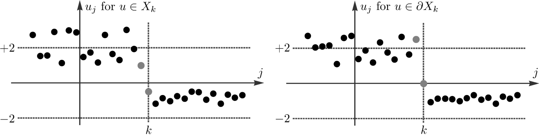
In order to make precise what we mean by single-interface solution, we define for each $k\in{\mathbb{Z}}$ the state space

\displaystyle X_{k}=\Big\{u\in\ell^{\infty}{\left({{\mathbb{Z}}}\right)}\;:\quad 0<\inf_{j<k}u_{j}\leq\sup_{j<k}u_{j}<\infty,\quad-2<\inf_{j\geq k}u_{j}\leq\sup_{j\geq k}u_{j}<0\Big\},

see Figure 3.1 for an illustration. As shown below, the dynamics for initial data chosen from $X_{k}$ is as follows: The system stays inside $X_{k}$ until some maximal time $t^{*}_{k}>0$ with $\lim_{t\to t^{*}_{k}}u_{k}{\left({t}\right)}=0$ at which $u_{k}$ undergoes a phase transition by crossing the spinodal value $0$ from below. For times $t>t^{*}_{k}$ , the system evolves inside of $X_{k+1}$ until $u_{k+1}$ changes from negative to positive phase at time $t^{*}_{k+1}>t^{*}_{k}$ . By iteration we therefore find a phase interface that moves to the right, where we allow for $t^{*}_{k}=\infty$ to account for standing interfaces.

Definition 3.1 (single-interface solution).

A continuous function $u\colon[0,\infty)\to\ell^{\infty}{\left({{\mathbb{Z}}}\right)}$ is called single-interface solution to (1.1) with potential (3.1) if there exists $k_{1}\in{\mathbb{Z}}$ along with a sequence ${\left({t^{*}_{k}}\right)}_{k\geq k_{1}}\subset(0,\infty]$ such that the following conditions are satisfied with $t^{*}_{k_{1}-1}:=0$ :

1.

For all $k\geq k_{1}$ , we have either $t^{*}_{k-1}=\infty$ or $t^{*}_{k-1}<t^{*}_{k}$ ,
2.

The function $u$ solves $\dot{u}_{j}=\laplace\Phi^{\prime}{\left({u_{j}}\right)}$ for all times $t\in[0,\infty)\setminus\{t^{*}_{k}:k\geq k_{1}\}$ ,
3.

We have $u_{k}{\left({t^{*}_{k}}\right)}=0$ and $\lim_{t\searrow t^{*}_{k}}\dot{u}_{k}{\left({t}\right)}>0$ for all $k\geq k_{1}$ with $t^{*}_{k}<\infty$ ,
4.

The function $u$ takes values in $X_{k}$ on each time interval $(t^{*}_{k-1},t^{*}_{k})$ with $t^{*}_{k-1}<\infty$ .

Moreover, a single-interface solution with $t^{*}_{k}=\infty$ for all $k\geq k_{1}$ is called a standing-interface solution.

For single-interface solutions in the sense of Definition 3.1, any $u_{k}$ is continuous at the phase transition time $t^{*}_{k}$ , whereas $p_{k}$ jumps at $t^{*}_{k}$ from $+1$ to $-1$ . Notice that it is the other way around in the macroscopic limit: when ${\varepsilon}$ tends to $0$ , $p$ becomes continuous with respect to both $\tau$ and $\xi$ , whereas $u$ jumps from $0$ to $+2$ at the phase interface, see Figure 2.9 for an illustration.

As first main result we prove that single-interface solutions exist.

Theorem 3.2 (existence and uniqueness of single-interface solutions).

For given initial data in $X_{k_{1}}$ , there exists a unique single-interface solution to (1.1) with (3.1). Moreover, this solution satisfies

\sup_{t\in[0,\infty)}\sup_{j\in\mathbb{Z}}u_{j}(t)\leq D:=\max\big\{2,\,\sup_{j\in\mathbb{Z}}u_{j}{\left({0}\right)}\big\},

and we have

\displaystyle u_{k-1}{\left({t^{*}_{k}}\right)}>2,\qquad t^{*}_{k+1}-t^{*}_{k}\geq\ln\sqrt{\frac{D+2}{D-2}},\qquad\dot{u}_{k}{\left({t^{*}_{k}}\right)}=\lim\limits_{t\searrow t^{*}_{k}}\dot{u}_{k}{\left({t}\right)}=4+\lim\limits_{t\nearrow t^{*}_{k}}\dot{u}_{k}{\left({t}\right)}\geq 4

for all $k\geq k_{1}$ with $t^{*}_{k}<\infty$ .

Proof.

We assume, without loss of generality, that $k_{1}=1$ and derive all claims by induction with respect to $k\geq k_{1}$ .

Dynamics inside of $X_{1}$ : For states $u\in X_{1}$ we have $\sgn{u_{j}}=-\sgn{\left({j-1}\right)}$ and hence

\displaystyle\dot{u}_{j}=\laplace\Phi^{\prime}{\left({u_{j}}\right)}=\laplace u_{j}+2\delta_{j}^{0}-2\delta_{j}^{1},

(3.4)

where $\delta_{j}^{k}$ is the Kronecker delta. In particular, the right hand side of (3.4) is Lipschitz continuous with respect to the $\ell^{\infty}$ -norm of $u$ and this implies the local existence of a unique solution that is smooth in time and takes values in the open set $X_{1}$ . From the definition of $X_{1}$ we also infer that

\displaystyle\begin{array}[]{rccclcl}0&\leq&\dot{u}_{j}{\left({t}\right)}+2u_{j}{\left({t}\right)}&\leq&2D&&\text{for }j<1,\\ 0&\leq&\dot{u}_{j}{\left({t}\right)}+2u_{j}{\left({t}\right)}&\leq&D+2&&\text{for }j=0,\\ -4&\leq&\dot{u}_{j}{\left({t}\right)}+2u_{j}{\left({t}\right)}&&&&\text{for }j=1,\\ -4&\leq&\dot{u}_{j}{\left({t}\right)}+2u_{j}{\left({t}\right)}&\leq&0&&\text{for }j>1,\end{array}

and the comparison principle for scalar ODEs gives

\displaystyle\begin{array}[]{rccclcl}e^{-2t}u_{j}{\left({0}\right)}&\leq&u_{j}(t)&\leq&e^{-2t}u_{j}{\left({0}\right)}+{\left({1-e^{-2t}}\right)}D&&\text{for }j<1,\\ e^{-2t}u_{j}{\left({0}\right)}-2{\left({1-e^{-2t}}\right)}&\leq&u_{j}(t)&&&&\text{for }j\geq 1,\\ &&u_{j}(t)&\leq&e^{-2t}u_{j}{\left({0}\right)}&&\text{for }j>1.\end{array}

Using these estimates, we now conclude that the local solution with values in $X_{1}$ either exists for all times (in which case we set $t^{*}_{1}:=\infty$ ) or reaches the boundary of $X_{1}$ at some time $0<t^{*}_{1}<\infty$ via $u_{1}{\left({t^{*}_{1}}\right)}=0$ . Moreover, since both $u_{1}$ and $\dot{u}_{1}$ are continuous at any $t\in[0,t^{*}_{1})$ we have $\lim_{t\nearrow t^{*}_{1}}\dot{u}_{1}{\left({t}\right)}\geq 0$ .

Phase transition at $t^{*}_{1}$ : Now suppose that $t^{*}_{1}<\infty$ . From (3.4) and the above estimate for $u_{j}{\left({t}\right)}$ we conclude that $u_{j}{\left({t}\right)}$ converges for any $j\in{\mathbb{Z}}$ as $t\nearrow t^{*}_{1}$ to some well-defined limit $u_{j}{\left({t^{*}_{1}}\right)}$ , where $u_{1}{\left({t_{1}^{*}}\right)}=0$ as well as

\displaystyle 0<\inf\limits_{j<1}u_{j}{\left({t^{*}_{1}}\right)}\leq\sup\limits_{j<1}u_{j}{\left({t^{*}_{1}}\right)}<D,\qquad-2<\inf\limits_{j>1}u_{j}{\left({t^{*}_{1}}\right)}\leq\sup\limits_{j>1}u_{j}{\left({t^{*}_{1}}\right)}<0.

We therefore have

\displaystyle\sup\limits_{j\in{\mathbb{Z}}}\left|{\laplace\Phi^{\prime}{\big(u_{j}{\left({t^{*}_{1}}\right)}\big)}}\right|\leq{C}

for some constant $C$ . On the other hand, $u_{0}{\left({t^{*}_{1}}\right)}>0$ and $-2<u_{2}{\left({t^{*}_{1}}\right)}<0$ ensure that

\displaystyle\laplace\Phi^{\prime}{\big(u_{1}{\left({t^{*}_{1}}\right)}\big)}={\Big(u_{0}{\left({t^{*}_{1}}\right)}+u_{2}{\left({t^{*}_{1}}\right)}\Big)}-{\Big(\sgn u_{0}{\left({t^{*}_{1}}\right)}+\sgn u_{2}{\left({t^{*}_{1}}\right)}-2\sgn 0\Big)}>0

thanks to $\sgn 0=+1$ . These results reveal that the vector field of the dynamical system $\dot{u}=\laplace\Phi^{\prime}{\left({u}\right)}$ is well defined in the state $u{\left({t^{*}_{1}}\right)}\in\partial X_{1}\cap\partial X_{2}$ and points into $X_{2}$ , where $\partial X_{k}$ denotes the topological boundary of $X_{k}$ in $\ell^{\infty}{\left({{\mathbb{Z}}}\right)}$ . We therefore find a time $t_{*}>t^{*}_{1}$ such that the local solution to the microscopic dynamics from the first step has unique continuation to the time interval $[0,t_{*})$ with $u{\left({t}\right)}\in{X_{2}}$ for all $t\in(t^{*}_{1},t_{*})$ . By construction, $u_{j}$ and $\dot{u}_{j}$ are continuous at $t^{*}_{1}$ for $j\neq 1$ , whereas

\displaystyle{u}_{1}{\left({t^{*}_{1}}\right)}=\lim_{t\to t^{*}_{1}}{u}_{1}{\left({t}\right)}=0,\qquad\dot{u}_{1}{\left({t^{*}_{1}}\right)}=\lim_{t\searrow t^{*}_{1}}\dot{u}_{1}{\left({t}\right)}=4+\lim_{t\nearrow t^{*}_{1}}\dot{u}_{1}{\left({t}\right)}\geq 4.

thanks to $\sgn u_{1}{\left({t^{*}_{1}}\right)}=\lim_{t\searrow t^{*}_{1}}\sgn u_{1}{\left({t}\right)}=+1$ and $\lim_{t\nearrow t^{*}_{1}}u_{1}{\left({t^{*}_{1}}\right)}=-1$ . Finally, repeating all arguments from the first step we show that this solution in $X_{2}$ exists uniquely until a time $t^{*}_{2}$ with $t^{*}_{1}<t^{*}_{2}\leq\infty$ and $u_{2}{\left({t^{*}_{2}}\right)}=0$ in case of $t^{*}_{2}<\infty$ .

Condition for $u_{0}{\left({t^{*}_{1}}\right)}$ and lower bound for $t^{*}_{2}-t^{*}_{1}$ : For $0<t<t^{*}_{1}$ we infer from (3.4) that

\displaystyle\dot{u}_{1}{\left({t}\right)}

\displaystyle={\big(u_{0}{\left({t}\right)}+u_{2}{\left({t}\right)}-2u_{1}(t)\big)}-{\big({\left({+1}\right)}+{\left({-1}\right)}-2{\left({-1}\right)}\big)}\leq u_{0}{\left({t}\right)}+u_{2}{\left({t}\right)}-2u_{1}{\left({t}\right)}-2.

Passing to the limit $t\nearrow t^{*}_{1}$ we therefore get

\displaystyle 0\leq\dot{u}_{1}{\left({t^{*}_{1}}\right)}\leq u_{0}{\left({t^{*}_{1}}\right)}+u_{2}{\left({t^{*}_{1}}\right)}-2<u_{0}{\left({t^{*}_{1}}\right)}-2

and hence $u_{0}{\left({t^{*}_{1}}\right)}>2$ . In the same way we prove $u_{1}{\left({t^{*}_{2}}\right)}>2$ and conclude that the interface can shift from $k=1$ to $k=2$ at time $t^{*}_{2}$ only if

\displaystyle 2<u_{1}{\left({t^{*}_{2}}\right)}.

Moreover, $u{\left({t}\right)}\in X_{2}$ for all $t\in(t^{*}_{1},t^{*}_{2})$ implies

\displaystyle\dot{u}_{1}{\left({t}\right)}

\displaystyle={\big(u_{0}{\left({t}\right)}+u_{2}{\left({t}\right)}-2u_{1}(t)\big)}-{\big({\left({+1}\right)}+{\left({-1}\right)}-2{\left({+1}\right)}\big)}\leq D+2-2u_{1}{\left({t}\right)}.

By the comparison principle we therefore have

\displaystyle u_{1}{\left({t}\right)}\leq{\left({1-e^{-2t+2t^{*}_{1}}}\right)}\frac{D+2}{2},

and setting $t=t^{*}_{2}$ we obtain the estimate for $t^{*}_{2}-t^{*}_{1}$ .

Final step: All arguments derived above can easily be iterated, so the assertions of Theorem 3.2 are proved by induction. In particular, the lower bound for $t^{*}_{k+1}-t^{*}_{k}$ ensures that the solution exists for all times $t\geq 0$ . ∎

Remark 3.3.

Theorem 3.2 can be adapted to finite lattice systems with $j=1,\ldots,M$ provided that the corresponding ODE system is closed by imposing

1.

either homogeneous Neumann boundary conditions via $u_{0}{\left({t}\right)}=u_{1}{\left({t}\right)}$ and $u_{M+1}{\left({t}\right)}=u_{M}{\left({t}\right)}$ ,
2.

or inhomogeneous Dirichlet boundary conditions via $u_{0}{\left({t}\right)}\equiv c_{1}>0$ and $u_{M+1}{\left({t}\right)}\equiv c_{2}<0$ ,

where $j=0$ and $j=M+1$ are the ghost indices.

The proof of Theorem 3.2 reveals that the condition $\sgn 0=1$ (or equivalently, the right-sided continuity of $\Phi^{\prime}$ ) is crucial for the microscopic dynamics to be well defined after the phase transition time $t^{*}_{k}$ as it guarantees that $u_{k}{\left({t^{*}_{k}}\right)}=0$ implies the strict inequality $\dot{u}_{k}{\left({t^{*}_{k}+0}\right)}>0$ . Our convention (3) is therefore implicitly but intimately related to phase interfaces that propagate into the phase $u<0$ (to observe phase propagation into to the other phase $u>0$ , one has to set $\sgn{0}=-1$ ). This subtle direction selection reflects that the spinodal region is actually an isolated point and can be regarded as the degenerate analogue to the hysteresis flow rule (1.10).

Corollary 3.4 (criterion for standing interfaces).

For single-interface initial data

u{\left({0}\right)}\in X_{k_{1}}\quad\text{ with }\quad\sup_{j\in{\mathbb{Z}}}u_{j}{\left({0}\right)}\leq 2

we find $t^{*}_{k_{1}}=\infty$ and hence a standing-interface solution.

We finally characterize the evolution of $p_{j}{\left({t}\right)}=\Phi^{\prime}(u_{j}(t))$ for single-interface solutions. The key observations are as follows:

1.

$p$ solves the linear discrete heat equation $\dot{p}=\laplace{p}$ on each time interval $(t^{*}_{k},t^{*}_{k+1})$ because $u{\left({t}\right)}\in X_{k}$ implies $p_{j}{\left({t}\right)}=u_{j}{\left({t}\right)}+\sgn{\left({j-k}\right)}$ and hence $\dot{p}_{j}{\left({t}\right)}=\dot{u}_{j}{\left({t}\right)}$ .
2.

At each phase transition time $t^{*}_{k}<\infty$ , the value of $p_{k}$ jumps down according to

$\displaystyle\lim\limits_{t\nearrow t^{*}_{k}}p_{k}{\left({t}\right)}=+1,\qquad\lim\limits_{t\searrow t^{*}_{k}}p_{k}{\left({t}\right)}=-1$

but we have $\lim_{t\nearrow t^{*}_{k}}p_{j}{\left({t}\right)}=\lim_{t\searrow t^{*}_{k}}p_{j}{\left({t}\right)}$ for all $j\neq{k}$ .

The dynamics of $p$ can therefore be interpreted as solving the linear discrete heat equation for $t\geq 0$ where at each phase transition time $t^{*}_{k}$ we perturb the system by adding $-2\delta_{j}^{k}$ to the current state. Combining this interpretation with the superposition principle we conclude that $p$ consists of a regular part $q$ and a singular part $r$ , which account for effects of the initial data and the perturbations induced by the phase transitions, respectively. In particular, denoting by $g$ the discrete heat kernel, that is

	$\displaystyle\dot{g}_{j}(t)$	$\displaystyle=\laplace g_{j}(t),$		(3.5)
	$\displaystyle g_{j}(0)$	$\displaystyle=\delta_{j}^{0},$		(3.5)

we arrive at the following result, see also Figure 3.2.

Corollary 3.5 (decomposition of $p$ ).

For each single-interface solution we have

p_{j}(t)=q_{j}(t)+r_{j}{\left({t}\right)},

with

\displaystyle r_{j}{\left({t}\right)}:=-2\sum_{k\geq k_{1}}\chi_{\left\{t\geq t^{*}_{k}\right\}}(t)g_{j-k}(t-t^{*}_{k}),

where $q$ is the solution of the discrete heat equation with initial data $q_{j}{\left({0}\right)}=p_{j}{\left({0}\right)}$ and $\chi_{J}$ denotes the indicator function of the set $J$ .

The decomposition formula from Corollary 3.5 is crucial for our analysis. In particular, the decay and continuity properties of the discrete heat kernel, see appendix A, enable us to estimate the impact of the sequence of singularities induced by the phase transitions. Notice however, that the evolution of $p$ is still nonlinear as the phase transition times $t^{*}_{k}$ depend on $p$ itself.

3.2 Upper bounds for the macroscopic interface speed

In Theorem 3.2 we have shown that single-interface solutions exist. In order to pass to the macroscopic limit, we must however guarantee that the corresponding macroscopic interface speed is at most of order ${O{\left({1}\right)}}$ . More precisely, for a given macroscopic distance $\delta>0$ we have to ensure that the macroscopic time ${\varepsilon}^{2}t^{*}_{\lfloor\delta/{\varepsilon}\rfloor}$ is bounded from below by some constant independent of ${\varepsilon}$ , where $\lfloor{x}\rfloor$ is shorthand for the integer part of $x$ . The derivation of this lower bound is actually at the heart of our convergence proof and requires a careful quantitative analysis of the lattice dynamics. In this paper we restrict ourselves to the most simple case and suppose that the initial data are compatible with the macroscopic limit model. We also assume without loss of generality that the macroscopic interface is initially located at $\xi=0$ .

Assumption 3.6 (macroscopic single-interface initial data).

The initial data $u{\left({0}\right)}$ belong to $X_{1}$ and $p{\left({0}\right)}=\Phi^{\prime}{\left({u{\left({0}\right)}}\right)}$ satisfies

\displaystyle\left|{\laplace p_{0}{\left({0}\right)}}\right|\leq\beta{\varepsilon},\qquad\sup\limits_{j\in{\mathbb{Z}}}\left|{\nabla_{+}p_{j}{\left({0}\right)}}\right|\leq\alpha{\varepsilon},\qquad\sup\limits_{j\neq 0}\left|{\laplace p_{j}{\left({0}\right)}}\right|\leq\alpha{\varepsilon}^{2}.

for two constants $\alpha$ and $\beta$ independent of ${\varepsilon}$ .

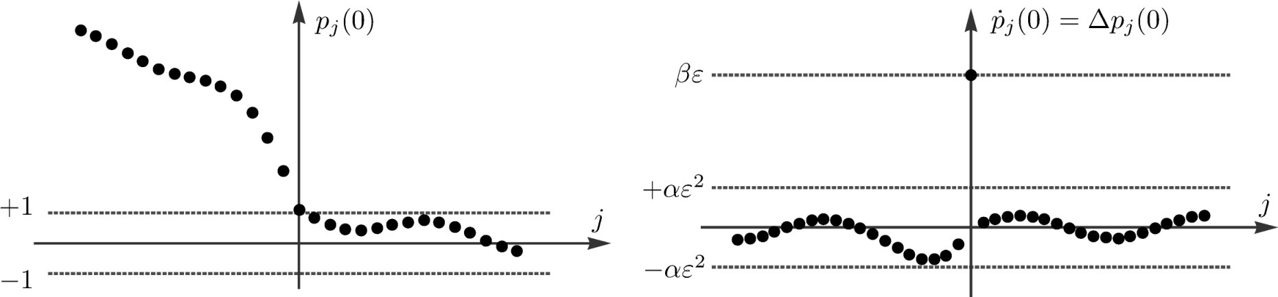
Assumption 3.6 is motivated by the limit dynamics, see also Figure 3.3 for an illustration. In fact, the prototypical example for macroscopic single-interface data is

\displaystyle p_{j}{\left({t}\right)}=P_{\rm ini}{\left({{\varepsilon}j}\right)}+c_{\varepsilon},\qquad u_{j}{\left({0}\right)}=p_{j}{\left({t}\right)}+\sgn{\left({-j}\right)}

(3.6)

where $c_{\varepsilon}$ is a constant and $P_{\rm ini}$ some given macroscopic function independent of ${\varepsilon}$ such that:

$P_{\rm ini}$ is bounded and continuous for all $\xi\in{\mathbb{R}}$ with

\displaystyle P_{\rm ini}{\left({\xi}\right)}>1\quad\text{for}\quad\xi<0\qquad\text{and}\quad-1<P_{\rm ini}{\left({\xi}\right)}<1\quad\text{for}\quad\xi>0

and

\displaystyle\liminf_{\xi\to-\infty}P_{\rm ini}{\left({\xi}\right)}>1\qquad\text{and}\qquad-1<\liminf_{\xi\to+\infty}P_{\rm ini}{\left({\xi}\right)}\leq\limsup_{\xi\to+\infty}P_{\rm ini}{\left({\xi}\right)}<+1.

$P_{\rm ini}$ is twice continuously differentiable for $\xi<0$ and $\xi>0$ with

\displaystyle\beta:=\lim\limits_{\xi\searrow 0}\left|{P_{\rm ini}^{\prime}{\left({+\xi}\right)}-P_{\rm ini}^{\prime}{\left({-\xi}\right)}}\right|<\infty,\qquad\alpha:=\sup\limits_{\xi\neq 0}\left|{P_{\rm ini}^{\prime}{\left({\xi}\right)}}\right|+\left|{P_{\rm ini}^{\prime\prime}{\left({\xi}\right)}}\right|<\infty,

3.

$c_{\varepsilon}>0$ is sufficiently small with $c_{\varepsilon}\to 0$ as ${\varepsilon}\to 0$ and chosen such that $t^{*}_{1}>0$ , that means $u_{j}{\left({0}\right)}>0$ for all $j\leq 0$ and $u_{j}{\left({0}\right)}<0$ for all $j\geq 1$ .

Corollary 3.7 (bounds for the regular part $q$ ).

We have

\displaystyle\left|{\nabla_{+}q_{j}{\left({t}\right)}}\right|\leq{\alpha}{\varepsilon}\qquad\text{and}\qquad|{\dot{q}_{j}{\left({t}\right)}}|=\left|{\laplace q_{j}{\left({t}\right)}}\right|\leq{\alpha}{\varepsilon}^{2}+\beta{\varepsilon}g_{0}{\left({t}\right)}

for all $t\geq 0$ , $j\in{\mathbb{Z}}$ , and ${\varepsilon}>0$ .

Proof.

By construction and Assumption 3.6 we have

\displaystyle\tfrac{\,\mathrm{d}}{\,\mathrm{d}t}\dot{q}_{j}{\left({t}\right)}=\laplace\dot{q}_{j}{\left({t}\right)},\qquad|{\dot{q}_{j}{\left({0}\right)}}|=\left|{\dot{p}_{j}{\left({0}\right)}}\right|=\left|{\dot{u}_{j}{\left({0}\right)}}\right|=\left|{\laplace{p}_{j}{\left({0}\right)}}\right|\leq\alpha{\varepsilon}^{2}+\beta{\varepsilon}\delta_{j}^{0}

as well as

\displaystyle\tfrac{\,\mathrm{d}}{\,\mathrm{d}t}\nabla_{+}{q}_{j}{\left({t}\right)}=\laplace\nabla_{+}{q}_{j}{\left({t}\right)},\qquad\left|{\nabla_{+}{q}_{j}{\left({0}\right)}}\right|=\left|{\nabla_{+}{p}_{j}{\left({0}\right)}}\right|\leq\alpha{\varepsilon}.

The claim now follows using both the superposition and the maximum principle for the discrete heat equation. ∎

We remark that the assertions of Corollary 3.7 are sufficient for showing that the macroscopic interface speed is bounded. All results derived below therefore hold (with different constants) even in the case that

1.

$\left|{\nabla_{+}{p}_{j}{\left({0}\right)}}\right|\leq\alpha{\varepsilon}$ and $\left|{\laplace p_{j}{\left({0}\right)}}\right|\leq\beta{\varepsilon}$ for all $j\in{\mathbb{Z}}$ ,
2.

$\left|{\laplace p_{j}{\left({0}\right)}}\right|\leq\alpha{\varepsilon}^{2}$ for almost all $j\in{\mathbb{Z}}$ ,

that means the derivative of the function $P_{\rm ini}$ from (3.6) can even be discontinuous at finitely many points.

We are now able to derive upper bounds for the macroscopic interface speed. To this end we prove that Assumption 3.6 implies that the time $t^{*}_{k+1}-t^{*}_{k}$ between two adjacent phase transitions is mesoscopic as it can be bounded from below by $1/{\varepsilon}$ (recall that Theorem 3.2 provides only $t^{*}_{k+1}-t^{*}_{k}\geq 2/{\left({D-2}\right)}$ ). Our considerations are based on the estimate

\displaystyle 2\leq p_{k}{\left({t^{*}_{k+1}}\right)}-p_{k}{\left({t^{*}_{k}}\right)}=\int_{t^{*}_{k}}^{t^{*}_{k+1}}\dot{p}_{k}(t)\,\mathrm{d}t=\int_{t^{*}_{k}}^{t^{*}_{k+1}}\dot{q}_{k}(t)\,\mathrm{d}t-2\sum_{n=1}^{k}\int_{t^{*}_{k}}^{t^{*}_{k+1}}\dot{g}_{k-n}(t-t^{*}_{n})\,\mathrm{d}t,

(3.7)

which follows from combining the conditions $u_{k}{\left({t^{*}_{k}}\right)}=0$ and $u_{k}(t^{*}_{k+1})\geq 2$ with the representation formula from Corollary 3.5.

Lemma 3.8 (refined lower bound for the time between two phase transitions).

For any $\tau_{\rm fin}>0$ there is a constant $d_{*}>0$ , which depends on $\alpha$ , $\beta$ , and $\tau_{\rm fin}$ , along with a constant $0<{\varepsilon}_{*}<1$ , which depends only on $\alpha$ and $\beta$ , such that

{\varepsilon}{\left({t^{*}_{k+1}-t^{*}_{k}}\right)}\geq 2d_{*}

holds for all $k\geq 1$ with $0\leq t^{*}_{k}\leq\tau_{\rm fin}/{\varepsilon}^{2}$ provided that ${\varepsilon}\leq{\varepsilon}_{*}$ .

Proof.

In what follows we consider $k\geq 1$ with $t^{*}_{k}<\tau_{\rm fin}/{\varepsilon}^{2}$ and denote by $c$ and $C$ generic constants independent of ${\alpha}$ , $\beta$ , and ${\varepsilon}$ .

Weaker variant of (3.7): In order to study the implications of (3.7), we first simplify the right hand side as follows. By Lemma A.2 we have

\displaystyle-\sum_{n=1}^{k}\int_{t^{*}_{k}}^{t^{*}_{k+1}}\dot{g}_{k-n}(t-t^{*}_{n})\,\mathrm{d}t

\displaystyle\leq-\sum_{n=1}^{k}\int_{t^{*}_{k}}^{t^{*}_{k+1}}\dot{g}_{0}(t-t^{*}_{n})\,\mathrm{d}t=\sum_{n=1}^{k}g_{0}{\left({t^{*}_{k}-t^{*}_{n}}\right)}-\sum_{n=1}^{k}g_{0}{\left({t^{*}_{k+1}-t^{*}_{n}}\right)}.

whereas Corollary 3.7 provides

\displaystyle\int_{t^{*}_{k}}^{t^{*}_{k+1}}\dot{q}_{k}(t)\,\mathrm{d}t\leq\int_{t^{*}_{k}}^{t^{*}_{k+1}}{\big(\alpha{\varepsilon}^{2}+\beta{\varepsilon}g_{0}{\left({t}\right)}\big)}\,\mathrm{d}t

Rearranging terms and using $g_{0}(0)=1$ , inequality (3.7) becomes

\sum_{n=1}^{k}g_{0}(t^{*}_{k+1}-t^{*}_{n})\leq\frac{1}{2}\int_{t^{*}_{k}}^{t^{*}_{k+1}}{\left({\alpha{\varepsilon}^{2}+\beta{\varepsilon}g_{0}(t)}\right)}\,\mathrm{d}t+\sum_{n=1}^{k-1}g_{0}(t^{*}_{k}-t^{*}_{n}),

and writing $s_{k}:=t^{*}_{k+1}-t^{*}_{k}$ we arrive at

\sum_{n=1}^{k}g_{0}(s_{k}+\cdots+s_{n})\leq\frac{1}{2}\int_{t^{*}_{k}}^{t^{*}_{k}+s_{k}}{\left({\alpha{\varepsilon}^{2}+\beta{\varepsilon}g_{0}(t)}\right)}\,\mathrm{d}t+\sum_{n=1}^{k-1}g_{0}(s_{k-1}+\cdots+s_{n}).

(3.8)

In the remainder of this proof we transform this inequality into a lower bound for $s_{k}$ .

Estimate for $k=1$ : Inequality (3.8) combined with Lemma A.1 provides

g_{0}(s_{1})\leq\tfrac{1}{2}\int_{t^{*}_{1}}^{t^{*}_{1}+s_{1}}{\left({\alpha{\varepsilon}^{2}+\beta{\varepsilon}g_{0}(t)}\right)}\,\mathrm{d}t\leq\tfrac{1}{2}\int_{0}^{s_{1}}{\left({\alpha{\varepsilon}^{2}+\beta{\varepsilon}g_{0}(t)}\right)}\,\mathrm{d}t,

and we deduce that there exists ${\varepsilon}_{*}>0$ , which depends on $\alpha$ and $\beta$ , such that $s_{1}\geq 1$ for all ${\varepsilon}\leq{\varepsilon}_{*}$ . We employ Lemma A.2 again to estimate

\frac{c}{\sqrt{s_{1}}}\leq{C}{\big(\alpha{\varepsilon}^{2}+\beta{\varepsilon}\sqrt{s_{1}}\big)},

and this gives

{\varepsilon}s_{1}\geq d_{1}>0

for some constant $d_{1}$ which depends on $\alpha$ and $\beta$ but not on ${\varepsilon}$ . For $\beta=0$ we even find ${\varepsilon}^{4/3}s_{1}\geq d_{1}$ .

Estimate for $k>1$ in a special case: For the following considerations we further suppose that

\displaystyle s_{k}<\min\limits_{n=1,\ldots,k-1}s_{n}.

Since $g_{0}$ is strictly decreasing, we therefore get

g_{0}(s_{k}+\cdots+s_{n+1})>g_{0}(s_{k-1}+\cdots+s_{n})

for all $n=1,\ldots,k-1$ , and hence

g_{0}(s_{k}+\cdots+s_{1})<\frac{1}{2}\int_{t^{*}_{k}}^{t^{*}_{k}+s_{k}}{\left({\alpha{\varepsilon}^{2}+\beta{\varepsilon}g_{0}(t)}\right)}\,\mathrm{d}t,

thanks to (3.8). This implies $f_{k}{\left({s_{k}}\right)}<0$ for

f_{k}{\left({s}\right)}:=g_{0}(s+t^{*}_{k})-\frac{1}{2}\int_{t^{*}_{k}}^{t^{*}_{k}+s}{\left({\alpha{\varepsilon}^{2}+\beta{\varepsilon}g_{0}(t)}\right)}\,\mathrm{d}t,

where we used that $g_{0}(s_{k}+\cdots+s_{1})=g_{0}(s_{k}+t^{*}_{k}-t^{*}_{1})\geq g_{0}(s_{k}+t^{*}_{k})$ . The properties of $g_{0}$ , see Lemma A.1 once more, guarantee that the function $f_{k}$ is convex, continuous, and strictly decreasing in $s$ . Therefore, and in view of $f_{k}{\left({0}\right)}>0$ and $\lim_{s\to\infty}f_{k}{\left({s}\right)}=-\infty$ , we conclude that $f_{k}$ has a unique zero $\bar{s}_{k}$ with $\bar{s}_{k}<s_{k}$ . Due to convexity of $f_{k}$ we also find

\displaystyle\hat{s}_{k}<\bar{s}_{k}<s_{k},

where $\hat{s}_{k}:=-f_{k}{\left({0}\right)}/f_{k}^{\prime}{\left({0}\right)}$ is the first approximation to $\bar{s}_{k}$ when starting the Newton algorithm at $s=0$ . By direct computations we now verify

\hat{s}_{k}=\frac{g_{0}{\left({t^{*}_{k}}\right)}}{-\dot{g}_{0}{\left({t^{*}_{k}}\right)}+\frac{\alpha{\varepsilon}^{2}}{2}+\frac{\beta{\varepsilon}}{2}g_{0}(t^{*}_{k})},

and using $t^{*}_{k}\geq s_{1}\geq 1$ as well as Lemma A.2 we obtain

\displaystyle\hat{s}_{k}\geq\frac{c{\left({t^{*}_{k}}\right)}^{-1/2}}{C{\left({t^{*}_{k}}\right)}^{-3/2}+\alpha{\varepsilon}^{2}+{C}\beta{\varepsilon}{\left({t^{*}_{k}}\right)}^{-1/2}}\geq\frac{c}{{\left({t^{*}_{k}}\right)}^{-1}+\alpha{\varepsilon}^{2}{\left({t^{*}_{k}}\right)}^{1/2}+\beta{\varepsilon}},

and hence

\displaystyle{\varepsilon}s_{k}\geq\frac{c}{d_{1}^{-1}+\alpha\tau_{\rm fin}^{1/2}+\beta}=:d_{2}

where we used that $t^{*}_{k}\geq s_{1}\geq d_{1}/{\varepsilon}$ and $t^{*}_{k}\leq\tau_{\rm fin}/{\varepsilon}^{2}$ .

Estimate for $k>1$ in the general case: We have established the estimate ${\varepsilon}s_{1}\geq d_{1}$ as well as the implication

\displaystyle{\varepsilon}s_{k}\leq\min\{{\varepsilon}s_{1},\ldots,{\varepsilon}s_{k-1}\}\quad\implies\quad{\varepsilon}s_{k}\geq d_{2},

and the desired estimate for $s_{k}$ follows with $d_{*}:=\tfrac{1}{2}\min\{d_{1},d_{2}\}$ by induction. ∎

From Lemma 3.8 we immediately obtain $t^{*}_{k}\geq 2kd_{*}/{\varepsilon}$ and we deduce for each macroscopic time $\tau_{\rm fin}$ that at most $\tau_{\rm fin}/{\left({2{\varepsilon}d_{*}}\right)}$ phase transitions can happen for $\tau\leq\tau_{\rm fin}$ , shifting the interface over a macroscopic distance smaller than $\tau_{\rm fin}/{\left({2d_{*}}\right)}$ .

We conclude this section with some comments concerning the microscopic fluctuations caused by the phase transition of $u_{k}$ at $t^{*}_{k}$ . The properties of the discrete heat kernel imply that the amplitude as well the inverse length of the effective spatial support scale with

\displaystyle\frac{{\varepsilon}}{\sqrt{{\varepsilon}^{2}+{\left({\tau-{\varepsilon}^{2}t^{*}_{k}}\right)}}},

which decays quite rapidly within a macroscopic time of order ${\varepsilon}^{2}$ but much slower afterwards. In particular, when $u_{k+1}$ undergoes the next phase transition at time $t^{*}_{k+1}$ , the fluctuations evoked by $u_{k}$ have reached an amplitude of order ${\varepsilon}^{1/2}$ and spread over a macroscopic length of order ${\varepsilon}^{-1/2}$ . Similarly, the amplitude of the velocity fluctuations at time $t^{*}_{k+1}$ is of order ${\varepsilon}^{3/2}$ .

These scaling arguments, especially the fractional powers of ${\varepsilon}$ , reveal that macroscopic single-interface data are not invariant under the dynamics. In other words, the lattice data at times $t\lessapprox t^{*}_{k}$ – this means just before the phase transitions – do not satisfy Assumption 3.6, and we conclude that interface propagation in discrete forward-backward diffusion equations is not only a two-scale but a genuine multi-scale problem.

3.3 Macroscopic continuity and compactness results

In order to pass to the macroscopic limit ${\varepsilon}\to 0$ , we regard the discrete data $p_{j}{\left({t}\right)}$ , $q_{j}{\left({t}\right)}$ , and $r_{j}{\left({t}\right)}$ as piecewise constant functions with respect to the macroscopic coordinates $(\tau,\xi)$ . More precisely, we set

\displaystyle P_{\varepsilon}{\big({\tau},\,{\xi+\zeta}\big)}:=p_{\xi/{\varepsilon}}{\left({\tau/{\varepsilon}^{2}}\right)}\qquad\text{for all}\quad\tau\geq 0,\quad\xi\in{\varepsilon}{\mathbb{Z}},\quad\zeta\in[-{\varepsilon}/2,+{\varepsilon}/2)

and define $Q_{\varepsilon}$ and $R_{\varepsilon}$ by analogous formulas. We further introduce the macroscopic interface position

\displaystyle\xi^{*}_{\varepsilon}{\left({\tau}\right)}:={\varepsilon}\sum_{k=1}^{\infty}{k}\chi_{[t^{*}_{k},t^{*}_{k+1})}{\left({\tau/{\varepsilon}^{2}}\right)}\qquad\text{for all}\quad\tau\geq 0,

as a piecewise constant function in time that jumps at the macroscopic phase transitions times defined by

\displaystyle\tau^{*}_{k,\,{\varepsilon}}:={\varepsilon}^{2}t^{*}_{k}\qquad\text{for all}\quad k\in{\mathbb{Z}}.

In what follows we fix a macroscopic final time $0<\tau_{\rm fin}<\infty$ and wish to pass to the limit ${\varepsilon}\to 0$ on the macroscopic time-space domain

\displaystyle{\Omega}:=I\times{\mathbb{R}},\qquad I:=[0,\tau_{\rm fin}].

To this end, we recall that Lemma 3.8 provides constants $d_{*}>0$ and $0<{\varepsilon}_{*}\leq 1$ such that

\displaystyle K_{\varepsilon}\leq\frac{\tau_{\rm fin}}{2d_{*}{\varepsilon}},\qquad\inf\limits_{k=1,\ldots,K_{\varepsilon}}\tau^{*}_{k+1,\,{\varepsilon}}-\tau^{*}_{k,\,{\varepsilon}}\geq 2d_{*}{\varepsilon}

(3.9)

holds for all $0<{\varepsilon}\leq{\varepsilon}_{*}$ , where

K_{\varepsilon}:=\max\Big\{k\in{\mathbb{Z}}\;:\;\tau^{*}_{k,\,{\varepsilon}}<\tau_{\rm fin}\Big\}

is the number phase transitions taking place in the microscopic time interval $[0,\tau_{\rm fin}/{\varepsilon}^{2}]$ . Notice that $d_{*}$ , ${\varepsilon}_{*}$ , and all constants derived below depend on $\tau_{\rm fin}$ and on the initial data via $\alpha$ and $\beta$ .

Our first result in this section concerns the compactness of the discrete interface curves $\xi^{*}_{\varepsilon}$ .

Lemma 3.9 (compactness of interface curves).

The family ${\left({\xi_{*}}\right)}_{0<{\varepsilon}\leq{\varepsilon}_{*}}$ is compact in ${\mathsf{L}}^{\infty}{\left({I}\right)}$ and each limit curve is Lipschitz continuous.

Proof.

We define a piecewise linear function $\bar{\xi}^{*}_{\varepsilon}$ on $[0,\tau_{\rm fin}]$ by the condition

\displaystyle\bar{\xi}^{*}_{\varepsilon}{\left({\tau^{*}_{k,\,{\varepsilon}}}\right)}=\xi^{*}_{\varepsilon}{\left({\tau^{*}_{k,\,{\varepsilon}}}\right)}

for all $k=1,\ldots,K_{\varepsilon}$ and $\bar{\xi}^{*}_{\varepsilon}{\left({\tau_{\rm fin}}\right)}=\xi^{*}_{\varepsilon}(\tau^{*}_{K_{\varepsilon},\,{\varepsilon}})$ . We readily check that

\displaystyle\big|{\bar{\xi}^{*}_{\varepsilon}{\left({\tau}\right)}-\xi^{*}_{\varepsilon}{\left({\tau}\right)}}\big|\leq{\varepsilon},\qquad 0\leq{\textstyle\frac{\mathrm{d}}{\mathrm{d}{\tau}}}\bar{\xi}^{*}_{\varepsilon}{\left({\tau}\right)}\leq\frac{{\varepsilon}}{2d_{*}{\varepsilon}}

for almost all $\tau\in[0,\tau_{\rm fin}]$ , and conclude that the family ${\left({\bar{\xi}^{*}_{\varepsilon}}\right)}_{0<{\varepsilon}\leq{\varepsilon}_{*}}$ is bounded in ${\mathsf{C}}^{0,1}(I)$ . All claims hence follow from standard results in real analysis. ∎

Our main goal this section is to derive compactness result for $R_{\varepsilon}$ and $Q_{\varepsilon}$ that imply ${\left({i}\right)}$ the existence of pointwise convergent subsequences, and ${\left({ii}\right)}$ the continuity of any limit function. In a preparatory step we next derive an auxiliary result for piecewise constant functions $F_{\varepsilon}$ on ${\Omega}$ revealing that for ${\mathsf{L}}^{\infty}$ -compactness it is sufficient to establish uniform Hölder estimates with respect to $\tau\in{I}$ and discrete $\xi\in{\varepsilon}{\mathbb{Z}}$ . Here piecewise constant means, as above, continuous with respect to $\tau$ but spatially constant in each interval $\xi\in[{\varepsilon}j-{\varepsilon}/2,\,{\varepsilon}j+{\varepsilon}/2)$ , $j\in{\mathbb{Z}}$ . Our auxiliary result and its proof are straight forward and can very likely be found somewhere in the literature on numerical analysis (though we are not aware of any reference).

Lemma 3.10 (compactness criterion for piecewise constant functions).

Let ${\left({F_{\varepsilon}}\right)}_{0<{\varepsilon}\leq{\varepsilon}_{*}}$ be a family of bounded and piecewise constant functions on ${\Omega}$ , and suppose that there exist constants ${\gamma}_{1},{\gamma}_{2}\in(0,1]$ and $C>0$ such that

\displaystyle\big|{F_{\varepsilon}{\left({\tau_{2}},\,{\xi_{2}}\right)}-F_{\varepsilon}{\left({\tau_{1}},\,{\xi_{1}}\right)}}\big|\leq{C}{\big(\big|{\tau_{2}-\tau_{1}}\big|^{{\gamma}_{1}}+\big|{\xi_{2}-\xi_{1}}\big|^{{\gamma}_{2}}\big)}

holds for all $0<{\varepsilon}\leq{\varepsilon}_{*}$ , every $\tau_{1},\tau_{2}\in{I}$ , and all $\xi_{1},\xi_{2}\in{\varepsilon}{\mathbb{Z}}$ . Then this family is compact in ${\mathsf{L}}^{\infty}{\left({{\Omega}}\right)}$ and any limit function is locally Hölder continuous with exponent $\min\{{\gamma}_{1},{\gamma}_{2}\}$ .

Proof.

For each ${\varepsilon}$ we define a piecewise linear function $\bar{F}_{\varepsilon}$ by

\displaystyle\bar{F}_{\varepsilon}{\left({\tau},\,{\bar{\xi}}\right)}=F_{\varepsilon}{\left({\tau},\,{\bar{\xi}}\right)}\qquad\text{for all}\quad\tau\in{I},\quad\bar{\xi}\in{\varepsilon}{\mathbb{Z}},

and our assumptions yield the Hölder continuity of $\bar{F}_{\varepsilon}$ with respect to time, that means

\displaystyle\big|{\bar{F}_{\varepsilon}{\left({\tau_{2}},\,{\xi}\right)}-\bar{F}_{\varepsilon}{\left({\tau_{1}},\,{\xi}\right)}}\big|\leq C\left|{\tau_{2}-\tau_{1}}\right|^{{\gamma}_{1}}

for all $\xi\in{\mathbb{R}}$ and $\tau_{1},\tau_{2}\in{I}$ . Moreover, since $\bar{F}_{\varepsilon}$ is piecewise linear with respect to $\xi$ and due to

\displaystyle\big|{F_{\varepsilon}{\left({\tau},\,{\bar{\xi}}\right)}}\big|\leq{C},\qquad\left|{\frac{F_{\varepsilon}{\left({\tau},\,{\bar{\xi}\pm{\varepsilon}}\right)}-F_{\varepsilon}{\left({\tau},\,{\bar{\xi}}\right)}}{{\varepsilon}}}\right|\leq{C}{\varepsilon}^{{\gamma}_{2}-1}

we verify – discussing the cases $\sgn{\zeta_{1}}=\sgn{\zeta_{2}}$ and $\sgn{\zeta_{1}}\neq\sgn{\zeta_{2}}$ separately – the estimate

\displaystyle\big|{\bar{F}_{\varepsilon}{\left({\tau},\,{\bar{\xi}+\zeta_{2}}\right)}-\bar{F}_{\varepsilon}{\left({\tau},\,{\bar{\xi}+\zeta_{1}}\right)}}\big|\leq C{\varepsilon}^{{\gamma}_{2}-1}\left|{\zeta_{2}-\zeta_{1}}\right|\leq C\left|{\zeta_{2}-\zeta_{1}}\right|^{{\gamma}_{2}}

(3.10)

for all $\tau\in{I}$ , $\bar{\xi}\in{\varepsilon}{\mathbb{Z}}$ , and all $\zeta_{1},\zeta_{2}\in[-{\varepsilon},+{\varepsilon}]$ . In particular, setting $\zeta_{1}=0$ and taking the supremum over $\bar{\xi}$ and $\zeta_{2}$ we obtain the convergence estimate

\displaystyle\|{F_{\varepsilon}-\bar{F}_{\varepsilon}}\|_{{\mathsf{L}}^{\infty}{\left({{\Omega}}\right)}}\leq C{\varepsilon}^{{\gamma}_{2}}.

We next show that $\bar{F}_{\varepsilon}$ is Hölder continuous with respect to $\xi$ . To this end, let $\tau\in{I}$ and $\xi_{1},\xi_{2}\in{\mathbb{R}}$ be given and denote by $\bar{\xi}_{i}$ the natural projection of $\xi_{i}$ to ${\varepsilon}{\mathbb{Z}}$ , that means $\left|{\bar{\xi}_{i}-\xi_{i}}\right|\leq{\varepsilon}/2$ . For $\left|{\xi_{1}-\xi_{2}}\right|\leq{\varepsilon}/2$ we have $\xi_{1},\xi_{2}\in[\bar{\xi}_{1}-{\varepsilon},\bar{\xi}_{1}+{\varepsilon}]$ and are hence done by (3.10). In the case of $\left|{\xi_{2}-\xi_{1}}\right|>{\varepsilon}/2$ we combine our assumptions of $F_{\varepsilon}$ with (3.10) and the triangle inequality to obtain

	$\displaystyle\big\|{\bar{F}_{\varepsilon}{\left({\tau},\,{\xi_{2}}\right)}-\bar{F}_{\varepsilon}{\left({\tau},\,{\xi_{1}}\right)}}\big\|$	$\displaystyle\leq C\left\|{\bar{\xi}_{2}-\bar{\xi}_{1}}\right\|^{{\gamma}_{2}}+C{\varepsilon}^{{\gamma}_{2}-1}{\big(\left\|{\xi_{1}-\bar{\xi}_{1}}\right\|^{{\gamma}_{2}}+\left\|{\xi_{2}-\bar{\xi}_{2}}\right\|^{{\gamma}_{2}}\big)}$
		$\displaystyle\leq C\left\|{\bar{\xi}_{2}-\bar{\xi}_{1}}\right\|^{{\gamma}_{2}}+C{\varepsilon}^{{\gamma}_{2}}$

and the desired estimate follows with

\displaystyle\left|{\bar{\xi}_{1}-\bar{\xi}_{2}}\right|\leq\left|{\xi_{2}-\xi_{1}}\right|+2\cdot{\varepsilon}/2\leq 3\left|{\xi_{2}-\xi_{1}}\right|.

The claim of the Lemma is now a consequence of the convergence estimate, the spatial and temporal Hölder estimates for $\bar{F}_{\varepsilon}$ , and the Arzelá-Ascoli theorem applied to $\bar{F}_{\varepsilon}$ . ∎

Since the functions $Q_{\varepsilon}$ are obtained by solving the discrete heat equation with macroscopic initial data, they converge as ${\varepsilon}\to 0$ to a smooth solution of the macroscopic heat equation $\partial_{\tau}Q=\partial_{\xi}^{2}Q$ . This is not surprising and can be proven in many different ways. For our purposes, it is sufficient to observe that strong compactness is provided by combining Lemma 3.10 with the following Hölder estimates.

Lemma 3.11 (Hölder estimates for $Q_{\varepsilon}$ ).

There exists a constant $C$ independent of ${\varepsilon}$ such that

\displaystyle\big|{Q_{\varepsilon}{\left({\tau_{2}},\,{\xi_{2}}\right)}-Q_{\varepsilon}{\left({\tau_{1}},\,{\xi_{1}}\right)}}\big|\leq{C}{\big(\left|{\tau_{2}-\tau_{1}}\right|^{1/2}+\left|{\xi_{2}-\xi_{1}}\right|\big)}

holds with $\xi_{1},\xi_{2}\in{\varepsilon}{\mathbb{Z}}$ and $0\leq\tau_{1},\tau_{2}\leq\tau_{\rm fin}$ for all $0<{\varepsilon}\leq{\varepsilon}_{*}$ .

Proof.

From Corollary 3.7 and $\left|{{g}_{0}{\left({t}\right)}}\right|\leq Ct^{-1/2}$ we derive

\displaystyle\left|{q_{j}{\left({t_{2}}\right)}-q_{j}{\left({t_{1}}\right)}}\right|\leq\int_{t_{1}}^{t_{2}}\left|{\dot{q}_{j}{\left({t}\right)}}\right|\,\mathrm{d}t\leq\alpha{\varepsilon}^{2}{\left({t_{2}-t_{1}}\right)}+{C}\beta{\varepsilon}{\left({\sqrt{t_{2}}-\sqrt{t_{1}}}\right)},

as well as

\displaystyle\big|{q_{j_{2}}{\left({t_{1}}\right)}-q_{j_{1}}{\left({t_{1}}\right)}}\big|\leq\sum_{j=j_{1}}^{j_{2}-1}\big|{\nabla_{+}q_{j}{\left({t_{1}}\right)}}\big|\leq\alpha{\varepsilon}{\left({j_{2}-j_{1}}\right)}

for all $j_{1},j_{2}\in{\mathbb{Z}}$ with $j_{1}<j_{2}$ and all $0\leq t_{1}\leq t_{2}<\infty$ . Setting $j_{i}=\xi_{i}/{\varepsilon}$ and $t_{i}=\tau_{i}/{\varepsilon}^{2}$ we therefore get

\displaystyle\big|{Q_{\varepsilon}{\left({\tau_{2}},\,{\xi_{2}}\right)}-Q_{\varepsilon}{\left({\tau_{1}},\,{\xi_{1}}\right)}}\big|\leq\alpha{\left({\xi_{2}-\xi_{1}}\right)}+\alpha{\left({\tau_{2}-\tau_{1}}\right)}+\beta{\left({\sqrt{\tau_{2}}-\sqrt{\tau_{1}}}\right)},

and the claim follows since $0\leq\tau_{1}\leq\tau_{2}\leq\tau_{\rm fin}$ implies $\left|{\tau_{2}-\tau_{1}}\right|+{\left({\sqrt{\tau_{2}}-\sqrt{\tau_{1}}}\right)}\leq C\sqrt{\tau_{2}-\tau_{1}}$ . ∎

A crucial part of our analysis is to establish strong ${\mathsf{L}}^{\infty}$ -compactness of the functions $R_{\varepsilon}$ . The main difficulty is that $R_{\varepsilon}$ equals the sum of $K_{\varepsilon}$ shifted and delayed versions of the discrete heat kernel producing a temporal discontinuity at any of the phase transition times $\tau^{*}_{1,\,{\varepsilon}},\ldots,\tau^{*}_{K_{\varepsilon},\,{\varepsilon}}$ . In order to control the impact of all these jumps in time we split

\displaystyle R_{\varepsilon}{\left({\tau},\,{\xi}\right)}=R_{1,\,{\varepsilon}}{\left({\tau},\,{\xi}\right)}+R_{2,\,{\varepsilon}}{\left({\tau},\,{\xi}\right)}

with

\displaystyle R_{1,\,{\varepsilon}}{\left({\tau},\,{\xi}\right)}:=-2\sum_{k=1}^{K_{\varepsilon}}H_{\varepsilon}{\left({\tau-\tau^{*}_{k,\,{\varepsilon}}},\,{\xi-{\varepsilon}{k}}\right)}

and $R_{2,\,{\varepsilon}}:=R_{\varepsilon}-R_{1,\,{\varepsilon}}$ . Here the function $H_{{\varepsilon}}:{\mathbb{R}}^{2}\to{\mathbb{R}}$ ,

\displaystyle H_{{\varepsilon}}{\left({\tau},\,{\xi}\right)}:=\left\{\begin{array}[]{lcl}0&\text{for}&\tau\leq 0,\\ \displaystyle\frac{\tau}{d_{*}{\varepsilon}}G_{\varepsilon}{\left({d_{*}{\varepsilon}},\,{\xi}\right)}&\text{for}&0\leq{\tau}\leq d_{*}{\varepsilon},\\ G_{\varepsilon}{\left({\tau},\,{\xi}\right)}&\text{for}&\tau\geq{d_{*}}{\varepsilon}\end{array}\right.

can be regarded as a temporally regularized version of $G_{\varepsilon}$ , where the latter represents the discrete heat kernel in macroscopic coordinates according to $G_{\varepsilon}{\left({{\varepsilon}^{2}t},\,{{\varepsilon}j}\right)}=g_{j}{\left({t}\right)}$ . In particular, $H_{\varepsilon}$ is continuous with respect to $\tau\in{\mathbb{R}}$ and differs from $G_{\varepsilon}$ for $0\leq\tau\leq d_{*}{\varepsilon}$ only.

The function $R_{2,\,{\varepsilon}}$ contains all the temporal jumps caused by the phase transitions and can therefore not be compact ${\mathsf{L}}^{\infty}{\left({{\Omega}}\right)}$ . The key observation, however, is that $R_{2,\,{\varepsilon}}$ is still uniformly bounded and converges as ${\varepsilon}\to 0$ to $0$ in ${\mathsf{L}}^{s}{\left({{\Omega}}\right)}$ for any $1\leq{s}<\infty$ . The macroscopic limit of ${\left({R_{\varepsilon}}\right)}_{0<{\varepsilon}\leq{\varepsilon}_{*}}$ is therefore completely determined by the family ${\left({R_{1,\,{\varepsilon}}}\right)}_{0<{\varepsilon}\leq{\varepsilon}_{*}}$ , where each function $R_{1,\,{\varepsilon}}$ is continuous with respect to $\tau$ and satisfies

\displaystyle Q_{\varepsilon}{\left({\tau^{*}_{k,\,{\varepsilon}}},\,{{\varepsilon}k}\right)}+R_{1,\,{\varepsilon}}{\left({\tau^{*}_{k,\,{\varepsilon}}},\,{{\varepsilon}k}\right)}=\lim\limits_{\tau\nearrow\tau^{*}_{k,\,{\varepsilon}}}P_{\varepsilon}{\left({\tau},\,{{\varepsilon}{k}}\right)}=1

(3.11)

for all $k\geq 1$ with $\tau^{*}_{k,\,{\varepsilon}}\leq\tau_{\rm fin}$ thanks to $\lim_{t\nearrow t_{k}^{*}}p_{k}{\left({t}\right)}=1$ .

Lemma 3.12 (bounds for $R_{2,\,{\varepsilon}}$ ).

There exists a constant $C$ independent of ${\varepsilon}$ such that

\displaystyle\|{R_{2,\,{\varepsilon}}}\|_{{\mathsf{L}}^{\infty}{\left({{\Omega}}\right)}}\leq{C},\qquad\|{R_{2,\,{\varepsilon}}}\|_{{\mathsf{L}}^{1}{\left({{\Omega}}\right)}}\leq C{\varepsilon}

holds for all $0<{\varepsilon}\leq{\varepsilon}_{*}$ .

Proof.

By construction and Corollary 3.5 we have

\displaystyle{\rm supp}\,R_{2,\,{\varepsilon}}\subset{\big(I_{1,\,{\varepsilon}}\cup\dotsb\cup I_{K_{\varepsilon},\,{\varepsilon}}\big)}\times{\mathbb{R}},\qquad I_{k,\,{\varepsilon}}:=[\tau^{*}_{k,\,{\varepsilon}},\,\tau^{*}_{k,\,{\varepsilon}}+d_{*}{\varepsilon}],

and the intervals $I_{k,\,{\varepsilon}}$ are pairwise disjoint thanks to (3.9). In particular, using

\displaystyle R_{2,\,{\varepsilon}}{\left({\tau^{*}_{k,\,{\varepsilon}}+{\sigma}},\,{j{\varepsilon}}\right)}=2H_{\varepsilon}{\left({{\sigma}},\,{{\varepsilon}j-{\varepsilon}k}\right)}-2G_{\varepsilon}{\left({{\sigma}},\,{{\varepsilon}j-{\varepsilon}k}\right)}\qquad\text{for all}\quad j\in{\mathbb{Z}},\quad{\sigma}\leq d_{*}{\varepsilon},

we estimate

\displaystyle\left|{R_{2,\,{\varepsilon}}{\left({\tau^{*}_{k,\,{\varepsilon}}+{\sigma}},\,{j{\varepsilon}}\right)}}\right|\leq 2{\Big(G_{{\varepsilon}}{\left({0},\,{{\varepsilon}j-{\varepsilon}k}\right)}+G_{\varepsilon}{\left({d_{*}{\varepsilon}},\,{{\varepsilon}j-{\varepsilon}k}\right)}\Big)}\leq 2,

see Lemma A.2, as well as

\displaystyle\int_{\mathbb{R}}\left|{R_{2,\,{\varepsilon}}{\left({\tau^{*}_{k,\,{\varepsilon}}+{\sigma}},\,{\xi}\right)}}\right|\,\mathrm{d}\xi\leq 2{\varepsilon}\sum_{j\in{\mathbb{Z}}}{\Big(g_{j-k}{\left({0}\right)}+g_{j-k}{\big(d_{*}/{\varepsilon}\big)}\Big)}=4{\varepsilon}

thanks to $\sum_{j\in{\mathbb{Z}}}g_{j}{\left({t}\right)}=1$ for all $t$ . The first estimate implies $\|{R_{2,\,{\varepsilon}}}\|_{{\mathsf{L}}^{\infty}{\left({{\Omega}}\right)}}\leq 2$ , whereas the second gives rise to

\displaystyle\|{R_{2,\,{\varepsilon}}}\|_{{\mathsf{L}}^{1}{\left({{\Omega}}\right)}}\leq\sum_{k=1}^{K_{\varepsilon}}\int_{0}^{d_{*}{\varepsilon}}\int_{\mathbb{R}}\left|{R_{2,\,{\varepsilon}}{\left({\tau^{*}_{k,\,{\varepsilon}}+{\sigma}},\,{\xi}\right)}}\right|\,\mathrm{d}\xi\,\mathrm{d}{\sigma}\leq 2K_{\varepsilon}d_{*}{\varepsilon}^{2}\leq\tau_{\rm fin}{\varepsilon},

where we used (3.9) again. ∎

It remains to establish ${\mathsf{L}}^{\infty}$ -compactness results for $R_{1,\,{\varepsilon}}$ . To this end we next derive a further auxiliary result concerning the Hölder continuity of $H_{\varepsilon}$ .

Lemma 3.13 (Hölder estimates for $H_{\varepsilon}$ ).

For each $0<\gamma<1$ there exists a constant $C$ independent of ${\varepsilon}$ such that

\displaystyle\big|{H_{{\varepsilon}}{\left({\tau_{2}},\,{\xi_{2}}\right)}-H_{{\varepsilon}}{\left({\tau_{1}},\,{\xi_{1}}\right)}}\big|\leq C{\varepsilon}{\left({\frac{\left|{\tau_{2}-\tau_{1}}\right|^{\gamma}}{\max\{d_{*}{\varepsilon},\tau_{1}\}^{\gamma+1/2}}+\frac{\left|{\xi_{2}-\xi_{1}}\right|^{1/2}}{\max\{d_{*}{\varepsilon},\tau_{1}\}^{3/4}}}\right)}

holds with $\xi_{1},\xi_{2}\in{\varepsilon}{\mathbb{Z}}$ and $0\leq\tau_{1}\leq\tau_{2}\leq\tau_{\rm fin}$ for all $0<{\varepsilon}\leq{\varepsilon}_{*}$ .

Proof.

Suppose at first that $d_{*}{\varepsilon}\leq\tau_{1}\leq\tau_{2}$ . Thanks to the temporal Hölder estimates for the discrete heat kernel, see Lemma A.3, we find

\displaystyle\big|{H_{{\varepsilon}}{\left({\tau_{2}},\,{\xi_{2}}\right)}-H_{{\varepsilon}}{\left({\tau_{1}},\,{\xi_{2}}\right)}}\big|\leq\frac{C{\left({\displaystyle\frac{\tau_{2}}{{\varepsilon}^{2}}-\frac{\tau_{1}}{{\varepsilon}^{2}}}\right)}^{\gamma}}{\displaystyle{\left({\frac{\tau_{1}}{{\varepsilon}^{2}}}\right)}^{\gamma+1/2}}=\frac{C{\varepsilon}}{\tau_{1}^{\gamma+1/2}}\left|{\tau_{2}-\tau_{1}}\right|^{\gamma}

for some constant $C$ independent of ${\varepsilon}$ and $\xi_{2}$ . Similarly, Lemma A.3 also ensures that

\displaystyle\big|{H_{{\varepsilon}}{\left({\tau_{1}},\,{\xi_{2}}\right)}-H_{{\varepsilon}}{\left({\tau_{1}},\,{\xi_{1}}\right)}}\big|\leq\frac{C\left|{\displaystyle\frac{\xi_{2}}{{\varepsilon}}-\frac{\xi_{1}}{{\varepsilon}}}\right|^{1/2}}{\displaystyle{\left({\frac{\tau_{1}}{{\varepsilon}^{2}}}\right)}^{3/4}}=\frac{C{\varepsilon}}{\tau_{1}^{3/4}}\left|{\xi_{2}-\xi_{1}}\right|^{1/2}.

Now suppose that $0\leq\tau_{1}\leq\tau_{2}\leq d_{*}{\varepsilon}$ . We then estimate

	$\displaystyle\big\|{H_{{\varepsilon}}{\left({\tau_{2}},\,{\xi_{2}}\right)}-H_{{\varepsilon}}{\left({\tau_{1}},\,{\xi_{2}}\right)}}\big\|\frac{}{}$	$\displaystyle\leq\frac{g_{\xi_{2}/{\varepsilon}}{\big(d_{}/{\varepsilon}\big)}}{d_{}{\varepsilon}}{\left({\tau_{2}-\tau_{1}}\right)}\leq\frac{C}{d_{*}^{3/2}{\varepsilon}^{1/2}}{\left({\tau_{2}-\tau_{1}}\right)}$
		$\displaystyle\leq\frac{C}{d_{}^{3/2}{\varepsilon}^{1/2}}{\left({d_{}{\varepsilon}}\right)}^{1-\gamma}\left\|{\tau_{2}-\tau_{1}}\right\|^{\gamma}\leq\frac{C{\varepsilon}}{{\left({d_{*}{\varepsilon}}\right)}^{\gamma+1/2}}\left\|{\tau_{2}-\tau_{1}}\right\|^{\gamma}$

as well as

\displaystyle\big|{H_{{\varepsilon}}{\left({\tau_{1}},\,{\xi_{2}}\right)}-H_{{\varepsilon}}{\left({\tau_{1}},\,{\xi_{1}}\right)}}\big|=\frac{\tau_{1}}{d_{*}{\varepsilon}}\big|{g_{\xi_{2}/{\varepsilon}}{\left({d_{*}/{\varepsilon}}\right)}-g_{\xi_{1}/{\varepsilon}}{\left({d_{*}/{\varepsilon}}\right)}}\big|\leq\frac{}{}\frac{C\left|{\displaystyle\frac{\xi_{2}}{{\varepsilon}}-\frac{\xi_{1}}{{\varepsilon}}}\right|^{1/2}}{\displaystyle{\left({\frac{d_{*}}{{\varepsilon}}}\right)}^{3/4}}=\frac{C{\varepsilon}\left|{\xi_{2}-\xi_{1}}\right|^{1/2}}{{\left({d_{*}{\varepsilon}}\right)}^{3/4}}.

In summary, we have established the desired estimates in the special cases $0\leq\tau_{1}\leq\tau_{2}\leq d_{*}{\varepsilon}$ or $d_{*}{\varepsilon}\leq\tau_{1}\leq\tau_{2}$ . All other cases can be easily be traced back to these cases using the triangle inequality. ∎

We are now able to prove our main technical result in this section.

Lemma 3.14 (Hölder estimates for $R_{1,\,{\varepsilon}}$ ).

For each $0<{\gamma}<1/2$ there exists a constant $C$ independent of ${\varepsilon}$ such that

\displaystyle\big|{R_{1,\,{\varepsilon}}{\left({\tau_{2}},\,{\xi_{2}}\right)}-R_{1,\,{\varepsilon}}{\left({\tau_{1}},\,{\xi_{1}}\right)}}\big|\leq{C}{\big(\left|{\tau_{2}-\tau_{1}}\right|^{{\gamma}}+\left|{\xi_{2}-\xi_{1}}\right|^{1/2}\big)}

holds with $\xi_{1},\xi_{2}\in{\varepsilon}{\mathbb{Z}}$ and $0\leq\tau_{1}\leq\tau_{2}\leq\tau_{\rm fin}$ for all $0<{\varepsilon}\leq{\varepsilon}_{*}$ .

Proof.

It is sufficient to proof the assertions in time and space separately.

Hölder continuity with respect to $\xi$ : Let $0\leq\tau\leq\tau_{\rm fin}$ and $\xi_{1},\xi_{2}\in{\mathbb{R}}$ be given. Then there exists $m_{\varepsilon}\in{\mathbb{Z}}$ such that

\displaystyle\tau^{*}_{m_{\varepsilon},\,{\varepsilon}}<\tau\leq\tau^{*}_{m_{\varepsilon}+1,\,{\varepsilon}}

and (3.9) ensure that ${\varepsilon}m_{\varepsilon}\leq{\tau}/{\left({2d_{*}}\right)}$ as well as

\displaystyle\tau-\tau^{*}_{k,\,{\varepsilon}}\geq 2d_{*}{\varepsilon}{\left({m_{\varepsilon}-k}\right)}\qquad\text{for all}\quad k=1,\ldots,m_{\varepsilon}.

In particular, we have

\displaystyle H_{\varepsilon}{\left({\tau-\tau^{*}_{k,\,{\varepsilon}}},\,{\xi}\right)}=0\qquad\text{for all}\quad k>m_{\varepsilon},\quad\xi\in{\mathbb{R}},

so Lemma 3.13 yields

\displaystyle\big|{R_{1,\,{\varepsilon}}{\left({\tau},\,{\xi_{2}}\right)}-R_{1,\,{\varepsilon}}{\left({\tau},\,{\xi_{1}}\right)}}\big|

\displaystyle\leq 2\sum_{k=1}^{m_{\varepsilon}}\big|{H_{{\varepsilon}}{\left({\tau-\tau^{*}_{k,\,{\varepsilon}}},\,{\xi_{2}}\right)}-H_{{\varepsilon}}{\left({\tau-\tau^{*}_{k,\,{\varepsilon}}},\,{\xi_{1}}\right)}}\big|\leq CS_{{\varepsilon}}\left|{\xi_{2}-\xi_{1}}\right|^{1/2}

with

\displaystyle S_{\varepsilon}

\displaystyle:=\sum_{k=1}^{m_{\varepsilon}}\frac{{\varepsilon}}{{\left({\max\big\{d_{*}{\varepsilon},\,\tau-\tau^{*}_{k,\,{\varepsilon}}\big\}}\right)}^{3/4}}\leq\frac{1}{d_{*}}+\sum_{k=1}^{m_{\varepsilon}-1}\frac{{\varepsilon}}{{\left({2d_{*}{\varepsilon}{\left({m_{\varepsilon}-k}\right)}}\right)}^{3/4}}\leq\frac{1}{d_{*}}+\frac{1}{2d_{*}}\int_{0}^{\tau}\frac{\,\mathrm{d}{\sigma}}{{\sigma}^{3/4}}\leq{C},

where we used the Riemann sum approximation of the integral as well as the monotonicity of the integrand.

Hölder continuity with respect to $\tau$ : Now let $\xi\in{\mathbb{R}}$ and $0\leq\tau_{1}<\tau_{2}\leq\tau_{\rm fin}$ be fixed, and choose $m_{{\varepsilon}},n_{{\varepsilon}}\in{\mathbb{Z}}$ such that

\displaystyle\tau^{*}_{m_{{\varepsilon}},\,{\varepsilon}}<\tau_{1}\leq\tau^{*}_{m_{{\varepsilon}}+1,\,{\varepsilon}},\qquad\tau^{*}_{n_{{\varepsilon}},\,{\varepsilon}}<\tau_{2}\leq\tau^{*}_{n_{{\varepsilon}}+1,\,{\varepsilon}}.

This gives

\displaystyle{\varepsilon}m_{{\varepsilon}}\leq\tau_{1}/{\left({2d_{*}}\right)},\qquad{\varepsilon}{\left({n_{{\varepsilon}}-m_{{\varepsilon}}}\right)}\leq{\left({\tau_{2}-\tau_{1}}\right)}/{\left({2d_{*}}\right)}

as well as

\displaystyle\big|{R_{1,\,{\varepsilon}}{\left({\tau_{2}},\,{\xi}\right)}-R_{1,\,{\varepsilon}}{\left({\tau_{1}},\,{\xi}\right)}}\big|

\displaystyle\leq 2X_{{\varepsilon}}+2Y_{\varepsilon},

where

\displaystyle X_{{\varepsilon}}:=\sum_{k=1}^{m_{{\varepsilon}}}\big|{H_{{\varepsilon}}{\left({\tau_{2}-\tau^{*}_{k,\,{\varepsilon}}},\,{\xi}\right)}-H_{{\varepsilon}}{\left({\tau_{1}-\tau^{*}_{k,\,{\varepsilon}}},\,{\xi}\right)}}\big|,\qquad Y_{{\varepsilon}}:=\!\!\sum_{k=m_{{\varepsilon}}+1}^{n_{{\varepsilon}}}\!\!\ \big|{H_{{\varepsilon}}{\left({\tau_{2}-\tau^{*}_{k,\,{\varepsilon}}},\,{\xi}\right)}}\big|.

Similar to the above, we deduce that

\displaystyle X_{\varepsilon}\leq\sum_{k=1}^{m_{{\varepsilon}}}\frac{C{\varepsilon}\left|{\tau_{2}-\tau_{1}}\right|^{\gamma}}{\max\{d_{*}{\varepsilon},\,\tau-\tau^{*}_{k,\,{\varepsilon}}\}^{{\gamma}+1/2}}\leq{C}{\left({\frac{1}{d_{*}}+\frac{1}{2d_{*}}\int_{0}^{\tau_{1}}\frac{\,\mathrm{d}{\sigma}}{{\sigma}^{{\gamma}+1/2}}}\right)}\left|{\tau_{2}-\tau_{1}}\right|^{\gamma}\leq{C}\left|{\tau_{2}-\tau_{1}}\right|^{\gamma},

whereas $Y_{\varepsilon}$ can be estimated by

	$\displaystyle Y_{\varepsilon}$	$\displaystyle\leq\sum_{k=m_{{\varepsilon}}+1}^{n_{{\varepsilon}}}G_{\varepsilon}{\left({\tau_{2}-\tau^{}_{k,\,{\varepsilon}}},\,{0}\right)}\leq\sum_{k=m_{{\varepsilon}}+1}^{n_{{\varepsilon}}}G_{\varepsilon}{\big({\tau_{2}-2d_{}{\varepsilon}{\left({n_{{\varepsilon}}-k}\right)}},\,{0}\big)}$
		$\displaystyle\leq\frac{1}{2d_{}{\varepsilon}}\int_{\tau_{1}}^{\tau_{2}}G_{\varepsilon}{\left({\tau_{2}-\sigma},\,{0}\right)}\,\mathrm{d}{\sigma}=\frac{1}{2d_{}{\varepsilon}}\int_{0}^{\tau_{2}-\tau_{1}}G_{\varepsilon}{\left({{\sigma}},\,{0}\right)}\,\mathrm{d}{\sigma}$
		$\displaystyle\leq{C}\int_{0}^{\tau_{2}-\tau_{1}}\frac{\,\mathrm{d}{\sigma}}{{\sigma}^{1/2}}=C\left\|{\tau_{2}-\tau_{1}}\right\|^{1/2}\leq{C}\left\|{\tau_{2}-\tau_{1}}\right\|^{{\gamma}},$

see Lemma A.2 and (3.9). ∎

We conclude this section by showing that both the ${\mathsf{L}}^{1}$ -norm of $R_{1,\,{\varepsilon}}{\left({\tau},\,{\cdot}\right)}$ and the ${\mathsf{L}}^{2}$ -norm of $\nabla_{{\varepsilon}}R_{1,\,{\varepsilon}}(\tau,\,\cdot)$ are bounded uniformly with respect to $\tau$ and ${\varepsilon}$ , where

\displaystyle\nabla_{{\varepsilon}}F{\left({\xi}\right)}:=\frac{F{\left({\xi+{\varepsilon}}\right)}-F{\left({\xi}\right)}}{{\varepsilon}}

is the discrete spatial gradient of a function $F$ defined on ${\mathbb{R}}$ .

Lemma 3.15 (Lebesgue bounds for $R_{1,\,{\varepsilon}}$ and its discrete gradient).

There exists a constant $C$ such that

\displaystyle\|{R_{1,\,{\varepsilon}}}\|_{{\mathsf{L}}^{\infty}{\left({I;\,{\mathsf{L}}^{1}{\left({{\mathbb{R}}}\right)}}\right)}}+\|{\nabla_{{\varepsilon}}R_{1,\,{\varepsilon}}}\|_{{\mathsf{L}}^{\infty}{\left({I;\,{\mathsf{L}}^{2}{\left({{\mathbb{R}}}\right)}}\right)}}\leq{C}

holds for all $0\leq{\varepsilon}\leq{\varepsilon}_{*}$ .

Proof.

For $\tau\geq{\varepsilon}d_{*}$ , the properties of the discrete heat kernel, see Lemma A.2, imply

\displaystyle\int_{\mathbb{R}}H_{\varepsilon}{\left({\tau},\,{\xi}\right)}\,\mathrm{d}\xi={\varepsilon}\sum_{j\in{\mathbb{Z}}}g_{j}{\left({\tau/{\varepsilon}^{2}}\right)}={\varepsilon},\qquad\int_{\mathbb{R}}{\Big(\nabla_{\varepsilon}H_{\varepsilon}{\left({\tau},\,{\xi}\right)}\Big)}^{2}\,\mathrm{d}\xi={\varepsilon}^{-1}\sum_{j\in{\mathbb{Z}}}{\Big(\nabla_{+}g_{j}{\left({\tau/{\varepsilon}^{2}}\right)}\Big)}^{2}\leq\frac{{\varepsilon}^{2}C}{\tau^{3/2}},

and combining this with the definition of $H_{\varepsilon}$ for all $\tau\in{\mathbb{R}}$ we find

\displaystyle\|{H_{\varepsilon}{\left({\tau},\,{\cdot}\right)}}\|_{{\mathsf{L}}^{1}{\left({{\mathbb{R}}}\right)}}\leq{\varepsilon},\qquad\|{\nabla_{\varepsilon}H_{\varepsilon}{\left({\tau},\,{\cdot}\right)}}\|_{{\mathsf{L}}^{2}{\left({{\mathbb{R}}}\right)}}\leq{C}\left\{\begin{array}[]{ll}0&\quad\text{for $\tau<0$},\\ {\varepsilon}^{1/4}&\quad\text{for $0<\tau<d_{*}{\varepsilon}$},\\ {\varepsilon}\tau^{-3/4}&\quad\text{for $\tau>d_{*}{\varepsilon}$}.\end{array}\right.

From the first estimate we infer that

\displaystyle\|{R_{1,\,{\varepsilon}}{\left({\tau},\,{\cdot}\right)}}\|_{{\mathsf{L}}^{1}{\left({{\mathbb{R}}}\right)}}\leq{\varepsilon}K_{\varepsilon}\leq\frac{\tau_{\rm fin}}{2d_{*}}

holds for all $\tau\in{I}$ . We next fix $\tau\in{I}$ and choose an integer $m_{\varepsilon}$ such that $\tau^{*}_{m_{\varepsilon},\,{\varepsilon}}<\tau\leq\tau^{*}_{m_{\varepsilon}+1,\,{\varepsilon}}$ . As in the first part of the proof of Lemma 3.14, we estimate

	$\displaystyle\\|{\nabla_{\varepsilon}R_{1,\,{\varepsilon}}{\left({\tau},\,{\cdot}\right)}}\\|_{{\mathsf{L}}^{2}{\left({{\mathbb{R}}}\right)}}$	$\displaystyle\leq\sum_{k=1}^{m_{\varepsilon}}\\|{\nabla_{\varepsilon}H_{{\varepsilon}}{\left({\tau-\tau^{*}_{k,\,{\varepsilon}}},\,{\cdot}\right)}}\\|_{{\mathsf{L}}^{2}{\left({{\mathbb{R}}}\right)}}$
		$\displaystyle\leq C{\varepsilon}^{1/4}+\sum_{k=1}^{m_{\varepsilon}-1}\frac{C{\varepsilon}}{{\big(2kd_{*}{\varepsilon}{\left({m_{\varepsilon}-k}\right)}\big)}^{3/4}}=C{\left({{\varepsilon}^{1/4}+1}\right)},$

and the proof is complete. ∎

3.4 Convergence results and verification of limit dynamics

In view of the compactness results in Lemmas 3.9, 3.11, and 3.14, we may select a subsequence of ${\varepsilon}\to 0$ , which we do not relabel, such that

\displaystyle\xi^{*}_{\varepsilon}\to\xi^{*}\text{ in }{\mathsf{L}}^{\infty}(I),\qquad Q_{\varepsilon}\to Q\text{ in }{\mathsf{L}}^{\infty}(\Omega),\qquad R_{1,\,{\varepsilon}}\to R\text{ in }{\mathsf{L}}^{\infty}(\Omega).

(3.12)

As $R_{2,\,{\varepsilon}}\to 0$ in ${\mathsf{L}}^{s}(\Omega)$ for any $1\leq{s}<\infty$ by Lemma 3.12, we find

\displaystyle P_{\varepsilon}=Q_{\varepsilon}+R_{1,\,{\varepsilon}}+R_{2,\,{\varepsilon}}\to Q+R=P\qquad\text{in }{\mathsf{L}}^{s}_{\mathrm{loc}}(\Omega),

(3.13)

that means, $P$ is the limit of $P_{\varepsilon}$ in ${\mathsf{L}}^{s}_{\mathrm{loc}}(\Omega)$ and the limit of $Q_{\varepsilon}+R_{1,\,{\varepsilon}}$ in ${\mathsf{L}}^{\infty}(\Omega)$ . Moreover, convergence of $(Q_{\varepsilon})_{\varepsilon}$ implies convergence of the initial data

\displaystyle P_{\varepsilon}(0,\cdot)=Q_{\varepsilon}(0,\cdot)\to Q(0,\cdot)=P(0,\cdot)\qquad\text{in }{\mathsf{L}}^{\infty}(\mathbb{R}).

(3.14)

Theorem 3.16 (limit dynamics along subsequences).

Any limit $(P,Q,R,\xi^{*})$ satisfies:

1.

$\Xi^{*}:=\left\{(\tau,\xi^{*}(\tau)):\tau\in I\right\}$ is a Lipschitz curve in ${\Omega}$ ; the functions $Q$ , $R$ , and $P=Q+R$ are bounded and locally Hölder continuous in $\Omega$ ; furthermore, $R\in{\mathsf{L}}^{\infty}(I;{\mathsf{L}}^{1}(\mathbb{R}))$ and $\partial_{\xi}R\in{\mathsf{L}}^{\infty}(I;{\mathsf{L}}^{2}(\mathbb{R}))$ .
2.

$Q$ is a solution of the heat equation in $\Omega$ with initial data $P(0,\cdot)$ .

$(P,\xi^{*})$ is a distributional solution of

\partial_{\tau}P=\partial^{2}_{\xi}P\;\;\text{in}\;\;\Omega\setminus\Xi^{*},\qquad\quad{|\![P]\!|}=0\;\;\text{and}\;\;2{\textstyle\frac{\mathrm{d}}{\mathrm{d}{\tau}}}\xi^{*}={|\![\partial_{\xi}P]\!|}\;\;\text{on}\;\;\Xi^{*}

(3.15)

with initial data $(P(0,\cdot),\xi^{*}(0))$ attained in ${\mathsf{L}}^{\infty}(\mathbb{R})\times\mathbb{R}$ . Moreover, we have

	$\displaystyle P(\tau,\xi)$	$\displaystyle\geq-1$		$\displaystyle\text{ for all }(\tau,\xi)\in\Omega,$
	$\displaystyle P(\tau,\xi)$	$\displaystyle\leq 1$		$\displaystyle\text{ if }\xi\geq\xi^{*}(\tau),$

which implies $P\in[-1,1]$ on $\Xi^{*}$ , and the movement of the interface is determined by

	$\displaystyle{\textstyle\frac{\mathrm{d}}{\mathrm{d}{\tau}}}\xi^{*}(\tau)$	$\displaystyle\geq 0$		$\displaystyle\text{ for almost all }\tau\in I,$
	$\displaystyle{\textstyle\frac{\mathrm{d}}{\mathrm{d}{\tau}}}\xi^{*}(\tau)$	$\displaystyle=0$		$\displaystyle\text{ if }P(\tau,\xi^{*}(\tau))\not=1.$

Remark 3.17.

Being a distributional solution of (3.15) means

\displaystyle-\int_{0}^{\tau_{\rm fin}}\int_{\mathbb{R}}\left(P+\mu\right)\partial_{\tau}\psi\,\mathrm{d}\xi\,\mathrm{d}\tau=\int_{0}^{\tau_{\rm fin}}\int_{\mathbb{R}}P\,\partial^{2}_{\xi}\psi\,\mathrm{d}\xi\,\mathrm{d}\tau,\qquad\psi\in{\mathsf{C}}^{\infty}_{c}((0,\tau_{\rm fin})\times\mathbb{R}),

(3.16)

where $\mu(\tau,\xi)=\sgn\left(\xi^{*}(\tau)-\xi\right)$ . In the following we will use $\xi^{*}$ and $\mu$ interchangeably to represent the solution, whichever is more convenient.

Proof of Theorem 3.16.

The continuity properties of $\xi^{*}$ and $Q$ are immediate consequences of Lemma 3.9 and Lemma 3.11; Lemma 3.9 also yields ${\textstyle\frac{\mathrm{d}}{\mathrm{d}{\tau}}}\xi^{*}\geq 0$ . Hölder continuity of $P$ and the claims for $R$ follow from $P=Q+R$ and the bounds on $R_{1,\,{\varepsilon}}$ proved in Lemmas 3.14 and 3.15.

Setting $\mu_{\varepsilon}(\tau,\xi)=\sgn\left(\xi_{\varepsilon}^{*}(\tau)-\xi\right)=\sgn U_{\varepsilon}(\tau,\xi)$ , we write the equation for $U_{\varepsilon}=P_{\varepsilon}+\mu_{\varepsilon}$ in distributional form as

\displaystyle-\int_{0}^{\tau_{\rm fin}}\int_{\mathbb{R}}\left(P_{\varepsilon}+\mu_{\varepsilon}\right)\partial_{\tau}\psi\,\mathrm{d}\xi\,\mathrm{d}\tau=\int_{0}^{\tau_{\rm fin}}\int_{\mathbb{R}}P_{\varepsilon}\laplace_{\varepsilon}\psi\,\mathrm{d}\xi\,\mathrm{d}\tau,\qquad\psi\in{\mathsf{C}}^{\infty}_{c}((0,\tau_{\rm fin})\times\mathbb{R})

and deduce (3.16) in the limit ${\varepsilon}\to 0$ . Similarly, $Q$ solves the heat equation, and both $P$ and $Q$ attain their initial data in ${\mathsf{L}}^{\infty}(\mathbb{R})$ due to (3.14) and continuity of $Q$ .

By construction, the discrete solutions satisfy $P_{\varepsilon}\geq-1$ in $\Omega$ and $P_{\varepsilon}\leq 1$ in $\left\{(\tau,\xi)\in\Omega:\xi\geq\xi^{*}_{\varepsilon}(\tau)\right\}$ for all ${\varepsilon}>0$ , and in the limit ${\varepsilon}\to 0$ we obtain the corresponding inequalities for $P$ and $\xi^{*}$ . In particular, we have $P(\tau,\xi^{*}(\tau))\in[-1,1]$ for all $\tau\in I$ .

It remains to check that $P(\tau,\xi^{*}(\tau))<1$ implies ${\textstyle\frac{\mathrm{d}}{\mathrm{d}{\tau}}}\xi^{*}(\tau)=0$ . To this end, let $(\bar{\tau},\bar{\xi})\in{\Xi^{*}}$ and $\delta>0$ be given such that $P(\bar{\tau},\bar{\xi})=1-2\delta$ , and suppose at first that $\bar{\xi}<\xi^{*}{\left({\tau_{\rm fin}}\right)}$ . For any ${\varepsilon}$ choose $\bar{\xi}_{\varepsilon}\in{\varepsilon}{\mathbb{Z}}$ such that $\bar{\xi}_{\varepsilon}\leq\bar{\xi}\leq\bar{\xi}_{\varepsilon}+{\varepsilon}$ and denote by $\bar{\tau}_{\varepsilon}$ the phase transition time corresponding to $\bar{\xi}_{\varepsilon}$ . See the left panel of Figure 3.4 for an illustration and notice that $\bar{\tau}_{\varepsilon}<\tau_{\rm fin}$ because otherwise the interface position would be maximal via $\bar{\xi}=\xi^{*}{\left({\tau_{\rm fin}}\right)}$ . Hölder continuity of $P$ now implies

\displaystyle P(\bar{\tau}_{\varepsilon},\bar{\xi}_{\varepsilon})-1+2\delta\leq|P(\bar{\tau}_{\varepsilon},\bar{\xi}_{\varepsilon})-P(\bar{\tau},\bar{\xi})|\leq C{\big(|\bar{\tau}_{\varepsilon}-\bar{\tau}|^{\gamma}+{\varepsilon}^{{\gamma}}\big)}

for some exponent $0<{\gamma}<1$ , while uniform convergence of $Q_{\varepsilon}+R_{1,\,{\varepsilon}}\to P$ as ${\varepsilon}\to 0$ and $(Q_{\varepsilon}+R_{1,\,{\varepsilon}})(\bar{\tau}_{\varepsilon},\bar{\xi}_{\varepsilon})=1$ , see (3.11), yield

\displaystyle P(\bar{\tau}_{\varepsilon},\bar{\xi}_{\varepsilon})\geq 1-o(1)_{{\varepsilon}\to 0}.

We thus find $\delta\leq C|\bar{\tau}_{\varepsilon}-\bar{\tau}|^{\gamma}$ for all sufficiently small ${\varepsilon}>0$ and may select a subsequence of ${\varepsilon}\to 0$ such that $\bar{\tau}_{\varepsilon}\to\bar{\tau}_{0}$ and $\bar{\tau}_{0}<\bar{\tau}$ . The uniform convergence $\xi^{*}_{\varepsilon}\to\xi^{*}$ implies

\displaystyle\xi^{*}(\bar{\tau}_{0})=\lim_{{\varepsilon}\to 0}\xi_{\varepsilon}^{*}(\bar{\tau}_{\varepsilon})=\lim_{{\varepsilon}\to 0}\bar{\xi}_{\varepsilon}=\xi^{*}(\bar{\tau}),

and ${\textstyle\frac{\mathrm{d}}{\mathrm{d}{\tau}}}\xi^{*}\geq 0$ ensures that $\xi^{*}$ is constant in $[\bar{\tau}_{0},\bar{\tau}]$ . By a similar argument using $\hat{\xi}_{\varepsilon}=\bar{\xi}_{\varepsilon}+{\varepsilon}$ and the corresponding phase transition time $\hat{\tau}_{\varepsilon}$ we finally conclude that $\bar{\tau}$ is a regular point of $\xi^{*}$ and ${\textstyle\frac{\mathrm{d}}{\mathrm{d}{\tau}}}\xi^{*}(\bar{\tau})=0$ . Moreover, in case of $\bar{\tau}<\tau_{\rm fin}$ and $\bar{\xi}=\xi^{*}{\left({\tau_{\rm fin}}\right)}$ we find that $\xi^{*}$ is constant on $[\bar{\tau},\tau_{\rm fin}]$ , and for $\bar{\tau}=\tau_{\rm fin}$ we can repeat the above reasoning after enlarging the time interval slightly beyond $\tau_{\rm fin}$ . ∎

We complement Theorem 3.16 with a uniqueness result by adapting some techniques for hysteresis problems from [Hil89, Vis06].

Theorem 3.18 (well-posedness of the limit problem).

The solution to the limit problem in Theorem 3.16 is uniquely determined by the initial data $P(0,\cdot)$ and $\xi^{*}(0)$ .

Proof.

Given two solutions $(P_{1},Q_{1},R_{1},\xi^{*}_{1})$ and $(P_{2},Q_{2},R_{2},\xi^{*}_{2})$ with initial data $P_{1}(0,\cdot)=P_{2}(0,\cdot)$ and $\xi^{*}_{1}{\left({0}\right)}=\xi^{*}_{2}{\left({0}\right)}$ , we set $\macc@depth\char 1\relax\macc@set@skewchar\macc@nested@a 111{P}=P_{1}-P_{2}$ and $\macc@depth\char 1\relax\macc@set@skewchar\macc@nested@a 111{}=\mu_{1}-\mu_{2}$ , where $\mu_{i}(\tau,\xi)=\sgn(\xi^{*}_{i}(\tau)-\xi)$ as in Remark 3.17. In order to show $\macc@depth\char 1\relax\macc@set@skewchar\macc@nested@a 111{P}=\macc@depth\char 1\relax\macc@set@skewchar\macc@nested@a 111{}=0$ we follow the strategy of [Hil89, Theorem 5], that means we first establish sufficient regularity in time and derive afterwards an ${\mathsf{L}}^{1}$ -contraction inequality by testing the equation for $\macc@depth\char 1\relax\macc@set@skewchar\macc@nested@a 111{P}$ with $\sgn\macc@depth\char 1\relax\macc@set@skewchar\macc@nested@a 111{P}$ .

Regularity in time: Standard uniqueness results for the heat equation imply $Q_{1}=Q_{2}$ , and we find $\macc@depth\char 1\relax\macc@set@skewchar\macc@nested@a 111{P}=R_{1}-R_{2}\in{\mathsf{L}}^{\infty}(I;{\mathsf{L}}^{1}(\mathbb{R}))$ and $\partial_{\xi}\macc@depth\char 1\relax\macc@set@skewchar\macc@nested@a 111{P}\in{\mathsf{L}}^{\infty}(I;{\mathsf{L}}^{2}(\mathbb{R}))$ in addition to boundedness and continuity. Furthermore, $\macc@depth\char 1\relax\macc@set@skewchar\macc@nested@a 111{}(\tau,\xi)$ is bounded, and it is nonzero only if $\xi$ lies between $\xi^{*}_{1}(\tau)$ and $\xi^{*}_{2}(\tau$ ). We thus conclude

\displaystyle\macc@depth\char 1\relax\macc@set@skewchar\macc@nested@a 111{P}\in{\mathsf{L}}^{\infty}(I;{\mathsf{L}}^{1}(\mathbb{R}))\cap{\mathsf{L}}^{\infty}(I;{\mathsf{H}}^{1}(\mathbb{R}))\qquad\text{and}\qquad\macc@depth\char 1\relax\macc@set@skewchar\macc@nested@a 111{}\in{\mathsf{L}}^{\infty}(I;{\mathsf{L}}^{2}(\mathbb{R})).

(3.17)

In view of (3.17), we may integrate by parts after subtracting the equations for $(P_{1},\mu_{1})$ and $(P_{2},\mu_{2})$ from each other, which gives

\displaystyle\int_{0}^{\tau_{\rm fin}}\partial_{\tau}\phi(\tau)\int_{\mathbb{R}}\big(\macc@depth\char 1\relax\macc@set@skewchar\macc@nested@a 111{P}+\macc@depth\char 1\relax\macc@set@skewchar\macc@nested@a 111{}\big)(\tau,\xi)\,\eta(\xi)\,\mathrm{d}\xi\,\mathrm{d}\tau=\int_{0}^{\tau_{\rm fin}}\phi(\tau)\int_{\mathbb{R}}\partial_{\xi}\macc@depth\char 1\relax\macc@set@skewchar\macc@nested@a 111{P}(\tau,\xi)\,\partial_{\xi}\eta(\xi)\,\mathrm{d}\xi\,\mathrm{d}\tau

for all $\phi\in{\mathsf{C}}^{\infty}_{c}(I)$ , $\eta\in{\mathsf{C}}^{\infty}_{c}(\mathbb{R})$ , and by density also for all $\phi\in{\mathsf{H}}^{1}_{0}(I)$ , $\eta\in{\mathsf{H}}^{1}(\mathbb{R})$ . Consequently,

\displaystyle\frac{\mathrm{d}}{\mathrm{d}{\tau}}\int_{\mathbb{R}}\big(\macc@depth\char 1\relax\macc@set@skewchar\macc@nested@a 111{P}(\tau,\xi)+\macc@depth\char 1\relax\macc@set@skewchar\macc@nested@a 111{}(\tau,\xi)\big)\,\eta(\xi)\,\mathrm{d}\xi=-\int_{\mathbb{R}}\partial_{\xi}\macc@depth\char 1\relax\macc@set@skewchar\macc@nested@a 111{P}(\tau,\xi)\,\partial_{\xi}\eta(\xi)\,\mathrm{d}\xi

(3.18)

for all $\tau\in I$ . A direct computation shows that

\displaystyle\frac{\mathrm{d}}{\mathrm{d}{\tau}}\int_{\mathbb{R}}\macc@depth\char 1\relax\macc@set@skewchar\macc@nested@a 111{}(\tau,\xi)\,\eta(\xi)\,\mathrm{d}\xi=2\eta(\xi^{*}_{1}(\tau))\,{\textstyle\frac{\mathrm{d}}{\mathrm{d}{\tau}}}\xi^{*}_{1}(\tau)-2\eta(\xi^{*}_{2}(\tau))\,{\textstyle\frac{\mathrm{d}}{\mathrm{d}{\tau}}}\xi^{*}_{2}(\tau)

(3.19)

for all $\tau\in{I}$ where ${\textstyle\frac{\mathrm{d}}{\mathrm{d}{\tau}}}\xi^{*}_{1}(\tau)$ and ${\textstyle\frac{\mathrm{d}}{\mathrm{d}{\tau}}}\xi^{*}_{2}(\tau)$ are defined, and the right hand side of (3.19) can easily be bounded by $C\|\eta\|_{{\mathsf{H}}^{1}(\mathbb{R})}$ , where the constant $C$ depends on $\|\xi^{*}_{j}\|_{{\mathsf{W}}^{1,\infty}(I)}$ , $j=1,2$ . Thus, $\partial_{\tau}\macc@depth\char 1\relax\macc@set@skewchar\macc@nested@a 111{P}(\tau,\cdot)$ exists in ${\mathsf{H}}^{1}(\mathbb{R})$ and

\displaystyle\left|\left<\partial_{\tau}\macc@depth\char 1\relax\macc@set@skewchar\macc@nested@a 111{P}(\tau,\cdot),\eta\right>\right|=\left|{\textstyle\frac{\mathrm{d}}{\mathrm{d}{\tau}}}\int_{\mathbb{R}}\macc@depth\char 1\relax\macc@set@skewchar\macc@nested@a 111{P}(\tau,\xi)\,\eta(\xi)\,\mathrm{d}\xi\right|\leq C\left(\|\partial_{\xi}\macc@depth\char 1\relax\macc@set@skewchar\macc@nested@a 111{P}\|_{{\mathsf{L}}^{\infty}(I;{\mathsf{L}}^{2}(\mathbb{R}))}+1\right)\|\eta\|_{{\mathsf{H}}^{1}(\mathbb{R})}.

By standard embedding results, see for instance [Eva98, Thm. 3 in Sec. 5.9] and note that $I$ is bounded, $\partial_{\tau}\macc@depth\char 1\relax\macc@set@skewchar\macc@nested@a 111{P}\in{\mathsf{L}}^{\infty}(I;{\mathsf{H}}^{-1}(\mathbb{R}))$ and $\macc@depth\char 1\relax\macc@set@skewchar\macc@nested@a 111{P}\in{\mathsf{L}}^{\infty}(I;{\mathsf{H}}^{1}(\mathbb{R}))$ imply $\macc@depth\char 1\relax\macc@set@skewchar\macc@nested@a 111{P}\in{\mathsf{C}}(I;L^{2}(\mathbb{R}))$ , and with (3.17) we conclude $\macc@depth\char 1\relax\macc@set@skewchar\macc@nested@a 111{P}\in{\mathsf{C}}(I;L^{1}(\mathbb{R}))$ .

Contraction inequality: Given $\tau\in[\tau_{1},\tau_{2}]$ , where $0\leq\tau_{1}<\tau_{2}\leq\tau_{\rm fin}$ such that $\xi^{*}_{1}\geq\xi^{*}_{2}$ in $[\tau_{1},\tau_{2}]$ , we approximate the sign function by

\displaystyle s_{n}(z)=\begin{cases}\max(-1,\min(1,1+nz))&\text{if }|z|\leq n,\\ n+\sgn z-|z|&\text{if }n<|z|\leq n+1,\\ 0&\text{otherwise,}\end{cases}

see Figure 3.4 for an illustration. In what follows we suppose $n>\|\macc@depth\char 1\relax\macc@set@skewchar\macc@nested@a 111{P}\|_{\infty}$ and consider $\eta=s_{n}(\macc@depth\char 1\relax\macc@set@skewchar\macc@nested@a 111{P}(\tau,\cdot))\in{\mathsf{H}}^{1}(\mathbb{R})$ in (3.18)–(3.19). Due to $\macc@depth\char 1\relax\macc@set@skewchar\macc@nested@a 111{P}(\tau,\xi^{*}_{1}(\tau))\geq 0$ if ${\textstyle\frac{\mathrm{d}}{\mathrm{d}{\tau}}}\xi^{*}_{1}(\tau)>0$ and $s_{n}(0)=1$ , we then find

\eta(\xi^{*}_{1}(\tau)){\textstyle\frac{\mathrm{d}}{\mathrm{d}{\tau}}}\xi^{*}_{1}(\tau)\geq{\textstyle\frac{\mathrm{d}}{\mathrm{d}{\tau}}}\xi^{*}_{1}(\tau),

while $s_{n}\leq 1$ and ${\textstyle\frac{\mathrm{d}}{\mathrm{d}{\tau}}}\xi^{*}_{2}(\tau)\geq 0$ imply

-\eta(\xi^{*}_{2}(\tau)){\textstyle\frac{\mathrm{d}}{\mathrm{d}{\tau}}}\xi^{*}_{2}(\tau)\geq-{\textstyle\frac{\mathrm{d}}{\mathrm{d}{\tau}}}\xi^{*}_{2}(\tau).

Hence, we obtain the Hilpert estimate

\displaystyle\eta(\xi^{*}_{1}(\tau)){\textstyle\frac{\mathrm{d}}{\mathrm{d}{\tau}}}\xi^{*}_{1}(\tau)-\eta(\xi^{*}_{2}(\tau)){\textstyle\frac{\mathrm{d}}{\mathrm{d}{\tau}}}\xi^{*}_{2}(\tau)\geq{\textstyle\frac{\mathrm{d}}{\mathrm{d}{\tau}}}\xi^{*}_{1}(\tau)-{\textstyle\frac{\mathrm{d}}{\mathrm{d}{\tau}}}\xi^{*}_{2}(\tau),

and as moreover the right hand side of (3.18) is nonpositive, we infer

\displaystyle\left<\partial_{\tau}\macc@depth\char 1\relax\macc@set@skewchar\macc@nested@a 111{P}(\tau,\cdot),s_{n}(\macc@depth\char 1\relax\macc@set@skewchar\macc@nested@a 111{P}(\tau,\cdot))\right>+2\left({\textstyle\frac{\mathrm{d}}{\mathrm{d}{\tau}}}\xi^{*}_{1}(\tau)-{\textstyle\frac{\mathrm{d}}{\mathrm{d}{\tau}}}\xi^{*}_{2}(\tau)\right)\leq 0.

(3.20)

Using

\displaystyle\left<\partial_{\tau}\macc@depth\char 1\relax\macc@set@skewchar\macc@nested@a 111{P}(\tau,\cdot),s_{n}(\macc@depth\char 1\relax\macc@set@skewchar\macc@nested@a 111{P}(\tau,\cdot))\right>=\frac{\mathrm{d}}{\mathrm{d}{\tau}}\int_{\mathbb{R}}S_{n}(\macc@depth\char 1\relax\macc@set@skewchar\macc@nested@a 111{P}(\tau,\xi))\,\mathrm{d}\xi,

where $S_{n}^{\prime}(z)=s_{n}(z)$ and $S_{n}(0)=0$ , we next integrate (3.20) from $\tau_{1}$ to $\tau_{2}$ and arrive at

\displaystyle\int_{\mathbb{R}}S_{n}(\macc@depth\char 1\relax\macc@set@skewchar\macc@nested@a 111{P}(\tau_{2},\xi))\,\mathrm{d}\xi+2\,|\xi^{*}_{1}(\tau_{2})-\xi^{*}_{2}(\tau_{2})|\leq\int_{\mathbb{R}}S_{n}(\macc@depth\char 1\relax\macc@set@skewchar\macc@nested@a 111{P}(\tau_{1},\xi))\,\mathrm{d}\xi+2\,|\xi^{*}_{1}(\tau_{1})-\xi^{*}_{2}(\tau_{1})|.

By construction, $S_{n}(\macc@depth\char 1\relax\macc@set@skewchar\macc@nested@a 111{P}(\tau,\cdot))$ converges to $|\macc@depth\char 1\relax\macc@set@skewchar\macc@nested@a 111{P}(\tau,\cdot)|$ in ${\mathsf{L}}^{1}(\mathbb{R})$ as $n\to\infty$ , and passing to the limit yields the desired inequality

\displaystyle\|\macc@depth\char 1\relax\macc@set@skewchar\macc@nested@a 111{P}(\tau_{2},\cdot)\|_{{\mathsf{L}}^{1}(\mathbb{R})}+2\,|\xi^{*}_{1}(\tau_{2})-\xi^{*}_{2}(\tau_{2})|\leq\|\macc@depth\char 1\relax\macc@set@skewchar\macc@nested@a 111{P}(\tau_{1},\cdot)\|_{{\mathsf{L}}^{1}(\mathbb{R})}+2\,|\xi^{*}_{1}(\tau_{1})-\xi^{*}_{2}(\tau_{1})|

(3.21)

in the case of $\xi^{*}_{1}\geq\xi^{*}_{2}$ in $[\tau_{1},\tau_{2}]$ . Moreover, for $\xi^{*}_{1}\leq\xi^{*}_{2}$ in $[\tau_{1},\tau_{2}]$ we derive (3.21) by repeating the above arguments with $s_{n}(z)=\max(-1,\min(1,-1+nz))$ for $|z|\leq n$ , which satisfies $s_{n}(0)=-1$ . Combining both cases and continuity of $\|\macc@depth\char 1\relax\macc@set@skewchar\macc@nested@a 111{P}(\tau,\cdot)\|_{{\mathsf{L}}^{1}(\mathbb{R})}$ we finally obtain

\displaystyle\|{\macc@depth\char 1\relax\macc@set@skewchar\macc@nested@a 111{P}}\|_{{\mathsf{L}}^{\infty}(I;{\mathsf{L}}^{1}(\mathbb{R}))}+2\|{\xi^{*}_{1}-\xi^{*}_{2}}\|_{{\mathsf{L}}^{\infty}(I)}\leq\|{\macc@depth\char 1\relax\macc@set@skewchar\macc@nested@a 111{P}(0,\cdot)}\|_{L^{1}(\mathbb{R})}+2\left|{\xi^{*}_{1}(0)-\xi^{*}_{2}(0)}\right|,

so uniqueness follows from $\macc@depth\char 1\relax\macc@set@skewchar\macc@nested@a 111{P}(0,\cdot)=0$ and $\xi_{1}^{*}(0)=\xi_{2}^{*}(0)$ . ∎

As a consequence of Theorems 3.16 and 3.18 we obtain the following approximation result.

Corollary 3.19 (uniqueness and improved convergence).

If $P_{\varepsilon}(0,\cdot)\to P(0,\cdot)$ in ${\mathsf{L}}^{\infty}(\mathbb{R})$ as ${\varepsilon}\to 0$ , the limit $(P,Q,R,\xi^{*})$ in Theorem 3.16 is unique and the convergence (3.12)–(3.13) holds along the whole family ${\varepsilon}\to 0$ .

Appendix A The discrete heat kernel

Denoting by $\widehat{~}$ the Fourier transform with respect to the discrete spatial variable $j$ , that is

\displaystyle\widehat{g}(t,k)=\sum_{j\in\mathbb{Z}}g_{j}(t)e^{-\imath kj},\qquad k\in[-\pi,\pi),

the initial value problem (3.5) for the discrete heat kernel transforms into

\displaystyle\partial_{t}\widehat{g}(t,k)

\displaystyle=\rho(k)\widehat{g}(t,k),\qquad\widehat{g}(0,k)=1,

(A.1)

where $\rho$ is the Fourier symbol of the negative discrete Laplacian, i. e.

\displaystyle\rho(k)=2-e^{-\imath k}-e^{+\imath k}=2(1-\cos k).

Solving the parametrized ODE (A.1) and applying the inverse Fourier transform we find

\displaystyle g_{j}(t)=\frac{1}{2\pi}\int_{-\pi}^{+\pi}\widehat{g}(t,k)e^{\imath kj}\,\mathrm{d}k=\frac{1}{2\pi}\int_{-\pi}^{+\pi}\exp{\left({-\rho(k)t}\right)}\cos{\left({jk}\right)}\,\mathrm{d}k.

(A.2)

Lemma A.1 (monotonicity and convexity properties for $j=0$ ).

1.

$t\mapsto g_{0}{\left({t}\right)}$ is strictly positive, strictly decreasing, and strictly convex.
2.

$t\mapsto\int_{0}^{t}g_{0}{\left({s}\right)}\,\mathrm{d}s$ is strictly positive, strictly increasing, and strictly concave.
3.

$t\mapsto\dot{g}_{0}{\left({t}\right)}$ is strictly negative, strictly increasing, and strictly concave.

Proof.

The representation formula (A.2) implies

\displaystyle g_{0}{\left({t}\right)}>0,\qquad\dot{g}_{0}{\left({t}\right)}<0,\qquad\ddot{g}_{0}{\left({t}\right)}>0,\qquad\dddot{g_{0}}{\left({t}\right)}<0

for all $t\geq 0$ , so all assertions follow immediately. ∎

Employing standard methods from asymptotic analysis one finds

\displaystyle t^{1/2}g_{j}{\left({t}\right)}\quad\xrightarrow{t\to\infty}\quad\frac{1}{2\sqrt{\pi}},\qquad t^{3/2}\dot{g}_{j}{\left({t}\right)}\quad\xrightarrow{t\to\infty}\quad-\frac{1}{4\sqrt{\pi}}

as well as asymptotic laws for the long-time behavior of any discrete moment. For our considerations in §3, however, the following rather rough estimates are sufficient.

Lemma A.2 (temporal decay properties).

There exist positive constants $c$ and $C$ such that

	$\displaystyle 0\leq g_{j}(t)\leq g_{0}(t)\leq C{\left({1+t}\right)}^{-1/2},$	(A.3)
	$\displaystyle\|\laplace g_{j}(t)\|=\|\dot{g}_{j}(t)\|\leq-\dot{g}_{0}(t)\leq C{\left({1+t}\right)}^{-3/2}$	(A.4)
and
	$\displaystyle g_{0}(t)\geq c{\left({1+t}\right)}^{-1/2}$	(A.5)

hold for all $j\in{\mathbb{Z}}$ and all $t\geq 0$ . Moreover, we have

\displaystyle\sum_{j\in{\mathbb{Z}}}g_{j}{\left({t}\right)}=1,\qquad\sum_{j\in{\mathbb{Z}}}\big|{\nabla_{+}g_{j}{\left({t}\right)}}\big|^{2}\leq C{\left({1+t}\right)}^{-3/2}

(A.6)

for all $t\geq 0$ and some constant $C$ .

Proof.

For $t\geq 1$ we observe that

\frac{1}{4}k^{2}\leq\frac{4}{\pi^{2}}k^{2}\leq\rho(k)\leq k^{2}\qquad\text{for all }\quad k\in[-\pi,\pi],

and this implies

\left|{g_{j}(t)}\right|\leq g_{0}{\left({t}\right)}\leq\frac{1}{2\pi}\int_{-\pi}^{+\pi}\exp{\big(-k^{2}t/4\big)}\,\mathrm{d}k\leq\frac{1}{\pi\sqrt{t}}\int_{-\infty}^{+\infty}\exp{\big(-k^{2}\big)}\,\mathrm{d}k=\frac{\sqrt{\pi}}{\sqrt{t}}

as well as

g_{0}(t)\geq\frac{1}{2\pi}\int_{-\pi}^{+\pi}\exp{\big(-k^{2}t\big)}\,\mathrm{d}k=\frac{1}{2\pi\sqrt{t}}\int_{-\pi\sqrt{t}}^{+\pi\sqrt{t}}\exp{\big(-k^{2}\big)}\,\mathrm{d}k\geq\frac{1}{2\pi\sqrt{t}}\int_{-\pi}^{+\pi}\exp{\big(-k^{2}\big)}\,\mathrm{d}k.

Combining these estimates with $0<g_{0}{\left({1}\right)}\leq g_{0}{\left({t}\right)}\leq g_{0}{\left({0}\right)}=1$ for $0\leq{t}\leq 1$ we readily obtain (A.3) and (A.4). Moreover, for $t\geq 1$ we estimate

\displaystyle|\laplace g_{j}(t)|=|\dot{g}_{j}(t)|

\displaystyle\leq\frac{1}{2\pi}\int_{-\pi}^{+\pi}\rho(k)\exp{\big(-\rho(k)t\big)}\,\mathrm{d}k=-\dot{g}_{0}{\left({t}\right)}\leq\frac{1}{2\pi}\int_{-\pi}^{+\pi}k^{2}\exp{\big(-k^{2}t/4\big)}\,\mathrm{d}k\leq\frac{2\sqrt{\pi}}{t^{3/2}}

and this provides (A.5) due to $0<-\dot{g_{0}}{\left({t}\right)}\leq-\dot{g}_{0}{\left({0}\right)}=-\laplace g_{0}{\left({0}\right)}=2$ for all $t$ . The discrete heat equation (3.5) further ensures conservation of mass via $\sum_{j\in{\mathbb{Z}}}g_{j}{\left({t}\right)}=\sum_{j\in{\mathbb{Z}}}g_{j}{\left({0}\right)}=1$ . In particular, using discrete integration by parts as well as Hölder’s inequality for series we find

\displaystyle\sum_{j\in{\mathbb{Z}}}{\big(\nabla_{+}{g_{j}}{\left({t}\right)}\big)}^{2}=-\sum_{j\in{\mathbb{Z}}}{g_{j}}{\left({t}\right)}{\laplace g_{j}}{\left({t}\right)}\leq\|{\laplace g{\left({t}\right)}}\|_{\infty}

which implies the estimate in (A.6) thanks to (A.4). ∎

A further key ingredient to our convergence proof in §3 are the following time-dependent Hölder estimates for $g_{j}{\left({t}\right)}$ .

Lemma A.3 (longtime behavior of spatial and temporal Hölder constants).

For each ${\gamma}\in[0,1]$ there exists a constant $C_{\gamma}$ such that

\displaystyle\sup\limits_{t_{2}\geq t_{1}}\frac{\big|{g_{j}{\left({t_{2}}\right)}-g_{j}{\left({t_{1}}\right)}}\big|}{\left|{t_{2}-t_{1}}\right|^{\gamma}}\leq{C_{\gamma}}{\left({1+t_{1}}\right)}^{-{\gamma}-1/2}

holds for all $j\in{\mathbb{Z}}$ and all $t_{1}>0$ . Moreover, there exists a constant $C$ such that

\displaystyle\sup_{j_{1},j_{2}\in{\mathbb{Z}}}\frac{\big|{g_{j_{2}}{\left({t}\right)}-g_{j_{1}}{\left({t}\right)}}\big|}{\left|{j_{2}-j_{1}}\right|^{1/2}}\leq{C}{\left({1+t}\right)}^{-3/4}

holds for all $t>0$ .

Proof.

Let $j\in{\mathbb{Z}}$ and $0<t_{1}<t_{2}$ be fixed. Thanks to (A.4) we estimate

\displaystyle\big|{g_{j}{\left({t_{2}}\right)}-g_{j}{\left({t_{1}}\right)}}\big|\leq\int_{t_{1}}^{t_{2}}\big|{\dot{g}_{j}{\left({t}\right)}}\big|\,\mathrm{d}t\leq C\int_{t_{1}}^{t_{2}}{\left({1+t}\right)}^{-3/2}\,\mathrm{d}t=C\big|{{\left({1+t_{1}}\right)}^{-1/2}-{\left({1+t_{2}}\right)}^{-1/2}}\big|,

and writing $1+t_{2}=s{\left({1+t_{1}}\right)}$ with $s\geq 1$ we get

\displaystyle\frac{\left|{g_{j}{\left({t_{2}}\right)}-g_{j}{\left({t_{1}}\right)}}\right|}{\left|{t_{2}-t_{1}}\right|^{\gamma}}\leq\frac{Cf_{\gamma}{\left({s}\right)}}{{\left({1+t_{1}}\right)}^{{\gamma}+1/2}},\qquad f_{\gamma}{\left({s}\right)}:=\frac{1}{s^{1/2}}\frac{s^{1/2}-1}{{\left({s-1}\right)}^{\gamma}}.

We readily check that the function $f_{\gamma}$ is bounded on $[1,\infty)$ , so the first claim follows by taking the supremum over $s\geq 1$ .

Now let $t>0$ and $j_{1},j_{2}\in{\mathbb{Z}}$ with $j_{2}>j_{1}$ be arbitrary. By Hölder’s inequality for series we then find

	$\displaystyle\big\|{g_{j_{2}}{\left({t}\right)}-g_{j_{1}}{\left({t}\right)}}\big\|^{2}$	$\displaystyle={\left({\sum_{j=j_{1}}^{j_{2}-1}\big\|{\nabla_{+}g_{j}{\left({t}\right)}}\big\|}\right)}^{2}\leq{\left({\sum_{j=j_{1}}^{j_{2}-1}\left\|{\nabla_{+}g_{j}{\left({t}\right)}}\right\|^{2}}\right)}{\left({\sum_{j=j_{1}}^{j_{2}-1}1}\right)}$
		$\displaystyle\leq{\left({\sum_{j\in{\mathbb{Z}}}\left\|{\nabla_{+}g_{j}{\left({t}\right)}}\right\|^{2}}\right)}{\big(j_{2}-j_{1}\big)},$

and the second assertion follows from (A.6). ∎

Acknowledgments

The authors thank Wolfgang Dreyer for pointing them to the problem discussed in the paper. Part of the work has been done at the Harcourt Arms, Cranham Terrace, Jericho, whose hospitality is gratefully acknowledged.

References

[ABF91] N. Alikakos, P. W. Bates, and G. Fusco. Slow motion for the Cahn-Hilliard equation in one space dimension. J. Differential Equations, 90(1):81–135, 1991.
[BBMN12] G. Bellettini, L. Bertini, M. Mariani, and M. Novaga. Convergence of the One-Dimensional Cahn–Hilliard Equation. SIAM J. Math. Anal., 44(5):3458–3480, 2012.
[BGN13] G. Bellettini, C. Geldhauser, and M. Novaga. Convergence of a semidiscrete scheme for a forward-backward parabolic equation. Adv. Differential Equations, 18(5/6):495–522, 2013.
[BH92] L. Bronsard and D. Hilhorst. On the slow dynamics for the Cahn-Hilliard equation in one space dimension. Proc. Roy. Soc. London Ser. A, 439(1907):669–682, 1992.
[BNP06] G. Bellettini, M. Novaga, and E. Paolini. Global solutions to the gradient flow equation of a nonconvex functional. SIAM J. Math. Anal., 37(5):1657–1687, 2006.
[BS96] M. Brokate and J. Sprekels. Hysteresis and phase transitions, volume 121 of Applied Mathematical Sciences. Springer-Verlag, New York, 1996.
[EG09] S. Esedoḡlu and J. B. Greer. Upper bounds on the coarsening rate of discrete, ill-posed nonlinear diffusion equations. Comm. Pure Appl. Math., 62(1):57–81, 2009.
[Ell85] C. M. Elliott. The Stefan problem with a nonmonotone constitutive relation. IMA J. Appl. Math., 35(2):257–264, 1985. Special issue: IMA conference on crystal growth (Oxford, 1985).
[EP04] L. C. Evans and M. Portilheiro. Irreversibility and hysteresis for a forward-backward diffusion equation. Math. Models Methods Appl. Sci., 14(11):1599–1620, 2004.
[Eva98] L. C. Evans. Partial differential equations, volume 19 of Graduate Studies in Mathematics. American Mathematical Society, Providence, RI, 1998.
[GN11] C. Geldhauser and M. Novaga. A semidiscrete scheme for a one-dimensional Cahn-Hilliard equation. Interfaces Free Bound., 13(3):327–339, 2011.
[Hil89] M. Hilpert. On uniqueness for evolution problems with hysteresis. In Mathematical models for phase change problems (Óbidos, 1988), volume 88 of Internat. Ser. Numer. Math., pages 377–388. Birkhäuser, Basel, 1989.
[HPO04] D. Horstmann, K. J. Painter, and H. G. Othmer. Aggregation under local reinforcement: from lattice to continuum. European J. Appl. Math., 15(5):546–576, 2004.
[MTT09] C. Mascia, A. Terracina, and A. Tesei. Two-phase entropy solutions of a forward-backward parabolic equation. Arch. Ration. Mech. Anal., 194(3):887–925, 2009.
[NCP91] A. Novick-Cohen and R. L. Pego. Stable patterns in a viscous diffusion equation. Trans. Amer. Math. Soc., 324(1):331–351, 1991.
[Plo94] P. I. Plotnikov. Passing to the limit with respect to viscosity in an equation with variable parabolicity direction. Differential Eqns., 30(4):614–622, 1994.
[PM90] P. Perona and J. Malik. Scale-space and edge-detection using anisotropic diffusion. IEEE Trans. Pattern Anal. Machine Intell., 12(7):629–639, 1990.
[Vis94] A. Visintin. Differential models of hysteresis, volume 111 of Applied Mathematical Sciences. Springer-Verlag, Berlin, 1994.
[Vis06] A. Visintin. Quasilinear parabolic P.D.E.s with discontinuous hysteresis. Ann. Mat. Pura Appl., 185(4):487–519, 2006.

	$\displaystyle Y_{\varepsilon}$	$\displaystyle\leq\sum_{k=m_{{\varepsilon}}+1}^{n_{{\varepsilon}}}G_{\varepsilon}{\left({\tau_{2}-\tau^{}_{k,\,{\varepsilon}}},\,{0}\right)}\leq\sum_{k=m_{{\varepsilon}}+1}^{n_{{\varepsilon}}}G_{\varepsilon}{\big({\tau_{2}-2d_{}{\varepsilon}{\left({n_{{\varepsilon}}-k}\right)}},\,{0}\big)}$
		$\displaystyle\leq\frac{1}{2d_{}{\varepsilon}}\int_{\tau_{1}}^{\tau_{2}}G_{\varepsilon}{\left({\tau_{2}-\sigma},\,{0}\right)}\,\mathrm{d}{\sigma}=\frac{1}{2d_{}{\varepsilon}}\int_{0}^{\tau_{2}-\tau_{1}}G_{\varepsilon}{\left({{\sigma}},\,{0}\right)}\,\mathrm{d}{\sigma}$
		$\displaystyle\leq{C}\int_{0}^{\tau_{2}-\tau_{1}}\frac{\,\mathrm{d}{\sigma}}{{\sigma}^{1/2}}=C\left\|{\tau_{2}-\tau_{1}}\right\|^{1/2}\leq{C}\left\|{\tau_{2}-\tau_{1}}\right\|^{{\gamma}},$

Interface dynamics in discrete forward-backward diffusion equations

Abstract

1 Introduction

Main result.

2 Heuristic arguments and numerical simulations

2.1 Gradient flow structure and onset of macroscopic data

2.2 Examples of macroscopic interface dynamics

2.3 Microscopic dynamics of phase interfaces

2.4 Effective evolution equations for the macroscopic dynamics

3 Rigorous analysis for the piecewise quadratic potential

3.1 Existence of single-interface solutions

Definition 3.1 (single-interface solution).

Theorem 3.2 (existence and uniqueness of single-interface solutions).

Proof.

Remark 3.3.

Corollary 3.4 (criterion for standing interfaces).

Corollary 3.5 (decomposition of pp).

3.2 Upper bounds for the macroscopic interface speed

Assumption 3.6 (macroscopic single-interface initial data).

Corollary 3.7 (bounds for the regular part qq).

Proof.

Lemma 3.8 (refined lower bound for the time between two phase transitions).

Proof.

3.3 Macroscopic continuity and compactness results

Lemma 3.9 (compactness of interface curves).

Proof.

Lemma 3.10 (compactness criterion for piecewise constant functions).

Proof.

Lemma 3.11 (Hölder estimates for QεQ_{\varepsilon}).

Proof.

Lemma 3.12 (bounds for R2,εR_{2,\,{\varepsilon}}).

Proof.

Lemma 3.13 (Hölder estimates for HεH_{\varepsilon}).

Proof.

Lemma 3.14 (Hölder estimates for R1,εR_{1,\,{\varepsilon}}).

Proof.

Lemma 3.15 (Lebesgue bounds for R1,εR_{1,\,{\varepsilon}} and its discrete gradient).

Proof.

3.4 Convergence results and verification of limit dynamics

Theorem 3.16 (limit dynamics along subsequences).

Remark 3.17.

Proof of Theorem 3.16.

Theorem 3.18 (well-posedness of the limit problem).

Proof.

Corollary 3.19 (uniqueness and improved convergence).

Appendix A The discrete heat kernel

Lemma A.1 (monotonicity and convexity properties for j=0j=0).

Proof.

Lemma A.2 (temporal decay properties).

Proof.

Lemma A.3 (longtime behavior of spatial and temporal Hölder constants).

Proof.

Acknowledgments

References

Corollary 3.5 (decomposition of $p$ ).

Corollary 3.7 (bounds for the regular part $q$ ).

Lemma 3.11 (Hölder estimates for $Q_{\varepsilon}$ ).

Lemma 3.12 (bounds for $R_{2,\,{\varepsilon}}$ ).

Lemma 3.13 (Hölder estimates for $H_{\varepsilon}$ ).

Lemma 3.14 (Hölder estimates for $R_{1,\,{\varepsilon}}$ ).

Lemma 3.15 (Lebesgue bounds for $R_{1,\,{\varepsilon}}$ and its discrete gradient).

Lemma A.1 (monotonicity and convexity properties for $j=0$ ).