Short Message Noisy Network Coding
with a Decode-Forward OptionThanks: Version: August 09, 2013. This paper was presented in part at the International Workshop on Multi-Carrier Systems and
Solutions, Herrsching, Germany, May 2011, at the IEEE Information Theory Workshop, Paraty, Brazil, Oct. 2011 and at the IEEE
International Symposium on Information Theory, Boston, USA, July 2012. J. Hou and G. Kramer were supported by an
Alexander von Humboldt Professorship endowed by the German Federal Ministry of Education and Research. G. Kramer was also
supported by NSF Grant CCF-09-05235.
Abstract
Short message noisy network coding (SNNC) differs from long message noisy network coding (LNNC) in that one transmits many short messages in blocks rather than using one long message with repetitive encoding. Several properties of SNNC are developed. First, SNNC with backward decoding achieves the same rates as SNNC with offset encoding and sliding window decoding for memoryless networks where each node transmits a multicast message. The rates are the same as LNNC with joint decoding. Second, SNNC enables early decoding if the channel quality happens to be good. This leads to mixed strategies that unify the advantages of decode-forward and noisy network coding. Third, the best decoders sometimes treat other nodes’ signals as noise and an iterative method is given to find the set of nodes that a given node should treat as noise sources.
Index Terms:
Capacity, network coding, relaying.I Introduction
Noisy Network Coding (NNC) extends network coding from noiseless to noisy networks. NNC is based on the compress-forward (CF) strategy of [1] and there are now two encoding variants: short message NNC (SNNC) [2, 3, 4, 5, 6, 7, 8, 9, 10, 11, 12] and long message NNC (LNNC)[13, 14, 15]. Both variants achieve the same rates that include the results of [16, 17, 18] as special cases.
For SNNC, there are many decoding variants: step-by-step decoding [1, 2, 3, 4], sliding window decoding [5, 6], backward decoding [7, 8, 9, 10, 11] and joint decoding [10]. There are also several initialization methods. The papers [4, 5, 6] use delayed (or offset) encoding, [7] uses many extra blocks to decode the last quantization messages and [11] uses extra blocks to transmit the last quantization messages by multihopping. We remark that the name of the relaying operation should not depend on which decoder (step-by-step, sliding window, joint, or backward decoding) is used at the destination but is a generic name for the processing at the relays, or in the case of SNNC and LNNC, the overall encoding strategy of the network nodes.
More explicitly, SNNC has
- •
Sources transmit independent short messages in blocks.
- •
Relays perform CF but perhaps without hashing (or binning) which is called quantize-forward (QF).
- •
Destinations use one of the several decoders. For instance, SNNC with CF and step-by-step decoding was studied for relay networks in [2, Sec. 3.3.3], [3, Sec. V], and [4]. The papers [5, 6] studied SNNC with sliding window decoding. The papers [7, 8, 9, 10, 11] considered SNNC with backward decoding. SNNC with joint decoding was studied in [10].
We prefer backward decoding because it permits per-block processing and gives the most direct way of establishing rate bounds. However, we remark that the sliding window decoder of [5, 6] is preferable because of its lower decoding delay, and because it enables streaming.
LNNC uses three techniques from [13]:
- •
Sources use repetitive encoding with long messages.
- •
Relays use QF.
- •
Destinations decode all messages and all quantization bits jointly.
One important drawback of long messages is that they inhibit decode-forward (DF) even if the channel conditions are good [8]. For example, if one relay is close to the source and has a strong source-relay link, then the natural operation is DF which removes the noise at the relay. But this is generally not possible with a long message because of its high rate.
The main goals of this work are to simplify and extend the single source results of [7, 8, 9] by developing SNNC with backward decoding for networks with multiple multicast sessions [11]. We also introduce the following methods:
- •
Multihopping to initialize backward decoding. This method reduces overhead as compared to the joint decoder initialization used in [7]. The method further enables per-block processing for all signals, i.e., all messages and quantization indices.
- •
An iterative proof technique to find the set of nodes that a destination should treat as noise (the same argument was used in [5, Sec. IV-C]).
This paper is organized as follows. In Section II, we state the problem. In Section III, we show that SNNC achieves the same rates as SNNC with sliding window decoding and LNNC for memoryless networks with multiple multicast sessions. In Section IV, we discuss the results and relate them to other work. In Section V, we present coding schemes for mixed strategies that allow relay nodes to switch between DF and QF depending on the channel conditions. Results on Gaussian networks are discussed in Section VI. Finally, Section VII concludes the paper.
II Preliminaries
II-A Random Variables
Random variables are written with upper case letters and their realizations with the corresponding lower case letters. Bold letters refer to random vectors and their realizations. A random variable has distribution . We write probabilities with subscripts but we drop the subscripts if the arguments of the distributions are lower case versions of the random variables. For example, we write . Calligraphic letters denote sets, e.g., we write . The size of a set is denoted as and the complement set of is denoted as . Subscripts on a symbol denote the symbol’s source and the position of the symbol in a sequence. For instance, denotes the -th output of the -th encoder. Superscripts denote finite-length sequences of symbols, e.g., . Set subscripts denote vectors of letters, e.g., . We use to denote the set of letter-typical sequences of length with respect to the probability distribution and the non-negative number [19, Ch. 3], [20], i.e., we have
where is the number of occurrences of in .

II-B Memoryless Networks
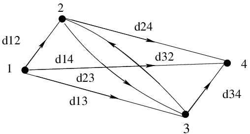
Consider the -node memoryless network depicted in Fig. 1 where each node has one message only. This model does not include broadcasting messages and was used in [15] and [21, Ch. 15] . Node , , has a message destined for nodes in the set , , while acting as a relay for messages of the other nodes. We write the set of nodes whose signals node must decode correctly as . The messages are mutually statistically independent and is uniformly distributed over the set , where is taken to be a non-negative integer.
The channel is described by the conditional probabilities
| (1) |
where and , , are the respective input and output alphabets, i.e., we have
If all alphabets are discrete and finite sets, then the network is called a discrete memoryless network (DMN) [22],[23, Ch.18]. As usual, we develop our random coding for DMNs and later extend the results to Gaussian channels. Node transmits at time and receives . The channel is memoryless and time invariant in the sense that
| (2) |
for all .
| Block | 1 | |||
|---|---|---|---|---|
| Multihop messages to nodes | ||||
| in channel uses | ||||
II-C Flooding
We can represent the DMN as a directed graph , where is a set of edges. Edges are denoted as . We label edge with the non-negative real number
| (3) |
called the capacity of the link, where is the mutual information between the random variables and conditioned on the event . Let be a path that starts from node and ends at node . Let to be the set of such paths. We write if lies on the path . We may communicate reliably between nodes and if
| (4) |
is positive. We assume that for all nodes with a message destined for node . Observe that if for all , then at most hops are needed for node to reliably convey its message at rate
| (5) |
by multihopping to all other nodes in the network. Hence, for a -node memoryless network at most hops are needed for all nodes to “flood” their messages by multihopping through the network.
Example 1

A line network with nodes is depicted in Fig. 2. Node has a message for node and we assume that , and so that node can communicate reliably to node by multihopping through nodes and with hops.
II-D Encoders and Decoders
We define two types of functions for each node :
- •
encoding functions that generate channel inputs based on the local message and past channel outputs
(6) - •
One decoding function
(7) where is the estimate of at node .
The average error probability for the network is defined as
| (8) |
A rate tuple is achievable for the DMN if for any , there is a sufficiently large integer and some functions and such that . The capacity region is the closure of the set of achievable rate tuples. For each node we define
| (9) |
where has the nodes whose messages node is not interested in but whose symbol sequences are included in the typicality test in order to remove interference. We further define, for any , the quantities
| (10) | ||||
| (11) |
III Main Result and Proof
The following theorem is the main result of this paper.
Theorem 1
For a -node memoryless network with one multicast session per node, SNNC with backward decoding achieves the same rate tuples as SNNC with sliding window decoding [5, 6] and LNNC with joint decoding [15, 14]. These are the rate tuples satisfying
| (12) |
for all , all subsets with and , where is the complement of in , and for joint distributions that factor as
| (13) |
Remark 1
The set (see (9)) represents the set of nodes whose messages are known or decoded at node . In other words, from node ’s perspective the network has nodes only.
Example 2
If , then the bound (12) is taken for all and all subsets with and , where is the complement of in .
Example 3
Consider and suppose node has a message destined for node , and node has a message destined
for node . We then have and . If nodes 3 and 4 choose and respectively, then we have and . In this case the rate bounds
(12) are:
Node :
| (14) | |||||
| (15) | |||||
Node :
| (16) |
III-A Encoding
To prove Theorem 1, we choose for all for simplicity. We later discuss the case where these sets are different. For clarity, we set the time-sharing random variable to be a constant. Table I shows the SNNC encoding process. We redefine to be the rate of the short messages in relation to the (redefined) block length . In other words, the message , of bits is split into equally sized blocks, , each of bits. Communication takes place over blocks and the true rate of will be
| (17) |
where is defined in (20) below.
Random Code: Fix a distribution . For each block and node , generate codewords , , according to where by convention. For each and , generate reconstructions , , according to . This defines the codebooks
| (18) | |||||
for and .
The codebooks used in the last blocks with are different. The blocks
| (19) |
are dedicated to flooding through the network, and for all nodes we generate independent and identically distributed (i.i.d.) codewords , , according to . We choose
| (20) |
that is independent of and . The overall rate of user is thus given by (17) which approaches as .
Encoding: Each node upon receiving at the end of block , , tries to find an index such that the following event occurs:
| (21) |
If there is no such index , set . If there is more than one, choose one. Each node transmits in block .
In the blocks (19), node conveys reliably to all other nodes by multihopping through the network with blocks of length .
III-B Backward Decoding
Let . At the end of block every node has reliably recovered via the multihopping of the last blocks.
For block , node tries to find tuples and such that the following event occurs:
| (22) |
where has already been reliably recovered from the previous block .
Error Probability: Let and assume without loss of generality that and . In each block , the error events at node are:
| (23) | ||||
| (24) | ||||
| (25) |
The error event at node in block thus satisfies
| (26) |
where we have used the union bound. can be made small with large , as long as (see [20])
| (27) |
where as . Similarly, can be made small with large .
To bound , for each and we define
| (28) | ||||
| (29) | ||||
| (30) |
and write . The important observations are:
- •
is independent of in the random coding experiment;
- •
The are mutually independent.
For and , we thus have
| (31) |
where as and
| (32) |
By the union bound, we have
| (33) |
where
- (a)
follows from (31)
- (b)
follows by collecting the into classes where
- (c)
follows because there are
(34) different that result in the same and such that , and
- (d)
is because for every node , we must have one of the following three cases occur:
- 1)
and
- 2)
and
- 3)
and
so there are different ways of choosing and .
- 1)
Since we require , we have
| (35) |
Combining (26), (27), (33) and (35) we find that we can make as if
| (36) |
for all subsets such that and . Of course, if , then we require that .
We can split the bounds in (36) into two classes:
| (37) | ||||
| (38) |
LNNC requires only the Class 1 bounds. SNNC requires both the Class 1 and Class 2 bounds to guarantee reliable decoding of the quantization indices for each backward decoding step. With the same argument as in [5, Sec. IV-C], we can show that the Class 2 bounds can be ignored when determining the best SNNC rates. SNNC with backward decoding thus performs as well as SNNC with sliding window decoding and LNNC with joint decoding.
IV Discussion
IV-A Sliding Window Decoding
SNNC with sliding window decoding was studied in [5, 6] and LNNC [15] achieves the same rates as in [5]. SNNC has extra constraints that turn out to be redundant [5, Sec. IV-C], [6, Sec. V-B]. The sliding window decoding in [5] resembles that in [24] where encoding is delayed (or offset) and different decoders are chosen depending on the rate point. The rates achieved by one decoder may not give the entire rate region of Theorem 1, but the union of achievable rates of all decoders does [6, Theorem 1]. The advantage of sliding window decoding is a small decoding delay of blocks as compared to backward decoding that requires blocks, where .
IV-B Backward Decoding
SNNC with backward decoding was studied in [7] for single source networks. For these networks, [7] showed that LNNC and SNNC achieve the same rates. Further, for a fixed random coding distribution there is a subset of the relay nodes whose messages should be decoded to achieve the best LNNC and SNNC rates. Several other interesting properties of the coding scheme were derived. It was also shown in [12] that SNNC with a layered network analysis [13] achieves the same LNNC rates for single source networks. In [25], SNNC with partial cooperation between the sources was considered for multi-source networks.
IV-C Multihopping
We compare how the approaches of Theorem 1 and [7, Theorem 2.5] reliably convey the last quantization indices . Theorem 1 uses multihopping while Theorem 2.5 in [7] uses a QF-style method with extra blocks after block with the same block length . In these blocks every node transmits as before except that the messages are set to a default value. The initialization method in [7] has two disadvantages:
- •
Both and must go to infinity to reliably decode [7, Sec.IV-A, Equ. (34)]. The true rate of node ’s message is
(39) and we choose so that as .
- •
Joint rather than per-block processing is used.
We remark that multihopping may be a better choice for reliably communicating , because the QF-style approach has a large decoding delay due to the large value of and does not use per-block processing.
IV-D Choice of Typicality Test


Theorem 1 has a subtle addition to [9] and difference to [15, Theorem 2] and[23, Theorem 18.5], namely that in (12) each may have a different set of nodes satisfying all Class constraints whose messages and quantization indices are included in the typicality test. But we can achieve the rates in (12) at node with SNNC by using backward decoding and treating the signals from the nodes in as noise. Hence we may ignore the Class constraints in (38) when determining the best SNNC rates.
The following example suggests that it may not be surprising that the SNNC and LNNC rate regions are the same. Consider the network in Fig. 3, where . Suppose both nodes 1 and 2 act as sources as well as relays for each other in transmitting information to node (see Fig. 3(a)). Referring to Theorem 1, the SNNC and LNNC bounds are (see Fig. 4):
| (40) | ||||
| (41) | ||||
| (42) |
However, suppose now that node 2 has no message () and acts as a relay node only (see Fig. 3(b)). Then LNNC does not have the bound (41) while SNNC has the bound (41) with and . We ask whether (41) reduces the SNNC rate. This is equivalent to asking whether SNNC achieves point in Fig. 4. It would be strange if there was a discontinuity in the achievable rate region at .
IV-E Joint Decoding
It turns out that SNNC with joint decoding achieves the same rates as in Theorem 1. Recently, the authors of [10] showed that SNNC with joint decoding fails to achieve the LNNC rates for a specific choice of SNNC protocol. However, by multihopping the last quantization indices and then performing joint decoding with the messages and remaining quantization bits, SNNC with joint decoding performs as well as SNNC with sliding window or backward decoding, and LNNC. This makes sense, since joint decoding should perform at least as well as backward decoding. Details are given in Appendix A.
IV-F Decoding Subsets of Messages
From Theorem 1 we know that if node decodes messages from nodes in and some of the Class constraints in (38) are violated, then we should treat the signals from the corresponding nodes as noise. In this way, we eventually wind up with some , , where all Class 2 constraints are satisfied, i.e., we have
| (43) |
and we achieve as good or better rates. In this sense, the sets are important even for LNNC. These sets seem difficult to find in large networks because many constraints need to be checked. However, provided that the sets are known, we have the following lemma.
Lemma 1

IV-G Optimal Decodable Sets
SNNC was studied for relay networks in [7]. For such networks there is one message at node that is destined for node . We thus have and . The authors of [7] showed that for a given random coding distribution
| (44) |
there exists a unique largest optimal decodable set , , of the relay nodes that provides the same best achievable rates for both SNNC and LNNC [7, Theorem 2.8]. We now show that the concept of optimal decodable set extends naturally to multi-source networks.
Lemma 2
For a -node memoryless network with a fixed random coding distribution
| (45) |
there exists for each node a unique largest set among all subsets satisfying (43). The messages of the nodes in should be included in the typicality test to provide the best achievable rates.
Proof:
We prove Lemma 2 without a time-sharing random variable . The proof with is similar. We show that is unique by showing that the union of any two sets and satisfying all constraints also satisfies all constraints and provides as good or better rates. Continuing taking the union, we eventually reach a unique largest set that satisfies all constraints and gives the best rates.
Partition the subsets into two classes:
Class : for all ;
Class : There exists one such that .
We may ignore the in Class because the proof of Theorem 1 shows that we can treat the signals of nodes associated with violated constraints as noise and achieve as good or better rates. Hence, we focus on in Class .
Suppose and are in Class and let . We define
| (46) | ||||
| (47) | ||||
| (48) |
Further, for every , define and . We have , , and . We further have
| (49) |
where
- (a)
follows from the definition of and
- (b)
follows because both and are in Class
- (c)
follows from the definition (10)
- (d)
follows because all are independent and conditioning does not increase entropy
- (e)
follows because conditioning does not increase entropy and by the Markov chains
(50) (51) - (f)
- (g)
follows from the definition (10).
The bound (49) shows that is also in Class . Moreover, by (49) if includes the messages of nodes in in the typicality test, then the rates are as good or better than those achieved by including the messages of nodes in or in the typicality test. Taking the union of all in Class , we obtain the unique largest set that gives the best achievable rates. ∎
Remark 2
There are currently no efficient algorithms for finding an optimal decodable set. Such algorithms would be useful for applications with time-varying channels.
V SNNC with a DF option
| Block | 1 | 2 | ||||
|---|---|---|---|---|---|---|
| Multihop | ||||||
| to node in | ||||||
| channel uses |
One of the main advantages of SNNC is that the relays can switch between QF (or CF) and DF depending on the channel conditions. If the channel conditions happen to be good, then the natural choice is DF which removes the noise at the relays. This not possible with LNNC due to the high rate of the long message. On the other hand, if a relay happens to experience a deep fade, then this relay should use QF (or CF).
In the following, we show how mixed strategies called SNNC-DF work for the multiple-relay channel. These mixed strategies are similar to those in [3, Theorem 4]. However, in [3] the relays use CF with a prescribed binning rate to enable step-by-step decoding (CF-S) instead of QF. In Section VI we give numerical examples to show that SNNC-DF can outperform DF, CF-S and LNNC.
As in [3], we partition the relays into two sets
where . The relays in use DF while the relays in use QF. Let be a permutation on with and and let , . Define . We have the following theorem.
Theorem 2
SNNC-DF achieves the rates satisfying
| (52) |
for all , where is the complement of in , and where the joint distribution factors as
| (53) |
Remark 3
As usual, we may add a time-sharing random variable to improve rates.
Proof:
For a given permutation and , the first mutual information term in (52) describes the DF bounds [3, Theorem 1] (see also [26, Theorem 3.1]). The second mutual information term in (52) describes the SNNC bounds. Using a similar analysis as for Theorem 1 and by treating as the “new” source signal at the destination, we have the SNNC bounds
| (54) | ||||
| (55) |
for all .
The same argument used to prove Theorem 1 shows that if any of the constraints (55) is violated, then we get rate bounds that can be achieved with SNNC-DF by treating the signals from the corresponding relay nodes as noise. Thus we may ignore the constraints (55). ∎
Example 4
If relay node 2 uses DF while relay node 3 uses CF-S, then by [3, Theorem 4] with , any rate up to
| (58) |
can be achieved, subject to
| (59) |
and the joint distribution factors as (57). It turns out that in (58)-(59) is the same as (56), since LNNC and SNNC do not improve the CF-S rate for one relay [8]. But is better than in general.
Remark 4
For rapidly changing channels it is advantageous to use independent inputs so all nodes can use the same encoder for all channel states. If and in the above example are independent, there is no need to use block Markov coding (BMC). However, we need to use two backward (or sliding window) decoders to recover the rates (56). See Appendix B.
Remark 5
How to perform DF for multiple sources is not obvious. Consider again the three node network in Fig. 3, but now every node wishes to send a message to the other two nodes. How should one set up cooperation if all nodes may use DF? Such questions are worth addressing, since their answers will give insight on how to incorporate mixed strategies to boost system performance.
VI Gaussian Networks
We next consider additive white Gaussian noise (AWGN) networks. We use to denote a circularly symmetric complex Gaussian random variable with mean and variance . Let be a noise string whose symbols are i.i.d. and for all . The channel output at node is
| (60) |
where the channel gain is
| (61) |
and is the distance between nodes and , is a path-loss exponent and is a complex fading random variable.
We consider two kinds of fading:
- •
No fading: is a constant and known at all nodes. We set for all .
- •
Rayleigh fading: we have . We assume that a destination node knows for all and a relay node knows for all and knows the statistics of all other . We focus on slow fading, i.e., all remain unchanged once chosen.
We avoid issues of power control by imposing a per-symbol power constraint . We choose the inputs to be Gaussian, i.e., , .
In the following we give numerical examples for four different channels
- •
the relay channel;
- •
the two-relay channel;
- •
the multiple access relay channel (MARC);
- •
the two-way relay channel (TWRC).
We evaluate the performance for no fading in terms of achievable rates (in bits per channel use) and for Rayleigh fading in terms of outage probability [27] for a target rate .
Relay node chooses
| (62) |
where . For the no fading case, relay node numerically calculates the optimal for CF-S and SNNC, and the optimal binning rate for CF-S, in order to maximize the rates. For DF, the source and relay nodes numerically calculate the power allocation for superposition coding that maximizes the rates. For the Rayleigh fading case, relay node knows only the , , but it can calculate the optimal and based on the statistics of , for all so as to minimize the outage probability. For DF, the fraction of power that the source and relay nodes allocate for cooperation is calculated numerically based on the statistics of , for all , to minimize the outage probability. Details of the derivations are given in Appendix C.
VI-A Relay Channels


VI-A1 No Fading
Fig. 5 depicts the geometry and Fig. 6 depicts the achievable rates as a function of for and . DF achieves rates close to capacity when the relay is close to the source while CF-S dominates as the relay moves towards the destination. For the relay channel, CF-S performs as well as SNNC (LNNC). SNNC-DF unifies the advantages of both SNNC and DF and achieves the best rates for all relay positions.
VI-A2 Slow Rayleigh fading
Fig. 7 depicts the outage probabilities with , , , and .

Over the entire power range CF-S gives the worst outage probability. This is because CF-S requires a reliable relay-destination link so that both the bin and quantization indices can be recovered. Both DF and SNNC improve on CF-S. DF performs better at low power while SNNC is better at high power. SNNC-DF has the relay decode if possible and perform QF otherwise, and gains dB over SNNC and DF.
VI-B Two-Relay Channels
The Gaussian two-relay channel (Fig. 8) has
| (65) | ||||
| (66) | ||||
| (67) |
where the relay nodes and help node transmit a message to node .
VI-B1 No Fading
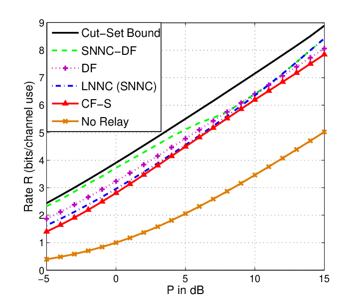
The CF-S rates are the lowest over the entire power range. As expected, SNNC improves on CF-S. DF performs better than SNNC at low power but worse at high power. SNNC-DF achieves the best rates and exhibits reasonable rate and power gains over SNNC and DF for to . The gains are because in this power range SNNC-DF has relay 2 performing DF and relay 3 performing QF.
VI-B2 Slow Rayleigh Fading

CF-S gives the worst performance over the entire power range. This is because CF-S requires a reliable relay-destination link for both relays so that the bin and quantization indices for both relays can be decoded. DF provides better outage probabilities than CF-S but is worse than SNNC or LNNC, since it requires reliable decoding at both relays. SNNC-DF has the two relays decode if possible and perform QF otherwise and gains about dB over LNNC (SNNC). In general, we expect larger gains of SNNC-DF over LNNC for networks with more relays.
VI-C Multiple Access Relay Channels
VI-C1 No Fading
Fig. 11 depicts the geometry and Fig. 12 depicts the achievable rate regions for , dB and . The SNNC rate region includes the CF-S rate region. Through time-sharing, the SNNC-DF region is the convex hull of the union of DF and SNNC regions. SNNC-DF again improves on LNNC (or SNNC) and DF.


VI-C2 Slow Rayleigh Fading
Fig. 13 depicts the outage probabilities with , , , , , and .

CF-S has the worst outage probability because it requires a reliable relay-destination link to decode the bin and quantization indices. DF has better outage probability than CF-S, while LNNC (or SNNC) improves on DF over the entire power range. SNNC-DF has the relay perform DF or QF depending on channel quality and gains dB at low power and dB at high power over SNNC.
Remark 6
The gain of SNNC-DF over SNNC is not very large at high power. This is because the MARC has one relay only. For networks with more relays we expect larger gains from SNNC-DF.
VI-D Two-Way Relay Channels
The Gaussian TWRC (Fig. 14) has
| (70) | ||||
| (71) | ||||
| (72) |
where nodes 1 and 2 exchange messages with the help of relay node 3.

VI-D1 No Fading
Fig. 14 depicts the geometry and Fig. 15 depicts the achievable sum rates for and . DF gives the best rates at low power while SNNC provides better rates at high power. The CF-S rates are slightly lower than the SNNC rates over the entire power range. SNNC-DF combines the advantages of SNNC and DF and achieves the best rates throughout.

VI-D2 Slow Rayleigh Fading

CF-S has the worst outage probability since it requires that both relay-destination links () are reliable so that the bin and quantization indices can be recovered at both destinations and . DF is better than CF-S, while LNNC (or SNNC) improves on DF. SNNC-DF lets the relay use DF or QF depending on the channel conditions and gains over about dB at low power and dB at high power over LNNC (or SNNC).
VII Concluding Remarks
SNNC enables early decoding at nodes, and this enables the use of SNNC-DF. Numerical examples demonstrate that SNNC-DF shows reasonable gains as compared to DF, CF-S and LNNC in terms of rates and outage probabilities.
Appendix A SNNC with joint Decoding
After block every node can reliably recover via the multihopping of the last blocks.
Let . Node tries to find a and such that the event (22) occurs for all , where is already known. The difference between joint decoding and backward decoding is that the typicality test is performed jointly over all blocks (see (73)-(75) below) while it is performed in only one block in (23)-(25).
Error Probability: Let . Assume without loss of generality that and for . For any , define
The error events at decoder are:
| (73) | ||||
| (74) | ||||
| (75) |
The error event at node thus satisfies
| (76) |
where we have used the union bound.
| Block | 1 | 2 | |||
|---|---|---|---|---|---|
can be made small with large as long as (see (27))
| (77) |
Also, we have
| (78) |
where follows because , which goes to zero as , for [20].
To bound , for each , we define
| (79) |
and write . Observe that for
- •
is independent of in the random coding experiment;
- •
the are mutually independent.
| (80) |
where
and as .
By the union bound, we have
| (83) |
where
Performing the same steps as in (35) and (36), we require
| (85) |
for all subsets such that and . We can again split the bounds in (85) into two classes:
| (86) | ||||
| (87) |
and show that the constraints in (87) at node are redundant with the same argument used for backward decoding. By the union bound, the error probability for all destinations tends to zero as if the rate tuple satisfies (12) for all subsets such that and and for any joint distribution that factors as (13).
Appendix B Backward Decoding for the Two-Relay Channel without Block Markov Coding
The coding scheme is the same as in Example 4, except that no BMC is used (see Table III). We show how to recover the rate (56) with independent inputs and with different backward decoders.
Decoding at Relays:
Node . For , node 2 tries to find a that satisfies
| (88) |
Node 2 can reliably decode if
| (89) |
where as (see [20]).
Backward Decoding at the destination: Let .
Decoder 1:
Multihop to node in blocks to .
For , node declares , if there is a unique pair satisfying the following typicality checks in both blocks and :
| (92) |
and
| (93) |
where and have already been reliably decoded from the previous block .
Similar analysis as in Theorem 1 shows that node 4 can reliably recover if
| (94) | ||||
| (95) | ||||
| (96) |
If the constraint (96) is violated, then the rate bound (95) becomes
| (97) |
which is a stronger bound than (94) and can be achieved with SNNC-DF by treating as noise. Thus, we may ignore (96).
Decoder 2:
Multihop and to node in blocks to .
For , node 4 declares , if there is a unique pair satisfying the following typicality checks in both blocks and :
| (98) | ||||
| (99) |
and
| (100) |
where , and have already been reliably decoded from the previous block .
Node can reliably recover if
| (101) | ||||
| (102) | ||||
| (103) |
If the constraint (103) is violated, then the rate bound (102) becomes
| (104) |
and the resulting can be achieved by using decoder (see (94)). Thus, with the combination of both decoders, we may ignore (103) and achieve the rate (56).
Remark 7
Sliding window decoding with 2 different decoders also recovers the rate (56) for independent and and enjoys a smaller decoding delay.
Appendix C Rates and Outage for Gaussian Networks
In the following, let , .
C-A Relay Channels
C-A1 No Fading
The achievable rates with DF and CF-S are given in [3]. The SNNC and LNNC rates are simply the CF-S rate. The SNNC-DF rate is the larger of the SNNC and DF rates.
C-A2 Slow Rayleigh Fading
Define the events
| (105) |
where is the fraction of power allocated by source to sending new messages. The optimal , and are calculated numerically.
The DF, CF-S, SNNC and SNNC-DF rates are
where
and is the real part of and is the complex conjugate of .
Remark 8
For SNNC, event means that
| (114) |
and the destination can reliably recover and jointly which helps to decode . Otherwise the destination should treat as noise to get a better rate (see Theorem 1). Similarly, for CF-S the events and mean that both and can be decoded in a step-by-step fashion [1]. If and occur, then can be recovered which removes interference at the receiver. Otherwise the relay signal should be treated as noise.
As recognized in [28], one drawback of DF is that if the source-relay link happens to be weak and the relay tries to decode, then the rate suffers. Hence the relay should decode only if the source-relay link is strong enough to support , i.e., if event occurs. Otherwise, the relay should perform CF-S or QF. Different choices of relay operations depending on the channel conditions lead to the achievable rates with SNNC-DF.
The outage probabilities are as follows:
| (115) |
C-B Two-Relay Channels
C-B1 No Fading
The achievable DF rates are [3, Theorem 1]
| (116) |
where
| (117) |
with
| (118) |
where and and the optimal power allocation parameters are calculated numerically.
The CF-S rates are (see [3, Theorem 2] with , )
| (119) |
subject to
where
| (120) |
The optimal and are calculated numerically.
Referring to Theorem 1, the achievable SNNC rates are
| (121) |
where
| (122) |
where is defined in (120). The optimal and are calculated numerically.
If one relay uses DF and the other uses QF, rates satisfying
| (123) |
can be achieved, where
with
| (124) |
and
| (125) |
where and the optimal , and for and are calculated numerically.
Referring to Theorem 2, SNNC-DF achieves rates satisfying
| (126) |
C-B2 Slow Rayleigh Fading
Define the events
| (138) |
where takes on the value or (see (118)) and the choice depends on the statistics of the fading coefficients such that the DF outage probability is minimized.
The DF rates are
| (139) |
The CF-S rates are
where is defined in (120) and
| (143) |
Observe that if both and occur, then both the bin and quantization indices can be decoded. If only occurs, then only the bin index can be recovered.
Referring to Theorem 1 the SNNC rates are
where
| (148) |
The event means that both quantization indices can be recovered. The events and mean that only one of the two quantization indices can be decoded.
C-C Multiple Access Relay Channels
C-C1 No Fading
The DF rate region of the Gaussian MARC is the union of all pairs satisfying [29, Sec. 3]
| (153) |
where
| (154) |
where and . The optimal power allocation parameters are calculated numerically.
The achievable CF-S rate region is the union of all pairs satisfying [29, Sec. 3]
| (155) |
where
| (156) |
for some
C-C2 Slow Rayleigh Fading
Define the events
| (161) |
The DF rate region of the Gaussian MARC is the union of all rate pairs satisfying (153). The CF-S rate region is the union of all satisfying [29]
where
| (171) |
If both and occur, then the relay bin and quantization indices can be decoded. If only occurs, then only the bin index can be recovered.
Referring to Theorem 1, the SNNC rate region is the union of all pairs satisfying
The event means that the destination should decode the relay signal to achieve better performance.
The SNNC-DF rate region is the union of all satisfying
If occurs, then the relay should decode which will remove interference at the relay. Otherwise, the relay should perform QF to avoid unnecessarily lowering the rates.
Let . The outage probabilities are:
| (184) |
C-D Two-Way Relay Channels
C-D1 No Fading
The DF rate region for the Gaussian TWRC is the union of all satisfying
| (185) |
where
| (186) |
where and . The optimal power allocation parameters are calculated numerically.
Referring to Theorem 1, the SNNC rate region is the union of all satisfying
| (188) |
where
for some . The SNNC-DF rate region is the union of the DF and SNNC rate regions.
C-D2 Slow Rayleigh Fading
Define the events
The DF region is the union of all satisfying (185). The CF-S region is the union of all satisfying
where
The optimal and are calculated numerically.
Referring to Theorem 1, SNNC achieves all pairs satisfying
The SNNC-DF rate region is the union of the satisfying
The outage probabilities are:
| (203) |
References
- [1] T. Cover and A. E. Gamal, “Capacity theorems for the relay channel,” IEEE Trans. Inf. Theory, vol. 25, no. 5, pp. 572–584, Sept. 1979.
- [2] B. Schein, “Distributed coordination in network information theory,” Ph.D. dissertation, MIT, Cambridge, MA, USA, 2001.
- [3] G. Kramer, M. Gastpar, and P. Gupta, “Cooperative strategies and capacity theorems for relay networks,” IEEE Trans. Inf. Theory, vol. 51, no. 9, pp. 3037–3063, Sept. 2005.
- [4] M. Yassaee and M. Aref, “Generalized compress-and-forward strategy for relay networks,” in IEEE Int. Symp. Inf. Theory, Toronto, Canada, July 2008, pp. 2683–2687.
- [5] ——, “Slepian-Wolf coding over cooperative networks,” in IEEE Int. Symp. Inf. Theory, Seoul, Korea, June 2009, pp. 879–883.
- [6] ——, “Slepian-Wolf coding over cooperative relay networks,” IEEE Trans. Inf. Theory, vol. 57, no. 6, pp. 3462–3482, 2011.
- [7] X. Wu and L.-L. Xie, “On the optimal compressions in the compress-and-forward relay schemes,” IEEE Trans. Inf. Theory, vol. 59, no. 5, pp. 2613–2628, 2013.
- [8] G. Kramer and J. Hou, “Short-message quantize-forward network coding,” in 2011 8th Int. Workshop on Multi-Carrier Systems Solutions (MC-SS), Herrsching, Germany, May 2011, pp. 1–3.
- [9] ——, “On message lengths for noisy network coding,” in IEEE Inf. Theory Workshop (ITW), Paraty, Brazil, Oct. 2011, pp. 430–431.
- [10] P. Zhong, A. Haija, and M. Vu, “On compress-forward without Wyner-Ziv binning for relay networks,” submitted to IEEE Trans. Inf. Theory, 2011. [Online]. Available: http://arxiv.org/abs/1111.2837/
- [11] J. Hou and G. Kramer, “Short message noisy network coding for multiple sources,” in IEEE Int. Symp. Inf. Theory, Boston, USA, July 2012, pp. 1677–1681.
- [12] A. Raja and P. Viswanath, “Compress-and-forward scheme for a relay network: Approximate optimality and connection to algebraic flows,” submitted to IEEE Trans. Inf. Theory, June 2012. [Online]. Available: http://arxiv.org/abs/1012.0416/
- [13] A. Avestimehr, S. Diggavi, and D. Tse, “Wireless network information flow: A deterministic approach,” IEEE Trans. Inf. Theory, vol. 57, no. 4, pp. 1872–1905, April 2011.
- [14] S. Lim, Y.-H. Kim, A. El Gamal, and S.-Y. Chung, “Noisy network coding,” in Inf. Theory Workshop (ITW), Cairo, Egypt, Jan. 2010, pp. 1–5.
- [15] ——, “Noisy network coding,” IEEE Trans. Inf. Theory, vol. 57, no. 5, pp. 3132–3152, May 2011.
- [16] R. Ahlswede, N. Cai, S.-Y. Li, and R. Yeung, “Network information flow,” IEEE Trans. Inf. Theory, vol. 46, no. 4, pp. 1204–1216, July 2000.
- [17] A. Dana, R. Gowaikar, R. Palanki, B. Hassibi, and M. Effros, “Capacity of wireless erasure networks,” IEEE Trans. Inf. Theory, vol. 52, no. 3, pp. 789–804, March 2006.
- [18] N. Ratnakar and G. Kramer, “The multicast capacity of deterministic relay networks with no interference,” IEEE Trans. Inf. Theory, vol. 52, no. 6, pp. 2425–2432, June 2006.
- [19] J. L. Massey, Applied Digital Information Theory, ETH Zurich, Zurich, Switzerland, 1980-1998.
- [20] A. Orlitsky and J. Roche, “Coding for computing,” IEEE Trans. Inf. Theory, vol. 47, no. 3, pp. 903–917, March 2001.
- [21] T. Cover and J. Thomas, Elements of Information Theory, 2nd ed. New York: Wiley, 2006.
- [22] G. Kramer, “Capacity results for the discrete memoryless network,” IEEE Trans. Inf. Theory, vol. 49, no. 1, pp. 4–21, Jan. 2003.
- [23] A. El Gamal and Y.-H. Kim, Network Information Theory. Cambridge University Press, 2011.
- [24] L. Sankar, G. Kramer, and N. B. Mandayam, “Offset encoding for multiple-access relay channels,” IEEE Trans. Inf. Theory, vol. 53, no. 10, pp. 3814–3821, 2007.
- [25] J. Du, M. Xiao, M. Skoglund, and S. Shamai (Shitz), “Short-message noisy network coding with partial source cooperation,” in Inf. Theory Workshop (ITW), Lausanne, Switzerland, Sept. 2012, pp. 144–147.
- [26] L.-L. Xie and P. Kumar, “An achievable rate for the multiple-level relay channel,” IEEE Trans. Inf. Theory, vol. 51, no. 4, pp. 1348–1358, April 2005.
- [27] L. Ozarow, S. Shamai, and A. Wyner, “Information theoretic considerations for cellular mobile radio,” IEEE Trans. on Veh. Technol., vol. 43, no. 2, pp. 359–378, May 1994.
- [28] J. Laneman, D. Tse, and G. Wornell, “Cooperative diversity in wireless networks: Efficient protocols and outage behavior,” IEEE Trans. Inf. Theory, vol. 50, no. 12, pp. 3062–3080, Dec. 2004.
- [29] L. Sankaranarayanan, G. Kramer, and N. Mandayam, “Hierarchical sensor networks: capacity bounds and cooperative strategies using the multiple-access relay channel model,” in 2004 First Annual IEEE Commun. Soc. Conf. on Sensor and Ad Hoc Commun. and Networks, Santa Clara, Oct. 2004, pp. 191–199.
- [30] B. Rankov and A. Wittneben, “Achievable rate regions for the two-way relay channel,” in IEEE Int. Symp. Inf. Theory, Seattle, USA, July 2006, pp. 1668–1672.