On Hodges and Lehmann’s “6/ Result"
Abstract
While the asymptotic relative efficiency (ARE) of Wilcoxon rank-based tests for location and regression with respect to their parametric Student competitors can be arbitrarily large, Hodges and Lehmann (1961) have shown that the ARE of the same Wilcoxon tests with respect to their van der Waerden or normal-score counterparts is bounded from above by . In this paper, we revisit that result, and investigate similar bounds for statistics based on Student scores. We also consider the serial version of this ARE. More precisely, we study the ARE, under various densities, of the Spearman-Wald-Wolfowitz and Kendall rank-based autocorrelations with respect to the van der Waerden or normal-score ones used to test (ARMA) serial dependence alternatives.
Keywords:
Asymptotic relative efficiency, rank-based tests, Wilcoxon test, van der Waerden test, Spearman autocorrelations, Kendall autocorrelations, linear serial rank statistics1 Introduction
The Pitman asymptotic relative efficiency under density of a test with respect to a test is defined as the limit (when it exists) as tends to infinity of the ratio of the number of observations it takes for the test , under density , to match the local performance of the test based on observations. That concept was first proposed by Pitman in the unpublished lecture notes [28] he prepared for a 1948-49 course at Columbia University. The first published rigorous treatment of the subject was by Noether [25] in 1955. A similar definition applies to point estimation; see, for instance, [6] for a more precise definition. An in-depth treatment of the concept can be found in Chapter 10 of Serfling [31], Chapter 14 of van der Vaart [32], or in the monograph by Nikitin [24].
The study of the AREs of rank tests and R-estimators with respect to each other or with respect to their classical Gaussian counterparts has produced a number of interesting and sometimes surprising results. Considering the van der Waerden or normal-score two-sample location rank test and its classical normal-theory competitor, the two-sample Student test , Chernoff and Savage in 1958 established the rather striking fact that, under any density satisfying very mild regularity assumptions,
| (1.1) |
with equality holding at the Gaussian density only. That result implies that rank tests based on Gaussian scores (that is, the two-sample rank-based tests for location, but also the one-sample signed-rank ones, traditionally associated with the names of van der Waerden, Fraser, Fisher, Yates, Terry and/or Hoeffding—for simplicity, in the sequel, we uniformly call them van der Waerden tests—asymptotically outperform the corresponding everyday practice Student -test; see [1]. That result readily extends to one-sample symmetric and -sample location, regression and analysis of variance models with independent noise.
Another celebrated bound is the one obtained in 1956 by Hodges and Lehmann, who proved that, denoting by the Wilcoxon test (same location and regression problems as above),
| (1.2) |
which implies that the price to be paid for using rank- or signed-rank tests of the Wilcoxon type (that is, logistic-score-based rank tests) instead of the traditional Student ones never exceeds 13.6% of the total number of observations. That bound moreover is sharp, being reached under the Epanechnikov density . On the other hand, the benefits of considering Wilcoxon rather than Student can be arbitrarily large, as it is easily shown that the supremum over of is infinite; see [20].
Both (1.1) and (1.2) created quite a surprise in the statistical community of the late fifties, and helped dispelling the wrong idea, by then quite widespread, that rank-based methods, although convenient and robust, could not be expected to compete with the efficiency of traditional parametric procedures.
Chernoff-Savage and Hodges-Lehmann inequalities since then have been extended to a variety of more general settings. In the elliptical context, optimal rank-based procedures for location (one and -sample case), regression, and scatter (one and -sample cases) have been constructed in a series of papers by Hallin and Paindaveine ([7], [11], and [13]), based on a multivariate concept of signed ranks. The Gaussian competitors here are of the Hotelling, Fisher, or Lagrange multiplier forms. For all those tests, Chernoff-Savage result similar to (1.1) have been established (see also [26, 27]). Hodges-Lehmann results also have been obtained, with bounds that, quite interestingly, depend on the dimension of the observation space: see [7].
Another type of extension is into the direction of time series and linear rank statistics of the serial type. Hallin [5] extended Chernoff and Savage’s result (1.1) to the serial context by showing that the serial van der Waerden rank tests also uniformly dominate their Gaussian competitors (of the correlogram-based portmanteau, Durbin-Watson or Lagrange multiplier forms). Similarly, Hallin and Tribel [19] proved that the 0.864 upper bound in (1.2) no longer holds for the AREs of the Wilcoxon serial rank test with respect to their Gaussian competitors, and is to be replaced by a slightly lower 0.854 one. Elliptical versions of those results are derived in Hallin and Paindaveine ([8], [9], [10]).
Now, AREs with respect to Gaussian procedures such as -tests are not always the best evaluations of the asymptotic performances of rank-based tests. Their existence indeed requires the Gaussian procedures to be valid under the density under consideration, a condition which places restrictions on that may not be satisfied. When the Gaussian tests are no longer valid, one rather may like to consider AREs of the form
| (1.3) |
comparing the asymptotic performances (under ) of two rank-based tests and , based on score-generating functions and , respectively. Being distribution-free, rank-based procedures indeed do not impose any validity conditions on , so that in general exists under much milder requirements on ; see, for instance, [17] and [18], where AREs of the form (1.3) are provided for rank-based methods in linear models with stable errors under which Student tests are not valid.
Obtaining bounds for ARE, in general, is not as easy as for AREs of the form ARE. The first result of that type was established in 1961 by Hodges and Lehmann, who in [21] show that
| (1.4) |
or, equivalently,
| (1.5) |
for all in some class of density functions satisfying weak differentiability conditions. Hodges and Lehmann moreover exhibit a parametric family of densities for which the function achieves any value in the open interval ( achieves any value in the open interval ). The lower and upper bounds in (1.4) and (1.5) thus are sharp in the sense that they are the best possible ones. The same result was extended and generalized by Gastwirth [2].
Note that, in case has finite second-order moments (so that is well defined), since , Hodges and Lehmann’s “ result" implies that the ARE of the van der Waerden tests with respect to the Student ones, which by the Chernoff-Savage inequality is larger than or equal to one, actually can be arbitrarily large, and that this happens for the same types of densities as for the Wilcoxon tests. This is an indication that, when Wilcoxon is quite significantly outperforming Student, that performance is shared by a broad class of rank-based tests and -estimators, which includes the van der Waerden ones.
In Section 2, we successively consider the traditional case of nonserial rank statistics used in the context of location and regression models with independent observations, and the case of serial rank statistics; the latter involve ranks at time and , say, and aim at detecting serial dependence among the observations. Serial rank statistics typically involve two score functions and, instead of (1.3), yield AREs of the form
| (1.6) |
To start with, in Section 2.1, we revisit Gastwirth’s classical nonserial results. More precisely, we provide (Proposition 2.2) a slightly different proof of the main proposition in [2], with some further illustrations in the case of Student scores. In Section 2.2, we turn to the serial case, with special attention for the so-called Wilcoxon-Wald-Wolfowitz, Kendall and van der Waerden rank autocorrelation coefficients. Serial AREs of the form (1.6) typically are the product of two factors to which the nonserial techniques of Section 2.1 separately apply; this provides bounds which, however, are not sharp. Therefore, in Section 3, we restrict to a few parametric families—the Student family (indexed by the degrees of freedom), the power-exponential family, or the Hodges-Lehmann family —for which numerical values are displayed.
2 Asymptotic relative efficiencies of rank-based procedures
The asymptotic behavior of rank-based test statistics under local alternatives, since Hájek and Šidák [4], is obtained via an application of Le Cam’s Third Lemma (see, for instance, Chapter 13 of [32]). Whether the statistic is of the serial or the nonserial type, the result, under a density with distribution function involves integrals of the form
and, in the serial case,
where, assuming that admits a weak derivative , is such that the Fisher information for location is finite. Denote by the class of such densities. If local alternatives, in the serial case, are of the ARMA type, is further restricted to the subset of densities having finite second-order moments. Differentiability in quadratic mean of is the standard assumption here, see Chapter 7 of [32]; but absolute continuity of in the traditional sense, with a.e. derivative , is sufficient for most purposes. We refer to [4] and [16] for details in the nonserial and the serial case, respectively.
2.1 The nonserial case
In location or regression problems, or, more generally, when testing linear constraints on the parameters of a linear model (this includes ANOVA etc.), the ARE, under density , of a rank-based test based on the square-summable score-generating function with respect to another rank-based test based on the square-summable score-generating function takes the form
| (2.1) |
provided that and are monotone, or the difference between two monotone functions. Those ARE values readily extend to the -sample setting, and to R-estimation problems. In a time-series context with innovation density , and under slightly more restrictive assumptions on the scores, they also extend to the partly rank-based tests and R-estimators considered by Koul and Saleh in [22] and [23].
Gastwirth (1970) is basing his analysis of (2.1) on an integration by parts of the integral in the definition of . If both and are differentiable, with derivatives and , respectively, and provided that is such that
integration by parts in those integrals yields, for (2.1),
| (2.2) |
In view of the Chernoff-Savage result (1.1), the van der Waerden score-generating function
| (2.3) |
(with the standard normal quantile function) may appear as a natural benchmark for ARE computations. From a technical point of view, under this integration by parts approach, the Wilcoxon score-generating function
| (2.4) |
(the Spearman-Wald-Wolfowitz score-generating function in the serial case) is more appropriate, though. Convexity arguments indeed will play an important role, and, being linear, is both convex and concave. Since and , equation (2.2) yields
| (2.5) |
Bounds on then readily yield bounds on AREs, irrespective of .
That property of Wilcoxon scores is exploited in Propositions 2.2 and 2.3 for non-serial AREs, in Propositions 2.4 for the serial ones; those bounds are mainly about AREs of, or with respect to, Wilcoxon (Spearman-Wald-Wolfowitz) procedures, but not exclusively so.
Assume that . Then, integration by parts is possible in the definition of , yielding
Assume furthermore that the square-integrable score-generating function (the difference of two monotone increasing functions) is differentiable, with derivative , and that
so that (2.2) holds. Finally, assume that is skew-symmetric about . Defining the (possibly infinite) constants
we can always write
| (2.6) |
while, if is non-decreasing (hence is non-negative), we further have
| (2.7) |
The quantities appearing in (2.6) and (2.7) often can be computed explicitly, yielding ARE bounds which are, moreover, sharp under certain conditions (see below).
For example, if is convex on , its derivative is non-decreasing over , so that
| (2.8) |
It follows that, under the assumptions made,
| (2.9) |
The lower bound in (2.9) is established in Theorem 2.1 of [2].
The double inequality (2.9) holds, for instance (still, under ), when the scores are the optimal scores associated with some symmetric and strongly unimodal density with distribution function ; such densities indeed are log-concave and have monotone increasing, convex over score functions. Symmetric log-concave densities take the form
| (2.10) |
with a convex, even (that is, ) function; assume it to be twice differentiable, with derivatives and . Then, , so that
where the Fisher information of (which we assume to be finite), and
Specializing (2.9) to this situation, we obtain the following proposition.
Proposition 2.1.
If the square-integrable score-generating function is of the form with given by (2.10), even, convex, and twice differentiable, then, under any ,
| (2.11) |
With (so that ) in (2.10), is the standard Gaussian density; , , and the lower bound in (2.11 ) becomes , whereas the upper bound is trivially infinite. This yields the Hodges-Lehmann result (1.4).
Turning back to (2.6) and (2.7), but with concave (and still non-decreasing) on , is nonincreasing, so that and
| (2.12) |
Not much can be said on the lower bound, though, without further assumptions on the behavior of around .
Replacing, for various score-generating functions and densities , the quantities appearing in (2.6), (2.9) or (2.12) with their explicit values provides a variety of bounds of the Hodges-Lehmann type. Below, we consider the van der Waerden tests , based on the score-generating function (2.3) and the Cauchy-score rank tests , based on the score-generating function
| (2.13) |

Proposition 2.2.
For all symmetric densities in , and , respectively,
- (i)
;
- (ii)
;
- (iii)
.
Proof.
The van der Waerden score (2.3) is strictly increasing, and convex over . One readily obtains
hence . Plugging this into the left-hand side inequality of (2.9) yields (i). Alternatively one can directly apply (2.11).
The Cauchy score is concave over , but not monotone (being of bounded variation, however, it is the difference of two monotone function). Direct inspection of (2.13) nevertheless reveals that
hence . Substituting this in (2.6) yields (ii). The product of the upper bounds in (i) and (ii) yields (iii). ∎
Remarkably, those three bounds are sharp. Indeed, numerical evaluation shows that they can be approached arbitrarily well by taking extremely heavy-tails such as those of stable densities with tail index , Student densities with degrees of freedom , or Pareto densities with ; see also the family of densities Ê defined inÊ equation (3.1).
Figure 1 provides plots of and for various densities. Inspection of those graphs shows that both AREs are decreasing as the tails become lighter; the sharpness of bounds (i) and (iii), hence also that of bound (ii), is graphically confirmed.
The bounds proposed in Proposition 2.2 are not new, and have been obtained already in [2]. One would like to see similar bounds for other score functions, such as the Student ones
| (2.14) | |||||
where denotes the inverse of the regularized incomplete beta function evaluated at and stands for the Student quantile function with degrees of freedom. Note that , so that . Since and , this means that, on , is a redescending function; in general, it is neither convex nor concave on .
Differentiating (2.14), we get, for ,
| (2.15) |
from which we deduce that
Except for the case, which is covered by (ii) and (iii) in Proposition 2.2, these values do not provide exploitable values for . For , however, one can check from (2.15) that , so that
Elementary though somewhat tedious algebra yields
Plugging this into (2.6), we obtain, for , the following additional bounds.
Proposition 2.3.
For all and all symmetric density in and , respectively,
- (iv)
, and
- (v)
.
Inequality (iv) is sharp, the bound being achieved, in the limit, under very heavy tails (stable densities with , or Student- densities with ). Since this is also the case, under the same sequences of densities, for inequality (i) in Proposition 2.1, inequality (v) is sharp as well. The upper bounds (iv) and (v) are both decreasing functions of the tail index ; both are unbounded at the origin, and both converge to the corresponding Cauchy values as .
2.2 The serial case
Until the early eighties, and despite some forerunning time-series applications such as Wald and Wolfowitz [33] (published as early as 1943—two years before Frank Wilcoxon’s pathbreaking 1945 paper [34]!), rank-based methods had been essentially limited to statistical models involving univariate independent observations. Therefore, the traditional ARE bounds (Hodges and Lehmann [20, 21], Chernoff-Savage [1] or Gastwirth [2]), as well as the classical monographs (Hájek and Šidák [4], Randles and Wolfe [30], Puri and Sen [29], to quote only a few) mainly deal with univariate location and single-output linear (regression) models with independent observations. The situation since then has changed, and rank-based procedures nowadays have been proposed for a much broader class of statistical models, including time series problems, where serial dependencies are the main features under study.
In this section, we focus on the linear rank statistics of the serial type involving two square-integrable score functions. Those statistics enjoy optimality properties in the context of linear time series (ARMA models; see [16] for details). Once adequately standardized, those statistics yield the so-called rank-based autocorrelation coefficients. Denote by the ranks in a triangular array of observations. Rank autocorrelations (with lag ) are linear serial rank statistics of the form
where and are (square-integrable) score-generating functions, whereas and denote the exact mean of and the exact standard error of under the assumption of i.i.d. ’s (more precisely, exchangeable ’s), respectively; we refer to pages 186 and 187 of [16] for explicit formulas. Signed-rank autocorrelation coefficients are defined similarly; see [15] or [16].
Rank and signed-rank autocorrelations are measures of serial dependence offering rank-based alternatives to the usual autocorrelation coefficients, of the form
which consitute the Gaussian reference benchmark in this context. Of particular interest are
- (i)
the van der Waerden autocorrelations [14]
- (ii)
the Wald-Wolfowitz or Spearman autocorrelations [33]
- (iii)
and the Kendall autocorrelations [3] (where explicit values of and are provided)
with denoting the number of discordances at lag , that is, the number of pairs and that satisfy either
more specifically,
The van der Waerden autocorrelations are optimal—in the sense that they allow for locally optimal rank tests in the case of ARMA models with normal innovation densities. The Spearman and Kendall autocorrelations are serial versions of Spearman’s rho and Kendall’s tau, respectively, and are asymptotically equivalent under the null hypothesis of independence; although they are never optimal for any ARMA alternative, they achieve excellent overall performance. Signed rank autocorrelations are defined in a similar way.
Let , denote four square-summable score functions, and assume that they are monotone increasing, or the difference between two monotone increasing functions (that assumption tacitly will be made in the sequel each time AREs are to be computed). Recall that denotes the subclass of densities having finite moments of order two. The asymptotic relative efficiency, under innovation density , of the rank-based tests based on the autocorrelations with respect to the rank-based tests based on the autocorrelations is
| (2.16) |
with and .
The ratios have been studied in Section 2.1, and the same conclusions apply here; as for the ratios, they can be treated by similar methods.
Denote by , , , the tests based on, , , etc. The serial counterpart of is , for which the following result holds.
Proposition 2.4.
Let the score functions and be monotone increasing, skew-symmetric about , and differentiable, with strictly positive and . Suppose that is a symmetric probability density function. Then, if and are
- (i)
convex on ,
- (ii)
concave on ,
Proof.
In view of (2.1), we have
Consider part (i) of the proposition. It follows from (2.7) that
Since is convex over , for all , so that
It follows that
where the assumption of finite variance is used. Part (i) of the result follows. A similar argument holds (with reversed inequalities) if is concave, yielding part (ii). ∎
Applying this result to the score functions (convex over ) for which and , we readily obtain the following serial extension of Hodges and Lehmann’s “ result":
| (2.17) |
An important difference, though, is that the bound in (2.17) is unlikely to be sharp. Section 3 provides some numerical evidence of that fact, which is hardly surprising: while the ratio is maximized for densities putting all their weight about the origin, this no longer holds true for . In particular, the sequences of densities considered in [21] or [2] along which tends to its upper bound typically are not the same as those along which does.
3 Some numerical results
In this final section, we provide numerical values of (denoted as in the sequel) and (denoted as in the sequel) under various families of distributions.
First, let us give some ARE values under Gaussian densities: if , we obtain
so that
and
| 0 | .398942 | .282070 | 1.90986 | 1.82346 |
|---|---|---|---|---|
| .2 | .396313 | .276619 | 1.88476 | 1.73062 |
| .4 | .388772 | .271848 | 1.81372 | 1.60844 |
| .6 | .377291 | .271061 | 1.70818 | 1.50608 |
| 1 | .348213 | .287973 | 1.45503 | 1.44796 |
| 2 | .294160 | .303085 | 1.03836 | 1.14461 |
| 3 | .282852 | .285646 | .960064 | .940023 |
| 10 | .282095 | .282095 | .954930 | .911891 |
| 100 | .282095 | .282095 | .954930 | .911891 |
| 0.1 | .394451 | – | 1.86710 | – |
|---|---|---|---|---|
| 1 | .343120 | – | 1.41277 | – |
| 2 | .321212 | .243196 | 1.23813 | .878736 |
| 4 | .304695 | .269173 | 1.11407 | .968623 |
| 6 | .297953 | .274541 | 1.06531 | .963551 |
| 8 | .294303 | .276784 | 1.03937 | .955507 |
| 10 | .292017 | .278005 | 1.02329 | .949042 |
| 100 | .283146 | .281737 | .962059 | .916370 |
| 0.1 | .393903 | .175222 | 1.86191 | 0.685991 |
|---|---|---|---|---|
| 1 | .313329 | .2720600 | 1.1781 | 1.046388 |
| 2 | .282095 | .2820950 | .954930 | .911893 |
| 10 | .222095 | .2934363 | .591916 | .611600 |
| 100 | .168549 | .2953577 | .340904 | .356871 |
Tables 1-3 provide numerical values of and under
- (i)
(Table 1) the two-parameter family of densities associated with the distribution functions
(3.1) where is defined by symmetry for (this family of distributions, which has been used by Hodges and Lehmann [21], is such that the nonserial bound is achieved, in the limit, as both and go to zero),
- (ii)
(Table 2) the family of Student densities with degrees of freedom , and
- (iii)
(Table 3) the family of power-exponential densities, of the form
(3.2)
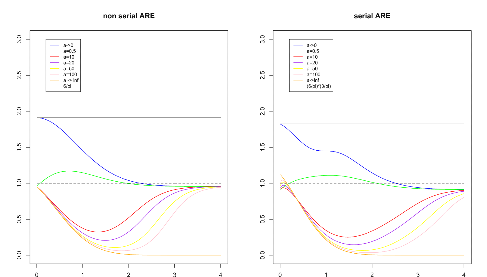
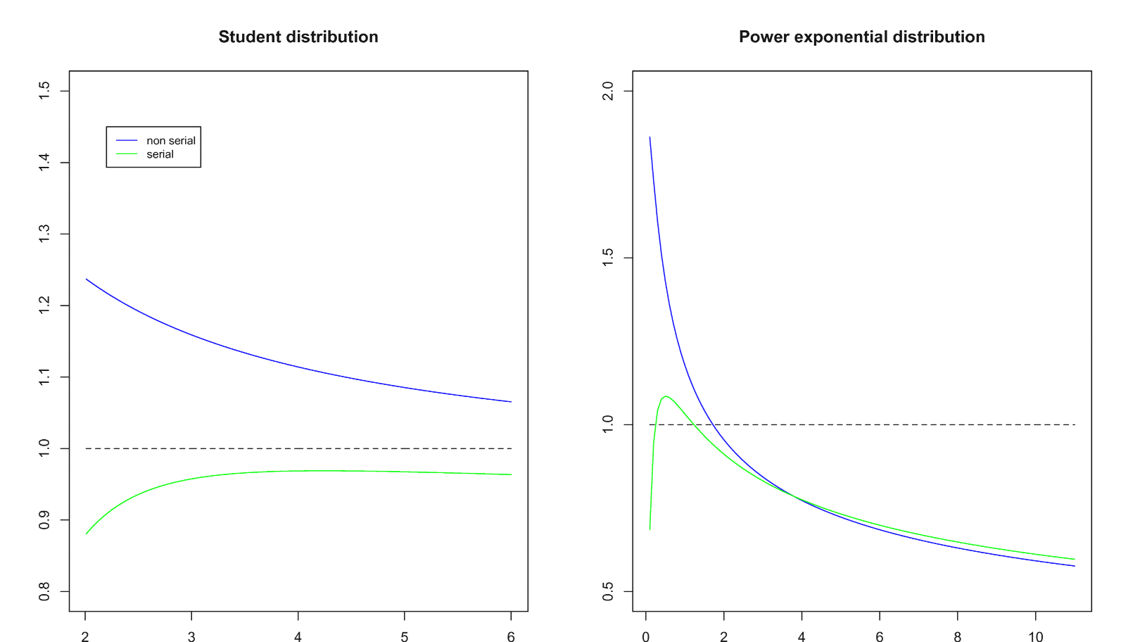
All tables seem to confirm the same findings : both the serial and the non-serial AREs are monotone in the size of the tails, with the non-serial AREf attaining its maximal value () under heavy-tailed densities, while the maximal value for the serial ARE lies somewhere around . Inspection of Table 1 reveals that, although the limit of as is monotone in the parameter , the ratio is not; from Table 3, the highest values of under the distribution (3.1) are attained for and .
Under Student densities , the nonserial AREf is decreasing with , taking value 1.41277 at the Cauchy (), value one about (a value of that is not shown in the figure; Wilcoxon is thus outperforming van der Waerden up to degrees of freedom, with van der Waerden taking over from on), and tending to the Gaussian value as ; the serial ARE is undefined for , increasing for small values of , from an infimum of 0.878736 (obtained as ) up to a maximum of 0.968852 (reached about ), then slowly decreasing to the Gaussian value 0.911891 as . Sperman-Wald-Wolfowitz and Kendall thus never outperform van der Waerden autocorrelations under Student densities.
Under the double exponential densities , the nonserial AREf is decreasing with , with a supremum of (the Hodges-Lehmann bound, obtained as ), and reaches value one about (similar local asymptotic performances of Wilcoxon and van der Waerden, thus, occur at power-exponentials with parameter ); the serial ARE is quite bad as , then rapidly increasing for small values of , with a maximum of 1.08552 about , then deteriorating again as ; for larger than 3, the serial and nonserial AREs roughly coincide.
Acknowledgments
This note originates in a research visit by the last two authors to the Department of Operations Research and Financial Engineering (ORFE) at Princeton University in the Fall of 2012; ORFE ’s support and hospitality is gratefully acknowledged. Marc Hallin’s research is supported by the Sonderforschungsbereich “Statistical modelling of nonlinear dynamic processes" (SFB 823) of the Deutsche Forschungsgemeinschaft, a Discovery Grant of the Australian Research Council, and the IAP research network grant P7/06 of the Belgian government (Belgian Science Policy). We gratefully acknowledge the pertinent comments by an anonymous referee on the original version of the manuscript, which lead to substantial improvements.
References
- [1] H. Chernoff and I. R. Savage (1958). Asymptotic normality and efficiency of certain nonparametric tests. Annals of Mathematical Statistics 29, 972–994.
- [2] J.L. Gastwirth (1970). On asymptotic relative efficiencies of a class of rank tests. Journal of the Royal Statistical Society Series B 32, 227–232.
- [3] T.S. Ferguson, C. Genest, and M. Hallin (2000). Kendall’s tau for serial dependence. The Canadian Journal of Statistics 28, 587–604.
- [4] J. Hájek and Z. Šidák (1967). Theory of Rank Tests, Academic Press, New York.
- [5] M. Hallin (1994). On the Pitman non-admissibility of correlogram-based methods. Journal of Time Series Analysis, 15, 607–611.
- [6] M. Hallin (2012). Asymptotic Relative Efficiency. In W. Piegorsch and A. El Shaarawi Eds, Encyclopedia of Environmetrics, 2nd edition, Wiley, 106-110.
- [7] M. Hallin and D. Paindaveine (2002). Optimal tests for multivariate location based on interdirections and pseudo-Mahalanobis ranks. Annals of Statistics 30, 1103-1133.
- [8] M. Hallin and D. Paindaveine (2002). Optimal procedures based on interdirections and pseudo-Mahalanobis ranks for testing multivariate elliptic white noise against ARMA dependence. Bernoulli 8, 787-815.
- [9] M. Hallin and D. Paindaveine (2004). Rank-based optimal tests of the adequacy of an elliptic VARMA model. Annals of Statistics 32, 2642–2678.
- [10] M. Hallin and D. Paindaveine (2005). Affine-invariant aligned rank tests for the multivariate general linear model with ARMA errors. Journal of Multivariate Analysis 93, 122-163.
- [11] M. Hallin and D. Paindaveine (2006). Semiparametrically efficient rank-based inference for shape: I Optimal rank-based tests for sphericity. Annals of Statistics 34, 2707–2756.
- [12] M. Hallin and D. Paindaveine (2008a). Chernoff-Savage and Hodges-Lehmann results for Wilks’ test of independence. In N. Balakrishnan, Edsel Pena and Mervyn J. Silvapulle, Eds, Beyond Parametrics in Interdisciplinary Research : Festschrift in Honor of Professor Pranab K. Sen. I.M.S. Lecture Notes-Monograph Series, 184–196.
- [13] M. Hallin and D. Paindaveine (2008b). Optimal rank-based tests for homogeneity of scatter. Annals of Statistics 36, 1261-1298.
- [14] M. Hallin and M.L. Puri (1988). Optimal rank-based procedures for time-series analysis: testing an model against other models. Annals of Statistics 16, 402-432.
- [15] M. Hallin and M.L. Puri (1992). Rank tests for time series analysis. In New Directions In Time Series Analysis (D. Brillinger, E. Parzen and M. Rosenblatt, eds), Springer-Verlag, New York, 111-154.
- [16] M. Hallin and M.L. Puri (1994). Aligned rank tests for linear models with autocorrelated error terms. Journal of Multivariate Analysis 50, 175-237.
- [17] M. Hallin, Y. Swan, T. Verdebout, and D. Veredas (2011). Rank-based testing in linear models with stable errors. Journal of Nonparametric Statistics 23, 305–320.
- [18] M. Hallin, Y. Swan, T. Verdebout, and D. Veredas (2013). One-step R-estimation in linear models with stable errors. Journal of Econometrics 172, 195–204.
- [19] M. Hallin and O. Tribel (2000). The efficiency of some nonparametric competitors to correlogram-based methods. In F.T. Bruss and L. Le Cam, Eds, Game Theory, Optimal Stopping, Probability, and Statistics, Papers in honor of T.S. Ferguson on the occasion of his 70th birthday, I.M.S. Lecture Notes-Monograph Series, 249-262.
- [20] J.L. Hodges and E.L. Lehmann (1956). The efficiency of some nonparametric competitors of the -test. Annals of Mathematical Statistics 2, 324–335.
- [21] J.L. Hodges and E.L. Lehmann (1961). Comparison of the normal scores and Wilcoxon tests. Proceedings of the Fourth Berkeley Symposium on Mathematical Statististics and Probability Vol. 1, 307–318.
- [22] H.L. Koul and A.K.Md.E. Saleh (1993). R-Estimation of the parameters of autoregressive AR models. The Annals of Statistics 21, 685–701.
- [23] H.L. Koul and A.K.Md.E. Saleh (1995). Autoregression quantiles and related rank-scores processes. . The Annals of Statistics 25, 670–689.
- [24] Y. Nikitin (1995). Asymptotic Efficiency of Nonparametric Tests. Cambridge University Press, Cambridge.
- [25] G.E. Noether (1955). On a theorem of Pitman. Annals of Mathematical Statistics 26, 64–68.
- [26] D. Paindaveine (2004). A unified and elementary proof of serial and nonserial, univariate and multivariate, Chernoff–Savage results. Statistical Methodology 1, 81–91.
- [27] D. Paindaveine (2006). A Chernoff–Savage result for shape: on the non-admissibility of pseudo-Gaussian methods. Journal of Multivariate Analysis 97, 2206–2220.
- [28] E.J.G. Pitman (1949). Notes on Nonparametric Statistical Inference. Columbia University, mimeographed.
- [29] M.L. Puri and P.K. Sen (1985). Nonparametric Methods in General Linear Models, J. Wiley, New York.
- [30] R.H. Randles and D.A. Wolfe (1979). Introduction to the theory of nonparametric statistics. John Wiley & Sons, New York.
- [31] R. Serfling (1980). Approximation Theorems of Mathematical Statistics. John Wiley & Sons, New York.
- [32] A.W. van der Vaart (1998). Asymptotic Statistics. Cambridge University Press, Cambridge.
- [33] A. Wald and J. Wolfowitz (1943). An exact test for randomness in the nonparametric case based on serial correlation. Annals of Mathematical Statistics 14, 378-388.
- [34] F. Wilcoxon (1945). Individual comparisons by ranking methods. Biometrics Bulletin 1, 80Ð83.