gbsn
Strangeness and charmness content of the nucleon from overlap fermions on -flavor domain-wall fermion configurations
Abstract
We present a calculation of the strangeness and charmness contents and of the nucleon from dynamical lattice QCD with flavors. The calculation is performed with overlap valence quarks on 2+1-flavor domain-wall fermion gauge configurations. The configurations are generated by the RBC collaboration on a lattice with sea-quark mass , , and inverse lattice spacing . Both actions have chiral symmetry which is essential in avoiding contamination due to the operator mixing with other flavors. The nucleon propagator and the quark loops are both computed with stochastic grid sources, while low-mode substitution and low-mode averaging methods are used respectively which substantially improve the signal-to-noise ratio. We obtain the strangeness matrix element , and the charmness content which is resolved from zero by 3 precision for the first time.
pacs
12.38.Gc, 14.20.Dh, 11.30.Hv, 14.65.DwI Introduction
The strangeness and charmness content of the nucleon are of fundamental importance to our understanding of the sea-quark contribution to nucleon structure. In particular, the sea-quark contribution to the scalar quark content is crucial to furthering our understanding of the pion-nucleon sigma term. In addition to their relevance to nucleon structure, the strangeness and charmness content of the nucleon have drawn recent interest due to their relevance in dark matter searches [1, 2, 3]. One popular candidate for dark matter is a weakly interacting massive particle (WIMP). The scalar (spin-independent) effective four-fermion interaction between the WIMP and the quarks, such as the neutralino-nucleon scattering in the context of the minimal supersymmetric standard model, is [1, 2]. Additionally, the scalar neutralino-nucleus coupling is found to be much larger than the axial-vector coupling [4]. In this case, the scalar contribution to the total -nucleus cross section is
| (1) |
where is the reduced -nucleus mass and
| (2) |
where , and
| (3) | |||||
| (4) |
are the contributions for the light ()and heavy () quarks respectively. From the trace anomaly for the nucleon mass
| (5) |
and the heavy-quark expansion [5], one can relate the glue condensate in the nucleon to the heavy-quark condensate. Equation (5) becomes
| (6) |
and Eq. (2) is written as
| (7) |
where . This expression is most often used in the analysis for dark matter searches [1, 2, 3]. Since the couplings and contain many terms that are proportional to the quark mass, e.g. through Higgs exchange, we see from Eqs. (2) and (7) that the total spin-independent neutralino-nucleus cross section is mainly proportional to and . Thus, it is important to determine them precisely.
At energy scales comparable to , perturbative calculations of and in the nucleon are prohibitively difficult due to the nonperturbative nature of QCD. However, these sea-quark matrix elements are accessible to lattice calculations. The first lattice calculations of were done with Wilson fermions on quenched lattices and with heavy dynamical Wilson fermion configurations [6, 7, 8]. Those calculations gave relatively large values for on the order of [7]. More recent calculations with Wilson-clover dynamical fermions also yield large values (– [9, 10, 11], whereas calculations with fermions incorporating chiral symmetry result in much smaller on the order of a few percent [12, 13, 14, 15, 16, 17, 18, 19].
The large value for found using Wilson-type fermions is due to the additive renormalization of the quark mass due to the lattice-spacing-dependent chiral symmetry breaking. As a consequence, there is mixing between the and operators and the operator [20] [12]. This leads to a subtraction term from which is proportional to the matrix element . Since the latter involves the valence contribution, the subtraction turns out to be large. For example, it is found that
| (8) |
is changed from to after the subtractions for the lattice with the nonperturbatively improved clover fermions [20]. Similarly, becomes after subtraction for the , lattice with Wilson-clover fermions [21]. An alternative way of evaluating the strangeness matrix element is to apply the Feynman-Hellman theorem and take the derivative with respect to and instead of the strange quark mass [22]. This approach avoids the additive mass part of the subtraction [12] and leads to a small [22].
To avoid the large systematic errors caused by explicit chiral symmetry breaking with Wilson-type fermions, we instead adopt overlap fermions with exact chiral symmetry on the lattice for the valence and the quark loop, for which the quark mass receives no additive renormalization.
In addition to having small discretization errors [23, 24], the overlap fermion that we use for the valence quarks in the nucleon can also be used for the light and charm quarks in the loop insertion with small error [25, 26]. This allows us to calculate both and .
For a heavy quark of flavor , it is shown [5] that, to leading order in the heavy quark expansion, the matrix element is related to the glue condensate in the nucleon,
| (9) |
If and quarks are all considered to be heavy and the light quark contributions are ignored, the combination of the trace anomaly and Eq. (9) predicts
| (10) |
It would be interesting to check this prediction by a direct lattice calculation, since the heavy quarks provide a significant contribution to the WIMP-on-nucleon cross section. In previous calculations, the charmness content of the nucleon has been obtained with the MILC HISQ configurations [16] with a 2 signal. In this work, we calculate the strangeness and charmness content of the nucleon in lattice QCD with overlap valence quarks on 2+1-flavor domain-wall fermion gauge configurations.
The calculation is done on a lattice with sea-quark mass , , and lattice spacing . We obtain the strangeness content which has more than 5 precision. Compared with previous lattice calculations either with disconnected insertion or via the Feynman-Hellman theorem [9, 10, 12, 13, 15, 16, 17, 18, 19, 21, 22], the present calculation has the smallest error. We also obtain the charmness content . This is the first time the charmness has been calculated with more than 3 precision.
Our paper is organized as follows. The overlap formulation is briefly summarized in Sec. II. The technical details for calculating the nucleon two-point functions and the quark loops are described in Sec. III and Sec. IV respectively. They are combined to calculate the disconnected three-point functions in Sec. V. Finally, the numerical results with chiral extrapolation are presented in Sec. VI and the conclusions are given in Sec. VII.
II Overlap Fermions
We adopt the overlap fermion formulation for the valence quarks in the nucleon correlation functions as well as for the quark loops. The inversion of overlap fermions using deflation of low eigenmodes and the construction of meson and nucleon two-point functions with low-mode substitution have been detailed previously [26]. Deflation with low eigenmodes and hypercubic smearing speed up the inversion by a factor of for the lattice that we use for this calculation and low-mode substitution (LMS) improves the errors of the meson and nucleon correlators by a factor of 3 – 4 [26]. The overlap quark propagators are calculated on gauge configurations with -flavors of dynamical domain-wall fermions (DWF). As we mentioned in the Introduction, we adopt both the overlap and DWF fermion formalisms since they preserve chiral symmetry via the Ginsparg-Wilson relation. Due to the high degree of chiral symmetry, the calculation of the quark content is free of the problems that plague the Wilson-type fermions as outlined in the above discussion. As an additional advantage, the discretization errors are small for the overlap fermion. This allows us to compute the charmness contribution to the nucleon in addition to the strangeness contribution.
The overlap operator [27] is defined as
| (11) |
where is the matrix sign function and is the usual Wilson fermion operator, except with a negative mass parameter in which . We set in our calculation, corresponding to . The massive overlap Dirac operator is defined as
| (12) | |||||
To accommodate the chiral transformation, it is usually convenient to use the chirally regulated field in lieu of in the interpolation field and the currents. This leads to an effective propagator
| (13) |
where is chiral, i.e. [28]. It is worthwhile to point out that this effective propagator has the same form as that in the continuum [25]. In other words, the inverse of the propagator is a chirally invariant massless Dirac operator plus the quark mass term. As long as the error is small, this formulation is suitable for both light and heavy quarks.
We adopt the Zolotarev approximation to evaluate the matrix sign function. This entails two nested conjugate gradient loops to calculate the propagator of the overlap fermion. For each conjugate gradient loop, we use deflation with low eigenmodes to speed up the inversion. The details are given in Ref. [26]. Due to the normality of , i.e. and the Ginsparg-Wilson relation , the eigenvalues of are on a unit circle with the center at unity. The real and chiral modes are at 0 and 2. Others on the circle are paired with conjugate eigenvalues. In other words, if is an eigenvector
| (14) |
then its conjugate partner is also an eigenvector with eigenvalue ,
| (15) |
To compute the quark propagator, we first find a few hundred pairs of the lowest eigenvectors of the massless overlap operator in addition to the zero modes. Once we have obtained these lowest eigenvectors, we can solve the high-mode part of the quark propagator by projecting out the low modes from the source
| (16) |
where is the source vector and the factor takes care of the zero modes which are either left-handed or right-handed.
In contrast, the low-mode part of the effective quark propagator can be constructed with eigenvectors directly,
| (17) |
For a given source , the total effective quark propagator is
| (18) |
However, we should point out that since is constructed from the eigenmodes rather than by inverting a source vector, we can compute the any-to-any propagator for any source and sink location with little additional computation. We shall use this fact to carry out the low-mode substitution to replace in Eq. (18) with for a source with given grid points which greatly improves the nucleon correlator. This will be explained in more detail in the next section.
III The Nucleon Two-Point Correlation Function
Various attempts have been made to improve the statistics of hadronic two-point correlation functions such as using a smeared source, a volume source with fixed gauge, and all-to-all propagators. The computation of all-to-all propagators usually involves noise sources on different sites. However, the quark propagator from one site can be contaminated by those from neighboring sites. For example, when constructing the nucleon correlation function, the three quark propagators may be from the same source site or from different source sites. The latter case is not gauge-invariant and will introduce noise after averaging over a finite number of configurations. Fig. 1 shows the gauge-invariant and the noninvariant parts of the correlation function.

The signal-to-noise issue has been examined [26] for the connected hadron correlators from the noise source on a time slice and it was found that the noise wall source was worse than the point source for all mesons except the pion. It is worse still for the nucleon. In this case, the signal-to-noise ratio is
| (19) |
where is the number of noises and is the three-volume of the time slice. In addition to the usual exponential suppression in time, there is a prefactor which reduces the signal-to-noise ratio further by a factor of . The situation can be ameliorated by reducing the noise contamination from neighboring sites with less source points. This introduces the idea of a noise grid source with support on some uniformly spaced grid points on a time slice, but this does not fundamentally alter the conclusion that, given the same computer time, any noise source is worse than the point source for the meson and nucleon. These observations suggest a new algorithm for the grid noise with low-mode substitution (LMS) to reduce the variance from noise contamination while simultaneously addressing the low-mode correlation [26]. The idea is to replace the low-mode part of the quark propagator estimated from noise sources by the exact in Eq. (17) when all three quarks are in the low modes or when two quarks are in the low modes and the third is in the high modes – in constructing the baryon correlators to reduce the noise contributions shown in Fig. 1. It turns out that this LMS is quite successful. It reverses the above-mentioned trend that a noise source is worse than a point source and instead reduces the errors compared to the point source [26].
The grid noise is
| (20) |
where is a sparse grid of lattice sites on a time slice, and is the random phase on site with the property and . Tests on the lattice with a noise on 64 evenly spaced grid points on a time slice and with LMS reveal that for light quarks (pion masses at MeV) the errors of the meson and nucleon masses can be reduced by a factor of 3 to 4 as compared to the point source [26].
Since the nucleon has a physical size of – fm as deduced from its axial and electromagnetic form factors, a smeared source for the nucleon usually leads to a reduction of errors for the nucleon mass from the point source. In view of this, we introduce a smeared-grid source to increase the overlap with the nucleon ground-state wave function and diminish the contribution from the radially excited states and the collateral scattering states. We adopt the gauge-invariant spatial Gaussian smearing [29] on the grid source,
| (21) |
where is the smearing operator. By design, the smearing operator should produce a Gaussian distribution with a Klein-Gordon propagator. It is computed as an iteration of many small smearing steps,
| (22) |
where is the input width for a Gaussian distribution and is the number of smearing steps. The corresponding quark propagator with a smeared source is
| (23) | |||||

To check if the actual width from the smearing procedure is consistent with the input width parameter , we first define the actual smearing size by
| (24) |
where, for each spatial position , is the norm over spin and color of the smeared source vector which is created from a point source vector . Then we plot vs for different step sizes in Fig. 2. We see that for a given , there is a range of where the resultant smearing size has a nearly linear relation with . Beyond that range, flattens off as increases. As increases, the range for the near-linear relation expands. Even though we do not have evidence that the smeared source, when its is much smaller than the input , leads to ill physical effects, we think it is safe to keep the linear relationship. Consequently, we will use sufficient for a prescribed width so that and are in the linear range.

We choose the parameters and for this work which give a smearing size . The smeared distribution for a typical configuration is plotted in Fig. 3 which is indeed close to a Gaussian shape. This particular choice of and is aimed at increasing the overlap with the nucleon wave function while simultaneously minimizing contamination from different grid sites.
In addition to the smearing source, we also placed two sources on the time slices and and calculated the inversion simultaneously. As we shall see later in the calculation of the nucleon mass and quark scalar matrix elements, the time window for the fitting range is between to which is far from the two sources such that the contamination from the time backward propagating state from the second source at a distance of time slices away is negligible. This approach nearly doubles our statistics without computational overhead.
The local interpolating operator of the nucleon is taken to be [30]
| (25) |
where in the Pauli-Sakurai gamma-matrix convention. The color indices are denoted with latin letters and the Dirac indices are denoted with greek letters. The nucleon correlation function is constructed as
| (26) |
where the stands for the / quark propagator from the site to and the color indices from to . The average is taken over the different gauge configurations and noise sources. is defined as . The trace and the transpose operations only act on Dirac indices. When the masses of the and quarks are set to be equal, and are the same propagator. The correlation function is a linear functional of the three functions , and .
From Eq. (23), we obtain the quark propagator as a summation of the propagators from different grid sites with different phases:
| (27) |
where
| (28) |
The nucleon correlation function can be written as
| (29) | |||||
where denotes the correlator in a gauge configuration. is the correlator of a point or a smeared source at site for a gauge configuration. Thus, given a sufficient number of noise vectors and/or gauge configurations, this effectively increases the statistics of the correlator by the number of the grid points as compared to that of the point source.
Since we compute the quark propagator by splitting it into the low-mode and the high-mode pieces
| (30) | |||||
the nucleon correlation function can be split into contributions from the low modes and the high modes
| (31) | |||||
where both and are noise-estimated propagators. We denote the latter explicitly because we will modify it below to improve the signal-to-noise ratio.
We first note that the last four terms with a summation over different noises, i.e. terms with and are pure noise. They can be dropped without changing the expectation value of the noise estimate. For the purely high-mode contribution, as well as the mixed terms containing two and a single , one needs to compute them with the noise technique. However, for the correlators either involving three or with two and one , one can implement the LMS [26] to improve the signal. For the case where all the propagators are purely from the low modes, we substitute the noise-estimated one [the second term on the right side of Eq. (31)] with the exact expression without noise, i.e. which is the sum of the low-mode contribution to point-source correlators over the grid points. For those terms containing only one and two , we replace the noise-estimated correlator [the sixth through eighth terms on the right side of Eq. (31)] with the one where the sources of the two are placed at the same grid site and multiplied with . This ties them with , which contains a , to form the less noisy multiple-point nucleon correlator over the grid points. (See the upper part of Fig. 1.) Since we replaced two noise-estimated with one noise-estimated , this should yield a gain in the signal-to-noise ratio by , where is the number of grid points.
Therefore, the nucleon correlator with LMS is
| (32) | |||||
We should point out that this is different from low-mode averaging [31, 32] in that the noise-estimated low-mode propagators in LMS are substituted with the exact ones whenever possible and matched with the high-mode propagators at the grid points, whereas low-mode averaging would replace the noise-estimated low-mode part with the average over all space-time points.
Ideally, we would compute a separate set of quark propagators from each source point on the grid source, eliminating those gauge-dependent contributions to the two-point function (which contribute only noise) where the propagators come from different source points while still gaining the benefits of the extra sources. However, this is prohibitively expensive, as it requires additional inversions. As mentioned previously, the grid source is chosen in order to achieve some of the benefits of using multiple spatial sources while requiring no additional inversions, but noise is introduced by those contributions which mix the various source locations. However, the purely low-mode part requires no inversions to calculate, so it can be computed exactly without noise from these spurious contributions. Since this low-mode contribution dominates the correlation function at large time separation, the use of the low modes to compute it exactly allows for a substantial reduction in the error of the nucleon mass.
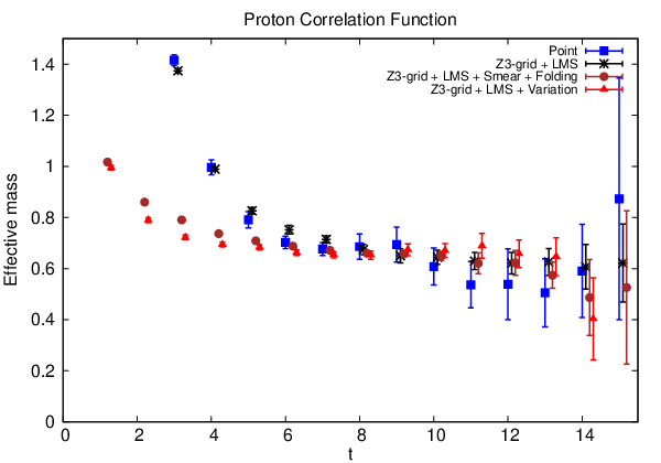
In Fig. 4, we plot the effective masses of the nucleon correlation functions from the point source, the noise-grid source, the noise-grid source with smearing and folding of the two correlators from sources on two time slices at and , and the variation calculation with the point and the noise-grid source. The fitted masses are tabulated in Table 1. They are calculated on the ensemble of 50 flavor DWF configurations on the lattice with . The overlap propagator is computed with the valence quark mass at close to the light sea mass which corresponds to MeV.
| Point | -grid | -grid + LMS | -grid + LMS | |
| + LMS | + Smear + Folding | + Variation | ||
| Nucleon mass (GeV) | 1.13(14) | 1.08(5) | 1.14(2) | 1.12(1) |
We see the fitted nucleon mass for the point source has a error. The noise grid source with LMS reduces the error by a factor of down to . Replacing the point grid with a smeared grid and putting the sources on two time slices reduces the error further to . Finally, a variational calculation with a second nucleon interpolation field and smeared grid sources gives an error of . For this, the second nucleon interpolation field we use is and each quark in the interpolation field can be a point-grid or a smeared-grid source. The combination of point-grid and smeared-grid sources gives eight operators. Of these eight, we need to consider the symmetric combination between the two quarks so that they are spatially symmetric. This reduces the choice to six. We calculate all of the six combinations for each of the two interpolation fields (which differ in their Dirac structure) and during the analysis choose four of the twelve which have a good result for the ground state and a decent result for the lowest excited state. The operators of the variational calculation are obtained by choosing or and choosing all three quarks smeared or just one quark smeared.
It is worth emphasizing that replacing the point source by a point-grid source with LMS, with no further improvements, reduces the error by a factor of , improving the statistics by a factor of 8 with no added expense. For comparison, we note a recent study of the all-mode-averaging (AMA) method [33] on the same lattices which found that to achieve the same error on the nucleon mass with AMA on 32 smeared sources would cost 1/4 of the computer time of a single smeared source without AMA. This implies that AMA, given the same resources, would improve the statistics by a factor of 4.
The variational approach using two different interpolating fields combined with a mixed point/smeared source does reduce the variance, but not enough to justify the increased computational cost required for the additional point-source inversion. Overall, we find that the use of smeared noise-grid sources on two time slices is the most efficient approach; this reduces the error of the nucleon mass by a factor of 7 compared to that of the point source while adding only the slight overhead of LMS to the computational cost.
IV Quark Loops
The quark loop with zero momentum on a time slice is defined as where the trace is over color and spin and is a matrix. It is computed for the quark propagator which begins and ends at the same site (or more generally a neighboring site if a point-split current or smearing function is involved). It is needed for meson correlators with the quark-antiquark annihilation channels and the disconnected insertions in nucleon form-factor calculations. Since the quark-loop calculation involves the sum of quark propagators originating from all lattice sites on a time slice, it is not practical to calculate it with the usual point-source inversion. Instead, stochastic estimation is usually used for such calculations. Taking the noise source in Eq. (20) where the grid includes all lattice points, the loop at the position for each gauge configuration is then estimated as
| (33) | |||||
where the average is taken over the noise. When the noise source is diluted in color and Dirac indices, the loop is a matrix in color-spin space. For a finite number of noises, there is noise contribution from different sites which is not a gauge-invariant quantity and is suppressed by gauge averaging in addition to noise averaging. It has been shown that noise is optimal since it gives the minimum variance [34, 35]. Here we shall use the noise which, in addition to calculating loops, can be applied to the evaluation of quark annihilation involving two quarks and two antiquarks in the interpolation operators, such as in meson-meson scattering calculations.
In the nucleon three-point function involving the loops in the disconnected insertion (DI), the quark loop including the external current needs to be Fourier transformed to give a definite momentum transfer. Because of the translational invariance after gauge averaging, one does not need to put the noise on all spatial points at a given time slice. Instead, one could select an evenly spaced grid separated by sites in each of the spatial directions. In this case, the Fourier transformation of on a lattice with periodic boundary conditions can project to a low-momentum in the direction via the relation . Besides the definite momentum , it involves a mixture of the next higher momentum being , where is the spatial lattice dimension and is the unit of lattice momentum, i.e. . Other higher momenta can also be mixed in, but we will not discuss them here. In the nucleon DI calculation, the source and sink momenta of the nucleon propagator can have a definite momentum (the grid source for the nucleon propagator with will have a zero-momentum source mixed with ). As long as these mixed momenta are taken into account in selecting the desired momentum transfer, the mixed loop will be suppressed due to momentum conservation. Should it happen that the contribution from the mixed high-momentum loop with does not vanish due to the finite noise and gauge configurations, it will involve the intermediate state with energy . Its contribution is exponentially suppressed with a factor where . Since and thus , the suppression factor can be substantial for the range of where the signal of the DI calculation is to be obtained. For the present work, the scalar content is a forward matrix element which requires . This makes it easier to consider the possible contamination.
In our present calculation of the scalar matrix elements on the lattice, we shall use the grid with for the high modes with odd-even dilution as well as dilution in time. This entails the calculation of four noise propagators (two for odd-even and two for time dilution). We show in Fig. 5 a cartoon of the even-odd dilution and the time dilution. The nearest neighbor which can give rise to noise contribution is at a Euclidean distance of which is reasonably far; as such, we do not do the unbiased subtraction as has been done previously for noises which have support on all lattice points [36, 7], where the nearest neighbor is a single lattice site away. Should there be noise contribution from the higher mixed momentum despite suppression due to momentum conservation as discussed above, it will be further suppressed by . With and , is 1.04. As a result, the suppression factor for where the strangeness matrix element will be extracted is less than which renders this noise contribution negligible.

To further improve the loop calculation, we use low-mode averaging (LMA) for the low-mode contribution by summing over the spatial volume on a time slice, while the high-mode contribution is calculated on the grid as described above.
| (34) |
where is scaled from the sum of the grid points to that of the full space volume to match with from LMA.

It is interesting to find out the individual contributions to the quark loops from the low modes and the high modes. To this end, we measure the following quantity to gauge the magnitude of the low-mode contribution relative to the sum of those of the low modes and the high modes,
| (35) |
The norms of the low- and the high-mode parts of the loops are used to avoid the singular situation when the full loop is near zero, especially for the vector and axial-vector channels, where the vacuum expectation values of the loops are zero. The ratio is taken before averaging over the time slices so as to be more relevant to the DI calculation where the loop is to be correlated with the nucleon propagator in a limited time range. We used five configurations in this study.

The relative magnitudes of the low modes, defined as in Eq. (35), in terms of the accumulated pairs of low eigenmodes in addition to the zero modes are shown in Fig. 6 for different currents. This is for the case of a quark mass which corresponds to a pion mass of MeV. We see that of the pseudoscalar loop is dominated by a few lowest eigenmodes, and all the higher modes contribute only a few percent. This is not surprising, since the space-time integral of the pseudoscalar density times the quark mass is just the topological charge of the configuration which is totally determined by the zero modes. For the scalar loop, both the and are positive on all time slices and for all configurations. Therefore, the relative magnitude is the relative low-mode contribution. In this case, of the scalar loop is contributed by the lowest 50 pairs of eigenmodes. Even at this low quark mass, most of the contribution comes from the high modes. In the vector and axial-vector channels, the relative low-mode magnitude is small with a large variance.
To study the quark-mass dependence, we show in Fig. 7 with 200 pairs of the lowest eigenmodes plus zero modes as a function of the quark mass. The relative magnitude of the low modes in the pseudoscalar channel dominates in the light quark region and decreases with quark mass. The for the scalar, vector, and axial loops decrease with quark mass faster than that of the pseudoscalar loop and become very small for MeV. This hints that for the charmness in the nucleon, the high modes may play a substantial role.
V Disconnected Insertion of The Three-Point Correlation Function
In order to extract the strangeness and charmness contributions to the nucleon given in Eq. (3), we compute the ratio of the disconnected three-point function to the two-point function, defined as
| (36) |
The matrix element for the quark content in the nucleon can be extracted from this ratio,
| (37) | |||||
For the disconnected insertion, one can write the above ratio in terms of the nucleon propagator and the quark loop as in Sec. IV,
| (38) |
This approach is illustrated in Fig. 8.
We show in Fig. 9 as a function of from to for the case where the quark mass in the loop is , which corresponds to the strange quark mass, and the quark mass in the nucleon propagator is , which corresponds to MeV. This calculation is done on 176 configurations. One can see that the error bars are quite large, and it appears to be difficult to determine a plateau region from which to extract the matrix element.


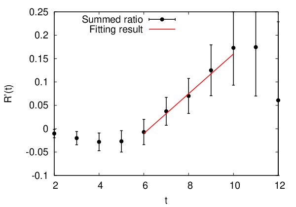
One can improve the statistics by using the summed ratio method [37]. As illustrated in Fig. 10, is summed over between and inclusive
| (39) |
Previous calculations of the quark momentum fraction in the DI [38], have studied various choices for the domain of . They found that choosing between and inclusive produced less noise than other choices. For this reason, we have chosen to adopt the same domain in our calculations.
The ratio method is a means to incorporate information from multiple values of and , thus reducing the statistical error, without needing to explicitly consider the points at which might suffer from excited-state pollution because they are too close to and . The method relies on the fact that when the value of is summed from source to sink, the contribution from these contaminated points near the end does not depend on the distance from source to sink so long as that distance is large enough. When the propagator length is increased, the additional contribution to the sum comes from a single point in the center, within the plateau region. Thus, by examining how much the summed ratio increases when the propagator length is increased, we can get an estimate for the plateau value of that incorporates information from multiple values of and .
It was shown [37, 38] that the ratio has a linear behavior in a region where is large enough to have a plateau in and thus
| (40) |
We fit the value of the summed ratio to constant-plus-linear over the range in which is large enough for to have a plateau; the slope in is thus a measurement of the plateau value of , i.e. the matrix element, from which the quark content is determined using Eq. (37). We should mention that the excited-state contamination in the sum method is found to be [38, 39] where is the energy gap between the nucleon ground state and the lowest excited state and is the sink time of the nucleon propagator (we have taken the source time at ). On the other hand, the contamination of the excited state in the plateau method is where is the time when the plateau appears and is the fixed sink time of the nucleon propagator. Since in practice and , the excited-state contamination is less than that of the plateau method and this has been demonstrated in the calculation of the isovector [39].


VI Numerical Results
This work is carried out using valence overlap fermions on 176 configurations with flavors of sea domain-wall fermions. The lattice size is with the inverse lattice spacing GeV. The / quark mass in the DWF sea is which corresponds to a pion mass of MeV. The sea strange-quark mass is . This pion mass is matched for the overlap fermion with a valence / quark mass of 0.016. With the help of the multimass algorithm [40], we compute a set of 26 quark masses for the nucleon and 10 for the loops with an overhead of about 8% [41] of the cost of inverting the lowest quark mass. The summed ratio of the strangeness is shown in Fig. 11 for and .
The nucleon propagator in the DI of the three-point function is calculated with a smeared grid source at and . The time-forward propagator with positive-parity projection and the time-backward propagator with negative-parity projection are averaged. We see that a linear slope develops after where the nucleon starts to emerge in the nucleon correlator and it is in the middle of the plateau from Fig. 9.
To see the contributions to and the respective slopes from the low modes and the high modes in the loop, we plot them separately in Fig. 11. It is interesting to observe that practically all the contributions to are coming from the low modes despite the fact that the low modes saturate only of the strange quark loop. The high-mode contribution is quite small. Since the low-mode contribution is exact, it only has variance from the gauge ensemble. The variance of the high-mode contribution comes from both the noise and gauge ensembles. Since its contribution is small, there is no need to improve this part of the estimate with more noise vectors.
The renormalized strangeness content reads
| (41) |
where the nonperturbative renormalization constant (stat) has been calculated in the regularization-independent momentum-subtraction renormalization scheme [42] with input of from the chiral Ward identity. It is plotted in Fig. 12 as a function of the valence quark mass. The results are obtained from fitting the range from to 14 in each quark-mass case. The lowest quark mass gives MeV.


To obtain a value at the physical point we must perform a chiral extrapolation. The mixed-action formula can be derived from the partially quenched expression in Ref. [43], using the simple conversion of partially quenched to mixed-action formulas described in Refs. [44, 45]. The next-to-leading-order mixed-action extrapolation formula is [46]
| (42) | |||||
where are the leading-order contributions to the strange matrix element in the chiral limit and the nonanalytic chiral loop function is [47]
| (43) |
where is the mass difference of the baryon and the nucleon.
In the case without an explicit delta degree of freedom, Eq. (42) can be simplified to
| (44) |
The only mixed action low-energy constant [44] between the valence overlap fermion and sea domain-wall fermions is found to be small [48] — it shifts the pion mass at MeV by a mere 16 MeV. We can safely neglect the mixed-action effects since they are quite small compared to the statistical error.
Combining Eq. (40) and Eq. (44), we obtain a global fit using different time slices and quark masses. The fitting model for strangeness reads
| (45) |
where and are the physical quark masses corresponding to the correct and masses, and is a set of constants.
After the chiral extrapolation in the valence quark mass and the interpolation in the loop quark mass, we get the renormalized strangeness matrix element and MeV with a fitting range from to 14 and . We also calculate the nucleon mass and extrapolate it to the chiral limit with as shown in Fig. 13 and we obtain GeV at the physical pion mass. Using this number, we obtain . We plot the recent results of in Fig. 14 from calculations with dynamical fermions with and (the ETM collaboration’s calculation is with ). We see that our result has a small statistical error and its relative error is comparable to those of Refs. [13, 15, 16].


Similarly, we can compute the charmness content using the same method. The summed ratio of the charmness is shown in Fig. 15 and the low/high separation is given in Fig. 15. We see that the low-mode part still plays an important role, but in contrast to the strangeness case, the high-mode contribution is no longer small.


The chiral extrapolation is shown in Fig. 16. We take which corresponds to the physical charm mass in the global analysis of the charmonium spectrum with three sea masses and two lattice spacings [49]. We find the renormalized charmness content and after the chiral extrapolation and charm-quark-mass interpolation. This number is consistent with the result from the MILC collaboration at [16], but with a smaller relative error at 33%. It is interesting to note that at MeV is larger than MeV and agrees with the prediction of 70 MeV in Eq. (10) from the heavy-quark expansion [5].
By varying the quark mass in the loop with a fixed light quark mass in the nucleon, we can check the quark-mass dependence of and . Figures 17 and 18 display the quark-mass dependence of and respectively as a function of the quark mass. We see that the matrix element seems to go down as at reasonably large and appears to be flat beyond MeV. This behavior will be checked with higher precision on the lattice with GeV which can accommodate heavier quark masses than on the present lattice.


VII Conclusion
In this work, we have computed both the strangeness and the charmness content of the nucleon with overlap valence fermions on -flavor dynamical DWF configurations on the lattice with GeV and a sea pion mass of 331 MeV. We have employed a smeared noise-grid source with low-mode substitution to calculate the nucleon two-point functions, which reduces the error on the nucleon mass by a factor of 7 compared to the calculation with a point source. For the loop part of the three-point disconnected insertion calculation, we used low-mode averaging to compute the low-mode part exactly and used the noise on a grid to estimate the high-mode part. It turns out that the high-mode part contributes negligibly to the strangeness content. With the highly improved nucleon propagators and the quark loops, we extrapolated to the physical pion mass and obtained the precise value with a better than 5 signal. The statistical error is quite small compared to those of other lattice calculations. The renormalized matrix element is and the strange-quark sigma term is MeV. Similarly, we obtain with a 3 signal which is the first time such a result has been obtained for the charm beyond a precision of two sigma. The renormalized matrix element is and the charm-quark sigma term is MeV which is consistent with the prediction based on the heavy quark expansion [5, 50].
Even though our present work has a high precision, a more meaningful comparison would be with the number of inversions one has to do in order to achieve the same precision. To this end, we shall compare our results with the calculations by Engelhardt [15] and JLQCD [18]. They used the direct DI calculation with DWF and overlap which should have an inversion time comparable to the overlap fermion we use. In our case, we used 176 configurations and 48 noise vectors to calculate the high-mode part of the quark loop. In the case of Engelhardt [15], configurations were used each with 1200 noise vectors, giving a relative error of 24% at sink time , comparable to our result. However, this approach requires times as many inversions as ours. As for the JLQCD calculation [18], 288 noise vectors were used on 50 configurations and the error is 2.54 times larger than ours. Thus, to reach the same error as ours, it would take this approach times as many inversions. We attribute the efficiency of our approach to the improvement of both the nucleon propagator and the quark loop.
In the present work we have considered the statistical error only. We will continue this work on the dislocation-suppressing determinant ratio lattices with GeV and and 250 MeV, as well as the finer lattices with GeV and MeV, in order to extrapolate to the continuum limit and the physical sea pion mass in order to address the systematic errors.
ACKNOWLEDGMENTS
We thank RBC and UKQCD for sharing the DWF gauge configurations that we used in the present work. We thank Stefan Meinel for his fitting code. We also thank Andre Walker-Loud for showing us the mixed-action partially quenched chiral perturbation expression in Eq. (44). K.F. L. wishes to thank the Nuclear Theory Group at Lawrence Berkeley Lab. for their hospitality where part of the manuscript was written up. This work is partially supported by DOE grants DE-FG05-84ER40154 and DE-FG02-00ER41132. A. A. is partially supported by NSF CAREER grant PHY-1151648. T. D. is partially supported in part by MEXT Grant-in-Aid for Young Scientists (B) (24740146). Z. L. is partially supported by NSFC under the Project 11105153.
References
- [1] T. Falk, A. Ferstl, and K. A. Olive, Phys.Rev. D 59, 055009 (1999).
- [2] J. R. Ellis, K. A. Olive, and C. Savage, Phys.Rev. D 77, 065026 (2008).
- [3] J. Giedt, A. W. Thomas, and R. D. Young, Phys.Rev.Lett. 103, 201802 (2009).
- [4] G. Jungman, M. Kamionkowski, and K. Griest, Physics Reports 267, 195 (1996).
- [5] M. A. Shifman, A. Vainshtein, and V. I. Zakharov, Phys.Lett. B 78, 443 (1978).
- [6] M. Fukugita, Y. Kuramashi, M. Okawa, and A. Ukawa, Phys.Rev. D 51, 5319 (1995).
- [7] S. Dong, J. Lagae, and K. Liu, Phys.Rev. D 54, 5496 (1996).
- [8] TXL Collaboration, S. Gusken, P. Ueberholz, J. Viehoff, N. Eicker, P. Lacock, et al., Phys.Rev. D 59, 054504 (1999).
- [9] S. Durr, Z. Fodor, T. Hemmert, C. Hoelbling, J. Frison, et al., Phys.Rev. D 85, 014509 (2012).
- [10] QCDSF-UKQCD Collaborations, R. Horsley, Y. Nakamura, H. Perlt, D. Pleiter, P. Rakow, et al., Phys.Rev. D 85, 034506 (2012).
- [11] R. Babich, R. C. Brower, M. A. Clark, G. T. Fleming, J. C. Osborn, et al., Phys.Rev. D 85, 054510 (2012).
- [12] JLQCD collaboration, K. Takeda, S. Aoki, S. Hashimoto, T. Kaneko, J. Noaki, et al., Phys.Rev. D83, 114506 (2011), 1011.1964.
- [13] MILC Collaboration, D. Toussaint and W. Freeman, Phys.Rev.Lett. 103, 122002 (2009).
- [14] M. Engelhardt, Proc. Sci. LATTICE, 137 (2010).
- [15] M. Engelhardt, Phys.Rev. D 86, 114510 (2012).
- [16] MILC Collaboration, W. Freeman and D. Toussaint, arXiv:1204.3866.
- [17] ETM Collaboration, S. Dinter, V. Drach, R. Frezzotti, G. Herdoiza, K. Jansen, et al., J. High Energy Phys. 08, 037 (2012).
- [18] JLQCD Collaboration, H. Ohki, K. Takeda, S. Aoki, S. Hashimoto, T. Kaneko, et al., Phys. Rev. D 87, 034509 (2013).
- [19] P. Junnarkar and A. Walker-Loud, arXiv:1301.1114.
- [20] UKQCD Collaboration, C. Michael, C. McNeile, and D. Hepburn, Nucl.Phys.Proc.Suppl. 106, 293 (2002).
- [21] QCDSF Collaboration, G. S. Bali, S. Collins, M. Gockeler, R. Horsley, Y. Nakamura, et al., Phys.Rev. D 85, 054502 (2012).
- [22] R. Young and A. Thomas, Phys.Rev. D 81, 014503 (2010).
- [23] S. Dong, F. Lee, K. Liu, and J. Zhang, Phys.Rev.Lett. 85, 5051 (2000).
- [24] T. Draper, N. Mathur, J. Zhang, A. Alexandru, Y. Chen, et al., Proc. Sci. LATTICE, 120 (2005).
- [25] K.-F. Liu and S.-J. Dong, Int.J.Mod.Phys. A 20, 7241 (2005).
- [26] xQCD Collaboration, A. Li, A. Alexandru, Y. Chen, T. Doi, S. Dong, et al., Phys.Rev. D 82, 114501 (2010).
- [27] H. Neuberger, Phys.Lett. B 417, 141 (1998).
- [28] T.-W. Chiu and S. V. Zenkin, Phys.Rev. D59, 074501 (1999).
- [29] C. Alexandrou, S. Gusken, F. Jegerlehner, K. Schilling, and R. Sommer, Nucl.Phys. B414, 815 (1994).
- [30] W. Wilcox, T. Draper, and K.-F. Liu, Phys.Rev. D 46, 1109 (1992).
- [31] H. Neff, N. Eicker, T. Lippert, J. W. Negele, and K. Schilling, Phys.Rev. D 64, 114509 (2001).
- [32] L. Venkataraman and G. Kilcup, Nucl.Phys.Proc.Suppl. 63, 826 (1998).
- [33] T. Blum, T. Izubuchi, and E. Shintani, Proc. Sci. LATTICE, 262 (2012).
- [34] S. Bernardson, P. McCarty, and C. Thron, Comput.Phys.Commun. 78, 256 (1993).
- [35] S.-J. Dong and K.-F. Liu, Phys.Lett. B 328, 130 (1994).
- [36] C. Thron, S. Dong, K. Liu, and H. Ying, Phys.Rev. D 57, 1642 (1998).
- [37] L. Maiani, G. Martinelli, M. Paciello, and B. Taglienti, Nucl.Phys. B293, 420 (1987).
- [38] M. Deka, T. Streuer, T. Doi, S. Dong, T. Draper, et al., Phys.Rev. D 79, 094502 (2009).
- [39] S. Capitani, M. Della Morte, G. von Hippel, B. Jager, A. Juttner, et al., Phys.Rev. D 86, 074502 (2012).
- [40] B. Jegerlehner, arXiv:hep-lat/9612014.
- [41] H.-P. Ying, S.-J. Dong, and K.-F. Liu, Nucl.Phys.Proc.Suppl. 53, 993 (1997).
- [42] xQCD Collaboration, Z. Liu et al., (to be published).
- [43] J.-W. Chen and M. J. Savage, Phys.Rev. D 66, 074509 (2002).
- [44] J.-W. Chen, D. O’Connell, and A. Walker-Loud, Phys.Rev. D 75, 054501 (2007).
- [45] J.-W. Chen, D. O’Connell, and A. Walker-Loud, J. High Energy Phys. 04, 090 (2009).
- [46] A. Walker-Loud, (private communication).
- [47] B. C. Tiburzi and A. Walker-Loud, Nucl.Phys. A764, 274 (2006).
- [48] M. Lujan, A. Alexandru, Y. Chen, T. Draper, W. Freeman, et al., Phys.Rev. D 86, 014501 (2012).
- [49] xQCD Collaboration, Y. Yang et al., (to be published).
- [50] A. Kryjevski, Phys.Rev. D 70, 094028 (2004).