Long-time asymptotics for the porous medium equation: The spectrum of the linearized operator Note: The author acknowledges support through NSERC grant 217006-08.

In order to investigate the asymptotic behavior of solutions to the porous medium equation, it is convenient to rescale variables in such a way that the Barenblatt solution becomes a stationary solution, that means $|x|\sim t^{\alpha}$ in view of (2). One convenient choice of new variables is

with

to the effect of

We remark that the logarithmic rescaling of the time variable, $\hat{t}=\alpha\ln t$, guarantees the parabolic structure of the equation. In fact, with its new variables, equation (1) turns into the nonlinear Fokker–Planck equation

sometimes also called the confined porous medium equation. Moreover, with that particular choice of $\beta$, the rescaled, time-independent Barenblatt solution $\hat{\rho}_{*}$ concentrates on a ball of radius one around the origin,

This normalization will simplify the notation in the subsequent sections. In the sequel, we will often refer to $\hat{\rho}_{*}$ as the Barenblatt profile.

The advantage of working with (3) instead of (1) relies on the fact that the above rescaling comes along with a change of perspective: the Barenblatt solution now becomes a fixed point of the equation. In fact, as we will see below, for fixed total mass $\hat{M}$, it is both the unique stationary solution of (3) and the ground state of the physical entropy

In this regard, the porous medium equation (1) shows a substantially different behavior than the confined porous medium equation (3): There is no stationary solution of (1) under the mass constraint $\|\rho\|_{L^{1}}=M$ for any $M>0$. In other words, solutions to the porous medium equation do not relax in finite time and the ground state can be attained only asymptotically in the long-time limit.

Somehow related to this feature is the fact that, opposed to the original equation (1), the confined porous medium equation (3) is no longer invariant under spatial translations. More precisely, in the new variables the origin is the unique attraction point in $\mathbbm{R}^{N}$ around which the mass asymptotically concentrates, driven by the convection term $-\hat{\nabla}\cdot(\hat{x}\hat{\rho})$. Due to this loss of translation invariance it is therefore not surprising that those initial data $\hat{\rho}_{0}$ that differ from the ground state $\hat{\rho}_{*}$ only by a shift, $\hat{\rho}_{0}(\hat{x})=\hat{\rho}_{*}(\hat{x}-\hat{x}_{0})$ for some $\hat{x}_{0}\in\mathbbm{R}^{N}$, will play a distinguished role in the discussion of our result on refined asymptotics of (3): Spatial translations correspond to the smallest eigenvalue of the linearized operator and generate thus those solutions that saturate the optimal rate of convergence.

The above rescaling, however, also has a small drawback: It is singular at time zero. To compare “initial data”, one would better consider the moment $t=1$. More precisely, up to spatial dilations both in the $x$ and $\rho$ variables, the initial datum $\hat{\rho}(\hat{t}=0,\,\cdot\,)$ corresponds to the original solution at time one $\rho(t=1,\,\cdot\,)$. Because of our interest in the long-time dynamics, this skew correspondence, however, has no influence neither on the subsequent analysis nor on the interpretation of our result.

It remains to discuss the stationarity of $\hat{\rho}_{*}$ for the nonlinear Fokker–Planck equation (3) and its minimality for the entropy (5). Calculating the energy dissipation along trajectories of the flow (3),

we see that the dissipation rate is zero if and only if $\frac{1}{2}|\hat{x}|^{2}+\frac{m}{m-1}\hat{\rho}^{m-1}$ is constant, that is, if and only if $\hat{\rho}$ is of the form (4), provided that $\hat{\rho}$ and $\hat{\rho}_{*}$ have the same total mass. This implies that $\hat{\rho}_{*}$ is the unique stationary solution of (3). To deduce the minimality of $\hat{\rho}_{*}$ for the entropy $\hat{E}$, we additionally observe that the entropy is strictly convex on the convex configuration space of nonnegative densities with fixed total mass $\hat{M}$ and admits thus a unique minimizer.

In his seminal paper [22], Otto introduced a new and physically meaningful gradient flow interpretation of the porous medium equation (1). This interpretation is based on the Lyapunov approach of Newman & Ralston in [20, 27]. In the abstract setting, a gradient flow is the dynamical system on a Riemannian manifold $(\mathcal{M},\mbox{\sl g})$ that describes the evolution as the steepest descent in an energy landscape, i.e.,

Here, the gradient $\gradient E$ of the energy $E$ is defined via Riesz’ representation theorem

where $\mbox{\rm diff}E$ denotes the differential of $E$ and $T_{\rho}\mathcal{M}$ is the tangent plane at the point $\rho\in\mathcal{M}$. A short formal computation shows that (6) can be equivalently stated as

In the following, we identify the gradient flow ingredients $\mathcal{M}$, g, and $E$ that constitute the porous medium equation using Otto’s approach. (In fact, different gradient flow interpretations were proposed for the porous medium equation. Otto’s gradient flow is natural in view of the thermodynamical background of the equation. Moreover, it also pertains to the confined evolution, whereas the traditional approaches do not.)

As solutions to (1) preserve non-negativity (in fact, solutions satisfy a comparison principle) and the total mass $M$, the manifold in the gradient flow interpretation of the porous medium equation has to be chosen as

Tangent fields $\delta\rho$ at $\rho\in\mathcal{M}$ must be mass-preserving and non-negative where $\rho=0$. For tangent fields satisfying $\spt(\delta\rho)\subset\spt(\rho)$, the metric tensor is defined by

where $\psi$ and $\delta\rho$ are related via the elliptic boundary value problem

Here, $\nu$ denotes the outer normal vector on $\partial\supp(\rho)$. The second condition has to be interpreted as an “asymptotic” boundary condition, see also (17) or Remark 1 below. Notice that $\nabla\psi$ may be non-zero on $\partial\supp(\rho)$, so that the boundary is “free” fo move. For all other tangent fields, we set $\mbox{\sl g}_{\rho}(\delta\rho,\delta\rho)=+\infty$. Actually, arguing even more formally, Otto set the elliptic problem (8) in the entire space $\mathbbm{R}^{N}$, cf. [22, eq. (8)]. However, in order to motivate our later analysis, here, we equip the equation with its natural boundary conditions. That is, assuming enough regularity of $\rho$ and $\delta\rho$, the distributional solution $\psi$ of $-\nabla\cdot\left(\rho\nabla\psi\right)=\delta\rho$ satisfies (8). Equivalently, we can characterize the metric tensor variationally:

cf. [23, eq. (2.9)], where the supremum is taken over all smooth functions $\varphi$ on $\mathbbm{R}^{N}$. Indeed, $\mbox{\sl g}_{\rho}(\delta\rho,\delta\rho)$ is finite if and only if $\spt(\delta\rho)\subset\spt(\rho)$, and then the optimal $\varphi$ in this formulation satisfies (8). When studying the gradient flow dynamics (7), it is enough to restrict the tangent plane to those tangent fields for which the metric tensor is finite. Hence, by identifying tangent fields $\delta\rho$ with the variables $\psi$ via (8), the tangent plane at $\rho$ can be written as the weighted Sobolev space

The energy functional in the gradient flow interpretation is given by the entropy

A short computation now shows the porous medium equation (1) is indeed the gradient flow for $(\mathcal{M},\mbox{\sl g})$ and $E$ defined as above, see [22, Sec. 1.3] for details.

As for the confined porous medium equation (3), we remark that $\hat{\rho}$ still evolves according to the gradient flow on the same Riemannian manifold as $\rho$, now with total mass $\hat{M}$ and denoted by $(\hat{\mathcal{M}},\hat{\mbox{\sl g}})$, but for the energy $\hat{E}$ defined in (5).

We finally address the induced geodesic distance on the Riemannian manifold $(\hat{\mathcal{M}},\hat{\mbox{\sl g}})$. Benamou & Brenier [5] discovered the relation between the Kantorovich mass transfer problem and continuum mechanics by identifying the geodesic distance on $(\hat{\mathcal{M}},\hat{\mbox{\sl g}})$ between two configurations $\hat{\rho}_{0}$, $\hat{\rho}_{1}$ having finite second moments $\int|\hat{x}|^{2}\hat{\rho}_{i}\,d\hat{x}<\infty$ with the Wasserstein distance

Here the infimum is taken over the space $\Gamma(\hat{\rho}_{1},\hat{\rho}_{0})$ of all nonnegative measures $\mu$ on $\mathbbm{R}^{N}\times\mathbbm{R}^{N}$ having marginals $\hat{\rho}_{1}\,d\hat{x}_{1}$ and $\hat{\rho}_{0}\,d\hat{x}_{0}$, i.e.,

for all $\zeta\in C_{0}(\mathbbm{R}^{N})$ and $i=0,1$. For a detailed study of Wasserstein distances and more general optimal transportation distances, we refer the interested reader to Villani’s two monographs [33, 34].

Instead of linearizing the confined porous medium equation (3) around the Barenblatt profile $\hat{\rho}_{*}$, we imitate the approach of Denzler & McCann [9] and compute the Hessian of the entropy $\hat{E}$ at $\hat{\rho}_{*}$. In view of the gradient flow formulation described in the previous subsection, this is formally equivalent to linearizing (3) directly, but it has the advantage that a natural class of perturbations is intrinsically given by the tangent fields.

Tangent fields $\delta\hat{\rho}$ are mass-preserving and concentrate on the support of $\hat{\rho}_{*}$. Following Otto, and as described in the previous subsection, we identify such tangent fields with new variables $\psi$ via the elliptic problem (8), i.e.,

where $B_{1}$ denotes the ball of radius one centered at the origin, and thus $B_{1}=\supp(\hat{\rho}_{*})$. Moreover, $\psi$ is such that

cf. (9). Geodesic curves $\{\hat{\rho}_{s}\}_{|s|\ll 1}$ on $\mathcal{M}$ passing through $\hat{\rho}_{*}$ and pointing in the direction $\delta\hat{\rho}$ are obtained by McCann’s [19] displacement interpolation

(see also [22, Sec. 4.3]), that is, $\hat{\rho}_{*}$ is pushed forward by the map $\mbox{\rm id}+s\hat{\nabla}\psi(\,\cdot\,)$. We verify that

Recalling that the Hessian $\hess\hat{E}$ of a function $\hat{E}$ on a Riemannian manifold $(\hat{\mathcal{M}},\hat{\mbox{\sl g}})$ can be calculated as the second derivative of $\hat{E}$ along geodesics, we define and have

A formal computation yields:

Observe that $\supp(\left.\partial_{s}^{2}\right|_{s=0}\hat{\rho}_{s})\subset\supp(\hat{\rho}_{*})$ and $\int\left.\partial_{s}^{2}\right|_{s=0}\hat{\rho}_{s}\,d\hat{x}=0$, and so the second integral on the right vanishes thanks to the definition of the Barenblatt profile $\hat{\rho}_{*}$. Because of $\left.\partial_{s}\right|_{s=0}\hat{\rho}_{s}=-\hat{\nabla}\cdot\left(\hat{\rho}_{*}\hat{\nabla}\psi\right)$, we can rewrite the Hessian as

Finally, integration by parts yields

At this point, we consider the derivation of the Hessian on a purely formal level. The above computations certainly hold true for functions $\psi$ that are smooth up to the boundary. In this case, the integrals are well defined and we can integrate by parts since $\hat{\rho}_{*}^{m-1}$ vanishes on $\partial\supp(\hat{\rho}_{*})$.

We finally complete this subsection by introducing the displacement Hessian

In view of the explicit formula (4) for $\hat{\rho}_{*}$, the displacement Hessian can be rewritten as

In terms of $\mathcal{H}$, the linearized confined porous medium equation reads $\partial_{\hat{t}}\psi+\mathcal{H}\psi=0$, or on the level of $\delta\hat{\rho}$:

where the operator $\mathcal{L}$ is defined via $\mathcal{L}\delta\hat{\rho}=\psi$ and $\delta\hat{\rho}$ and $\psi$ are related in the usual way. Moreover, a formal analysis yields that $\mathcal{H}$ and $\hess$ are similar in the sense that $\hess=\mathcal{L}^{-1}\mathcal{H}\mathcal{L}$.

The remainder of the paper is exclusively devoted to the analysis of the displacement Hessian. We will show in Proposition 1 below, that it defines a self-adjoint operator on a suitable domain $\mathcal{D}(\mathcal{H})$. Our main result, stated in Theorem 1 below, gives the complete spectrum of $\mathcal{H}$.

We are now in the position to state our main results:

In the statement of the theorem, we use the notation $\mathbbm{N}_{0}=\mathbbm{N}\cup\{0\}$, and $\Delta_{\mathbbm{S}^{N-1}}$ is the Laplace–Beltrami operator on the sphere $\mathbbm{S}^{N-1}$. The eigenfunctions corresponding to the eigenvalues $\lambda_{\ell k}$ are polynomials of degree $\ell+2k$, which are harmonic and homogeneous if $k=0$. In fact, the hypergeometric functions $F(a,b;c;z)$ in the statement of the theorem reduce to polynomials of degree $k$ in the case $a=-k$, see Subsection 2.5 below. Spherical harmonics $Y_{\ell n}$ are harmonic homogeneous polynomials of degree $\ell$. These functions are ubiquitous in mathematical physics, see e.g. [13] to name but a single reference. Finally, in the case $N=1$, $Y_{01}$ and $Y_{11}$ are the eigenfunctions of the parity operator, cf. Subsection 2.4.

We observe that the eigenvalues of the displacement Hessian $\mathcal{H}$ are affine functions of the parameter $m$. There are countably many constant levels $\lambda_{\ell 0}=\ell$. Above $\lambda_{10}$ and $\lambda_{20}$, the spectrum features a crossing of eigenvalues when varying $m$. A first level crossing occurs for the eigenvalues $\lambda_{30}=3$ and $\lambda_{01}=2+N(m-1)$ at $N(m-1)=1$, and the number of crossings increases with $\ell$. The eigenvalues coincide with the eigenvalues found by Denzler & McCann [9] for the fast diffusion regime in the sense that each eigenvalue continues to the range $m<1$ if $m$ is sufficiently close to $1$. For smaller $m$, the eigenvalues dissolve into continuous spectrum (that disappears in the limit $m\uparrow 1$). The occurrence of a continuous spectrum for the fast diffusion equation is analytically related to the fact that in the fast-diffusion regime, the number of moments possessed by the Barenblatt profile is finite — in contrast to the situation for the porous medium equation. We can rule out the appearance of continuous spectrum by proving that the resolvent $\mathcal{H}^{-1}$ is compact, see Proposition 2. In the limit $m\downarrow 1$, we recover the spectrum of the Ornstein–Uhlenbeck operator $-\Delta+x\cdot\nabla$. This coincidence is not surprising since the Ornstein–Uhlenbeck operator is the limit operator of $\mathcal{H}$ as $m\downarrow 1$. In this case, $\rho_{*}$ is a Gaussian.

The knowledge of the spectrum of the displacement Hessian $\mathcal{H}$ suggests the asymptotic expansion to leading order of solutions $\rho=\rho(t)$ to the confined porous medium equation close to the stationary solution $\rho_{*}$. Arguing purely formally again, we recall the operator $\mathcal{L}$ defined by $\mathcal{L}\delta\rho=\psi$ where $\delta\rho$ and $\psi$ are related in the usual way (10), cf. Subsection 1.3, and observe that the spectrum of $\mathcal{H}$ coincides with the spectrum of $\mathcal{L}^{-1}\mathcal{H}\mathcal{L}$. Moreover, the corresponding eigenfunctions $\delta\rho_{\ell kn}=\mathcal{L}^{-1}\psi_{\ell kn}$ form an orthogonal basis of the Hilbert space $L^{2}(B_{1},\rho_{*}^{m-2}dx)$. For solutions $\rho(t)$ close to $\rho_{*}$, equation (3) reads to leading order

cf. (15), and thus, exploiting the knowledge of the complete spectrum of $\mathcal{H}$ (and thus of $\mathcal{L}^{-1}\mathcal{H}\mathcal{L}$)

where the $c$’s are constants that depend on the initial data $\rho(0)$ only. In order to investigate the precise asymptotics of the nonlinear equation (3), one has to take into account terms of higher order in $\rho(t)-\rho_{*}$. This problem will be addressed in future research. In this context we should also mention the work of Koch [18, Ch. 5.3.4], which offers a framework which seems to be suitable for a rigorous treatment of higher order asymptotics. For the one-dimensional porous medium equation, the full asymptotics was rigorously computed by Angenent in [2], based on an earlier investigation by Zel’dovic & Barenblatt [35]. This present work may be considered as a first attempt to complement Angenent’s result in the multivariable case. Recently, Denzler, Koch & McCann studied the higher order asymptotic behavior of solutions to the fast-diffusion equation [8], using subtle dynamical systems arguments in weighted Hölder spaces. The authors develop a rigorous theory analogous to the one in [18] to translate the knowledge of the spectrum of the (formally) linearized equation computed by Denzler & McCann [9] into information on the higher order asymptotics.

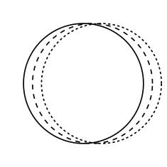
The main purpose of understanding the full asymptotic expansion of solutions in terms of the eigenfunctions of the Hessian around the self-similar solution is to get a deeper understanding of the long-time behavior of solutions. Although we have to keep in mind that our investigation is not fully rigorous in the derivation of the displacement Hessian operator, we will in the following discuss the the role of the smallest eigenvalues and their corresponding eigenfunctions for the convergence towards the attractor $\rho_{*}$ in dimensions $N\geq 2$. We recall that the geodesic curves in the Wasserstein space passing through the Barenblatt solution $\rho_{*}$ along the vector field $\nabla\psi$ are characterized by $\rho_{*}(x)=\det\left(I+s\nabla^{2}\psi\right)\rho_{s}(x+s\nabla\psi)$ (cf. (12)). With this formula at hand, the interpretation of the eigenfunctions as generators of mass transport is immediate. The smallest eigenvalue $\lambda_{10}=1$ corresponds to transitions along the axis $e_{n}$ with $n\in\{1,\dots,N_{1}=N\}$ (see Figure 1a). Indeed, in this case, the eigenfunction is a homogeneous polynomial of degree one, and the displacement is generated by affine perturbations of the identity map $x+sc_{n}e_{n}$ (here, $c_{n}$ denotes a normalizing factor). This fact is in good agreement with the optimal convergence rate of solutions of the porous medium equation to the Barenblatt profile,

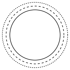
here stated in the Wasserstein topology [22, Theorem 1]. In fact, spatially translated Barenblatt profiles saturate this bound. The eigenfunctions to the second smallest eigenvalue $\lambda_{20}=2$ generate affine transformations on $\mathbbm{R}^{N}$ modulo rotations (Figure 1b). To see this, we observe that $\psi_{20n}$ is a harmonic homogeneous polynomial of degree two, and thus $x+s\nabla\psi=x+sA_{2n}x$ for some symmetric and trace-free matrix $A_{2n}$. In other words, solutions to (3) generated by affine transformations show a rate of convergence of precise order $e^{-2t}$ to the Barenblatt profile. Denzler & McCann [10] give an exact description of the invariant manifold corresponding to these affine perturbations. The role of the next term in the expansion depends on the value of $(m-1)N$. As indicated above, there is a first level crossing of the eigenvalues $\lambda_{\ell 0}$ and $\lambda_{01}$: It is $\lambda_{01}\leq\lambda_{\ell 0}$ precisely for $\ell\geq 1/\alpha$. Eigenfunctions to the eigenvalue $\lambda_{01}$ correspond to isotropic dilations of the Barenblatt profile (see Figure 1d). Indeed, the spherical harmonic $Y_{01}$ degenerates to a constant and $\psi_{011}$ is proportional to $1-(\alpha(m-1)N)^{-1}|x|^{2}$. It follows that $x+s\nabla\psi=(1-cs)x$ for some constant $c$. Such solutions converge with a rate $e^{-t/\alpha}$. The mass transport corresponding to the $(\ell,0)$-modes with $\ell\geq 3$ is less obvious, as the corresponding eigenfunctions $\psi_{\ell 0n}$ are homogenous harmonic polynomials of degree $\ell$. We only discuss the situation where $\ell=3$. In this case, the transformation is quadratic and leads to triangular deformations (see Figure 1c). The rate of convergence is $e^{-3t}$. The deformations corresponding to the remaining eigenvalues can be similarly computed although the complexity of the underlying symmetries is increasing.

We finally remark that the knowledge of spectral properties of the displacement Hessian $\mathcal{H}$, and of the smallest eigenvalue $\lambda_{10}=1$ in particular, immediately yields the sharp spectral gap estimate

for all $\psi\in H^{1}_{\rho_{*}}$. This estimate, was already derived by Otto [22, Sec. 4.4] and builds on McCann’s displacement convexity [19].

We prove Theorem 1 in the remainder of this article: In Subsection 2.2 we show that the displacement Hessian $\mathcal{H}$ can be understood as a self-adjoint operator on $H^{1}_{\rho_{*}}$ (Proposition 1). Moreover, we show that its spectrum is purely discrete (Proposition 2), and thus, the computation of the spectrum reduces to the eigenvalue problem. This requires some preparation. In Subsection 2.3, we treat the case $N\geq 2$ and make a change of variables into spherical coordinates, which has the advantage that the eigenvalue problem reduces to a one-dimensional problem for the radial components of the displacement Hessian. The $N=1$ case is considered in Subsection 2.4, where we split the problem by parity. The resulting eigenvalue problems are solved in Subsection 2.5 for all $N$ simultaneously.

Since $\left.\mathcal{H}\right|_{C^{\infty}(\bar{B}_{1})}$ is nonnegative and symmetric (cf. proof of Proposition 1) and because $C^{\infty}(\bar{B}_{1})$ is densely contained in $H^{1}_{\rho_{*}}$ by Lemma 2 in the appendix, the operator $\left.\mathcal{H}\right|_{C^{\infty}(\bar{B}_{1})}$ is closable in $H^{1}_{\rho_{*}}$ and its closure is still nonnegative and symmetric. We denote this closure again by $\mathcal{H}$. Using the embedding from Lemma 3 in the appendix, one can easily verify that the domain $\mathcal{D}(\mathcal{H})$ of the closed operator is given by (16). In the following we show that $\mathcal{H}$ is self-adjoint and that its spectrum is purely discrete, i.e., it consists only of eigenvalues with finite multiplicity and which do not have a finite accumulation point. For the theory of unbounded operators in general and self-adjointness in particular we refer to [28, Ch. 13] or [29].

The following proposition contains a first statement on the spectrum of $\mathcal{H}$, namely that the spectrum is real and contained in the ray $(0,\infty)$. The first fact is a consequence of self-adjointness, the second one of nonnegativity together with the fact that $\mathcal{H}$ has a bounded inverse (and thus $0$ must be in the resolvent set).

The next result shows that the spectrum consists of eigenvalues only.

In this subsection, we most widely summarize Subsection 4.1 of [9]. As our argumentation for the porous medium equation follows closely the one for the fast-diffusion equation by Denzler & McCann, we entirely skip proofs and refer to [9] for details. An important step in the work of Denzler and McCann is the change of perspective in the spectral analysis of the displacement Hessian $\mathcal{H}$ which comes along with the transformation of the operator into spherical coordinates. In fact, the change of variables into spherical coordinates is motivated by the crucial insight that the displacement Hessian $\mathcal{H}$ and the spherical Laplacian $\Delta_{\mathbbm{S}^{N-1}}$ (i.e., the Laplace–Beltrami operator on the sphere $\mathbbm{S}^{N-1}$) commute. This is basically a consequence of the fact that the evolution commutes with rotations. Consequently, both operators can be simultaneously diagonalized. In particular, as the spectrum of $\Delta_{\mathbbm{S}^{N-1}}$ is well-known, our spectral analysis will reduce to the study of the radial part of $\mathcal{H}$, which amounts to a one-dimensional operator. We remark that this Ansatz is frequently used in the spectral analysis of Schrödinger operators, cf. [21].

We transform $x\in\mathbbm{R}^{N}$ into spherical coordinates, i.e., $x=r\omega$ with $(r,\omega)\in[0,\infty)\times\mathbbm{S}^{N-1}$, and recall that under this transformation, the Laplacian reads

Here $\Delta_{\mathbbm{S}^{N-1}}$ denotes the spherical Laplacian. Since the Barenblatt profile $\rho_{*}$ is a radially symmetric function, i.e., $\rho_{*}=\rho_{*}(r)$, one readily checks that $\mathcal{H}$ and $\Delta_{\mathbbm{S}^{N-1}}$ commute, cf. (14).

The eigenvalues of the spherical Laplacian $\Delta_{\mathbbm{S}^{N-1}}$ are $\mu_{\ell}=\ell(\ell+N-2)$ with multiplicity $N_{\ell}=\frac{(N+\ell-3)!(N+2\ell-2)}{\ell!(N-2)!}$ where $N_{0}=1$. That is,

References

- [1] Abramowitz, M., Stegun, I.A. (Eds.), 1992. Handbook of mathematical functions with formulas, graphs, and mathematical tables. Dover Publications Inc., New York. Reprint of the 1972 edition.
- [2] Angenent, S., 1988. Large time asymptotics for the porous media equation, in: Nonlinear diffusion equations and their equilibrium states, I (Berkeley, CA, 1986). Springer, New York. volume 12 of Math. Sci. Res. Inst. Publ., pp. 21–34. URL: http://dx.doi.org/10.1007/978-1-4613-9605-5_2, doi:10.1007/978-1-4613-9605-5_2.
- [3] Barenblatt, G.I., 1952. On self-similar motions of a compressible fluid in a porous medium. Akad. Nauk SSSR. Prikl. Mat. Meh. 16, 679–698.
- [4] Beals, R., Wong, R., 2010. Special functions. volume 126 of Cambridge Studies in Advanced Mathematics. Cambridge University Press, Cambridge. A graduate text.
- [5] Benamou, J.D., Brenier, Y., 2000. A computational fluid mechanics solution to the Monge-Kantorovich mass transfer problem. Numer. Math. 84, 375–393. URL: http://dx.doi.org/10.1007/s002110050002, doi:10.1007/s002110050002.
- [6] Carrillo, J.A., Toscani, G., 2000. Asymptotic -decay of solutions of the porous medium equation to self-similarity. Indiana Univ. Math. J. 49, 113–142. URL: http://dx.doi.org/10.1512/iumj.2000.49.1756, doi:10.1512/iumj.2000.49.1756.
- [7] Del Pino, M., Dolbeault, J., 2002. Best constants for Gagliardo-Nirenberg inequalities and applications to nonlinear diffusions. J. Math. Pures Appl. (9) 81, 847–875. URL: http://dx.doi.org/10.1016/S0021-7824(02)01266-7, doi:10.1016/S0021-7824(02)01266-7.
- [8] Denzler, J., Koch, H., McCann, R.J., 2012. Higher order time asymptotics of fast diffusion in Euclidean space (via dynamical systems methods). To appear in Mem. Amer. Math. Soc.
- [9] Denzler, J., McCann, R.J., 2005. Fast diffusion to self-similarity: complete spectrum, long-time asymptotics, and numerology. Arch. Ration. Mech. Anal. 175, 301–342. URL: http://dx.doi.org/10.1007/s00205-004-0336-3, doi:10.1007/s00205-004-0336-3.
- [10] Denzler, J., McCann, R.J., 2008. Nonlinear diffusion from a delocalized source: affine self-similarity, time reversal, & nonradial focusing geometries. Ann. Inst. H. Poincaré Anal. Non Linéaire 25, 865–888. URL: http://dx.doi.org/10.1016/j.anihpc.2007.05.002, doi:10.1016/j.anihpc.2007.05.002.
- [11] Evans, L.C., 1998. Partial differential equations. volume 19 of Graduate Studies in Mathematics. American Mathematical Society, Providence, RI.
- [12] Friedman, A., Kamin, S., 1980. The asymptotic behavior of gas in an -dimensional porous medium. Trans. Amer. Math. Soc. 262, 551–563. URL: http://dx.doi.org/10.2307/1999846, doi:10.2307/1999846.
- [13] Groemer, H., 1996. Geometric applications of Fourier series and spherical harmonics. volume 61 of Encyclopedia of Mathematics and its Applications. Cambridge University Press, Cambridge. URL: http://dx.doi.org/10.1017/CBO9780511530005, doi:10.1017/CBO9780511530005.
- [14] Hebey, E., 1999. Nonlinear analysis on manifolds: Sobolev spaces and inequalities. volume 5 of Courant Lecture Notes in Mathematics. New York University Courant Institute of Mathematical Sciences, New York.
- [15] Kamenomostskaya, S., 1973. The asymptotic behavior of the solution of the filtration equation. Israel J. Math. 14, 76–87.
- [16] Kamin, S., 1975/76. Similar solutions and the asymptotics of filtration equations. Arch. Rational Mech. Anal. 60, 171–183.
- [17] Kamin, S., Vázquez, J.L., 1988. Fundamental solutions and asymptotic behaviour for the -Laplacian equation. Rev. Mat. Iberoamericana 4, 339–354.
- [18] Koch, H., 1999. Non-Euclidean singular integrals and the porous medium equation. Ph.D. thesis. Habilitation thesis, Universität Heidelberg, Germany.
- [19] McCann, R.J., 1997. A convexity principle for interacting gases. Adv. Math. 128, 153–179. URL: http://dx.doi.org/10.1006/aima.1997.1634, doi:10.1006/aima.1997.1634.
- [20] Newman, W.I., 1984. A Lyapunov functional for the evolution of solutions to the porous medium equation to self-similarity. I. J. Math. Phys. 25, 3120–3123. URL: http://dx.doi.org/10.1063/1.526028, doi:10.1063/1.526028.
- [21] Nikiforov, A.F., Uvarov, V.B., 1988. Special functions of mathematical physics. Birkhäuser Verlag, Basel. A unified introduction with applications, Translated from the Russian and with a preface by Ralph P. Boas, With a foreword by A. A. Samarskiĭ.
- [22] Otto, F., 2001. The geometry of dissipative evolution equations: the porous medium equation. Comm. Partial Differential Equations 26, 101–174. URL: http://dx.doi.org/10.1081/PDE-100002243, doi:10.1081/PDE-100002243.
- [23] Otto, F., Westdickenberg, M., 2005. Eulerian calculus for the contraction in the Wasserstein distance. SIAM J. Math. Anal. 37, 1227–1255 (electronic). URL: http://dx.doi.org/10.1137/050622420, doi:10.1137/050622420.
- [24] Pattle, R.E., 1959. Diffusion from an instantaneous point source with a concentration-dependent coefficient. Quart. J. Mech. Appl. Math. 12, 407–409.
- [25] Rainville, E.D., 1971. Special functions. first ed., Chelsea Publishing Co., Bronx, N.Y.
- [26] Rainville, E.D., 1972. Intermediate differential equations. second ed., Chelsea Publishing Co., New York.
- [27] Ralston, J., 1984. A Lyapunov functional for the evolution of solutions to the porous medium equation to self-similarity. II. J. Math. Phys. 25, 3124–3127. URL: http://dx.doi.org/10.1063/1.526029, doi:10.1063/1.526029.
- [28] Rudin, W., 1991. Functional analysis. International Series in Pure and Applied Mathematics. second ed., McGraw-Hill Inc., New York.
- [29] Schmüdgen, K., 2012. Unbounded self-adjoint operators on Hilbert space. volume 265 of Graduate Texts in Mathematics. Springer, Dordrecht. URL: http://dx.doi.org/10.1007/978-94-007-4753-1, doi:10.1007/978-94-007-4753-1.
- [30] Vázquez, J.L., 2003. Asymptotic behaviour for the porous medium equation posed in the whole space. J. Evol. Equ. 3, 67–118. URL: http://dx.doi.org/10.1007/s000280300004, doi:10.1007/s000280300004. dedicated to Philippe Bénilan.
- [31] Vázquez, J.L., 2006. Smoothing and decay estimates for nonlinear diffusion equations. volume 33 of Oxford Lecture Series in Mathematics and its Applications. Oxford University Press, Oxford. URL: http://dx.doi.org/10.1093/acprof:oso/9780199202973.001.0001, doi:10.1093/acprof:oso/9780199202973.001.0001. equations of porous medium type.
- [32] Vázquez, J.L., 2007. The porous medium equation. Oxford Mathematical Monographs, The Clarendon Press Oxford University Press, Oxford. Mathematical theory.
- [33] Villani, C., 2003. Topics in optimal transportation. volume 58 of Graduate Studies in Mathematics. American Mathematical Society, Providence, RI. URL: http://dx.doi.org/10.1007/b12016, doi:10.1007/b12016.
- [34] Villani, C., 2009. Optimal transport. volume 338 of Grundlehren der Mathematischen Wissenschaften [Fundamental Principles of Mathematical Sciences]. Springer-Verlag, Berlin. URL: http://dx.doi.org/10.1007/978-3-540-71050-9, doi:10.1007/978-3-540-71050-9. old and new.
- [35] Zel′dovič, Y.B., Barenblatt, G.I., 1958. Asymptotic properties of self-preserving solutions of equations of unsteady motion of gas through porous media. Dokl. Akad. Nauk SSSR (N.S.) 118, 671–674.
- [36] Zel′dovič, Y.B., Kompaneec, A.S., 1950. On the theory of propagation of heat with the heat conductivity depending upon the temperature, in: Collection in honor of the seventieth birthday of academician A. F. Ioffe. Izdat. Akad. Nauk SSSR, Moscow, pp. 61–71.