A Real-time Group Auction System for Efficient Allocation of Cloud Internet Applications

A cloud user $i$ submits a bid defined by $b_{i}=(\vec{d_{i}},\vec{\ell_{i}},v_{i})$ where $\vec{d_{i}}=(d_{i}^{1},d_{i}^{2},\ldots,d_{i}^{K})^{T}$ is a demand, and $d_{i}^{k}$ indicates the number of instances of type $k$. $\vec{\ell_{i}}=(\ell_{i},t_{i}^{s},t_{i}^{e})^{T}$ is a demand period where $\ell_{i}$ indicates a length of time that the user $i$ wants to reserve a bundle of the instances between starting time $t_{i}^{s}$ and ending time $t_{i}^{e}$. For example, $\vec{\ell_{i}}=(3,2,8)$ indicates that user $i$ requests instances for 3 time slots (that do not have to be consecutive) between time 2 and time 8, each of the time slots reserves $\vec{d_{i}}$ instances. We define $t_{i}^{d}\equiv t_{i}^{e}-\ell_{i}$ and call it the deadline by which the instances should be assigned to satisfy the demand. $v_{i}$ is user $i$’s valuation for the demand as a bidding price, which indicates the maximum price that is acceptable for the user to buy the requesting instances.

A cloud provider $j$ submits an offer defined by $o_{j}=(\vec{s_{j}},\vec{w_{j}},Q_{j})$ where $\vec{s_{j}}=(s_{j}^{1},s_{j}^{2},\ldots,s_{j}^{K})^{T}$ is a supply and $s_{j}^{k}$ indicates the number of instances of type $k$ that provider $j$ can provide per time slot. $\vec{w_{j}}=(t_{j}^{s},t_{j}^{e})^{T}$ is a supply period²² 2 We formalize the supply period as variables whose values are different for different providers. The providers might be personal providers or small companies that supply their resources for limited time periods [25] while large providers [1] do not limit the supply period in general.. $w_{j}\equiv t_{j}^{e}-t_{j}^{s}$ denotes a length of time that a provider is able to provide the instances between $t_{j}^{s}$ and $t_{j}^{e}$. $Q_{j}$ is provider $j$’s valuation³³ 3 In practice, the provider’s valuation to an instance is determined based on several factors such as the value of applications to users, the running cost of servers, and other competing providers. It is beyond our work in this paper to understand how providers set their own valuations. For simplicity, we assume that the valuations are pre-determined. for the supply as an offering price curve, which indicates the minimum of a unit price of the offered instances that the provider wishes to sell. It is defined by a set of vectors over different number of instances and instance types as follows: $Q_{j}=(\vec{q}_{j}^{1},\vec{q}_{j}^{2},\ldots,\vec{q}_{j}^{K})$ where $\vec{q}_{j}^{k}=(q_{j}^{k}[1],\ldots,q_{j}^{k}[n_{j}^{k}])^{T}$, and $q_{j}^{k}[n]$ indicates the offering price when $n$ instances of type $k$ are sold by provider $j$, and $q_{j}^{k}[0]=+\infty$. $\vec{q}_{j}^{k}$ holds a condition $q_{j}^{k}[1]\geq\cdots\geq q_{j}^{k}[n_{j}^{k}]$. Let $Q_{j}[\vec{n_{j}}]$ denote an extraction of the price curve when $\vec{n_{j}}=(n_{j}^{1},n_{j}^{2},\ldots,n_{j}^{K})$ instances are sold, which is represented as a row vector $Q_{j}[\vec{n_{j}}]=(q_{j}^{1}[n_{j}^{1}],q_{j}^{2}[n_{j}^{2}],\ldots,q_{j}^{K}[n_{j}^{K}])$.

In the proposed system, users and providers can form coalitions to gain benefits in terms of resource price and resource utilization efficiency. Figure 2 shows two examples explaining two types of cooperation. One, illustrated in Figure 2(a), is the case that multiple users request resources of the same provider to lower the instance price. Another, illustrated in Figure 2(b), is the case that multiple providers supply resources to meet the same user’s request. An edge-dotted line indicates the allocation of a user and a provider. A shaded box indicates the allocated instances. The height of the box represents the number of instances.

For the first type, multiple cloud users are allowed to form a group, i.e., we call a user coalition, and request instances of the same provider in order to buy the instances at a discounted price. For example, when two users request 10 instances ($d_{1}=4$ and $d_{2}=6$) as a coalition, a provider’s offering price changes from $q[4]$ (or $q[6]$) to $q[10]$ where $q[4]=q[6]>q[10]$. However, a cooperation may incur a delay of the instance allocation because different users have different demand periods. Figure 2(a) explains the delay (denoted by an arrow) of User 1 forming a coalition with User 2. Instances for User 1 could be allocated from time $t_{1}^{s}$.

For the second type, multiple cloud providers are also allowed to form a group, i.e., we call a provider coalition. The providers in the same coalition can share users’ demands to meet their requests. For doing this, users’ instances can be migrated from one provider to another as indicated by a down arrow in Figure 2(b). This cooperation enables the effective use of the residual resources and improves their resource utilization. However, the cooperation may incur a cost for the instance migration. For example, during migration, the degradation of application performance (e.g., throughput and response time) can be considered as the cost.

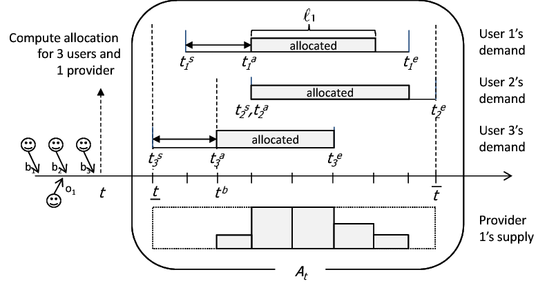
Denote $B_{t}$ as a set of bids and $O_{t}$ as a set of offers that the controller retains at time $t$, respectively. A demand period for demands in $B_{t}$ is specified by $\underline{t}=\min\{t_{i}^{s}|t_{i}^{s}\in b_{i},\forall b_{i}\in B_{t}\}$ and $\overline{t}=\max\{t_{i}^{e}|t_{i}^{e}\in b_{i},\forall b_{i}\in B_{t}\}$. The allocation at time $t$ is defined by a three-dimensional ($|B_{t}|\times|O_{t}|\times(\overline{t}-\underline{t})$) matrix $A_{t}\equiv[a_{ijs}]$ for $i=1,\ldots,|B_{t}|$, $j=1,\ldots,|O_{t}|$, $s=\underline{t}+1,\ldots,\overline{t}$ where a binary variable $a_{ijs}$ is 1 if user $i$’s demand is allocated to provider $j$ at time slot $s$, and 0 otherwise. We assume that a user’s demand is satisfied when all of the numbers of requested instances is allocated. Also, we assume that user’s instances are allocated to one provider at each time slot. Thus, the system does not consider the partially allocated instances. We denote the optimal allocation by $A_{t}^{*}\equiv[a_{ijs}^{*}]$, where the method to obtain it will be discussed in the next section.

Given the allocation $A_{t}$, the controller computes the best time to announce the allocation information (denoted by in Figure 1). We call it bid closing time, which is denoted as $t^{b}=\min_{A_{t}}\{t_{i}^{a}\}$ where $t_{i}^{a}$ is the earliest time that user $i$’s demand is allocated according to $A_{t}$. Figure 3 illustrates an example of allocation for three users and one provider over the demand period of eight time slots. In this example, the allocation is $A_{t}=[\vec{a}_{11s},\vec{a}_{21s},\vec{a}_{31s}]=[(0,0,0,1,1,1,0,0)^{T},(0,0,0,1,1,1,1,0)^{T},(0,0,1,1,1,0,0,0)^{T}]$, the demand period is $\underline{t}=t_{3}^{s}$ and $\overline{t}=t_{2}^{e}$, and the bid closing time is $t^{b}=t_{3}^{a}$.

Users and providers are allowed to trade their instances in their own groups. Given bids and offers in each group, the instance allocation of the group is formulated as an optimization problem to maximize the social welfare, i.e., the total utilities of the users and providers.

The utility of user $i$ in group $G$ with the allocation $A_{t}$ is given by

where $c_{i}$ is a final charge to user $i$, $v_{is}\equiv\frac{v_{i}}{\ell_{i}}$ is user $i$’s valuation to instances $\vec{d_{i}}$ at time slot $s$, and $p_{ijs}$ is a trading price for the instances $\vec{d_{i}}$ between user $i$ and provider $j$ at time slot $s$.

The utility of provider $j$ in group $G$ with the allocation $A_{t}$ is given by

where $r_{j}$ is a provider $j$’s revenue and $v_{j}$ is a provider $j$’s valuation to the total amount of supplied instances $D_{js}^{k}=\sum_{i\in G^{u}}a_{ijs}\cdot d_{i}^{k}$ for $k=1,\ldots,K$. Therefore, the instance allocation $A=[a_{ijs}]$ in group $G$ is formulated as follows:

subject to

for $\forall i\in G^{u}$, $\forall j\in G^{p}$, $\underline{t}<s\leq\overline{t}$, $1\leq k\leq K$ where $\underline{t}=\min\{t_{i}^{s}|\forall i\in G^{u}\}$, $\overline{t}=\max\{t_{i}^{e}|\forall i\in G^{u}\}$.

Thus, the social welfare optimization problem is formulated to find the instance allocation that maximizes the total utilities of users and providers (Equation (3)) under constraints (4)-(6) of the amount of supplied instances and about the allocation. Constraint (4) guarantees that the total number of requested/allocated instances does not exceed the total number of supplied instances. Constraint (5) indicates that a user’s demand is satisfied when all of the requested instances are allocated, which is specified by a binary variable $x_{i}$. Constraint (6) indicates that user’s instances are allocated to only one provider at each time slot, which is specified by a binary variable $y_{is}$. Thus, the system does not consider the partially allocated instances.

The formulated binary integer programming is known to be NP-hard that the number of different allocations to be evaluated exponentially increases as the numbers of users and providers increase. We propose a dynamic algorithm to find the nearly optimal solution in a reasonable time.

Algorithm 1 shows the dynamic algorithm to find the nearly optimal solution given bids $B_{t}$ and $O_{t}$ at time $t$. The key idea of this algorithm is to give higher allocation priority to users who bid with higher valuation and providers who offer with lower valuation. Besides, the algorithm allocates instances from the time slot that more users request their instances to the time slots that less users request because providers are likely to offer a discount price in such time slot.

At the beginning (Lines 1-9), the algorithm checks the users’ demand periods and counts how many users request their instances over different time slots from $\underline{t}+1$ to $\overline{t}$. $C$ is a count vector, whose element $C_{s}$ indicates the number of users whose demand periods include the time slot $s$. Pos is a mapping between users and providers, whose element Pos_i is a provider id that a user $i$ is assigned to. Pos${}_{i}=0$ means that a user $i$ is not mapped to any providers.

In the following loop (Lines 12-37), the algorithm finds the allocation $A_{t}$ by starting to consider time slot $s$ in descending order of the counts $C$ (Line 12). The first subloop (Lines 16-30) computes the best mapping between users and providers at time slot $s$. According to the total number of instances requested by users in the same group (Line 21), the users with relatively higher valuations are preferably assigned (Line 30) to providers with relatively lower valuations if such providers $j^{*}$ exist (Line 23). If there is no such providers, then users consider other providers in different groups (Line 26). If users cannot find any providers, then their demands cannot be assigned at this time slot (Line 25). The second subloop (Lines 32-36) updates the recent allocation based on the computed mapping. Once all instances requested by a user are mapped, the user $i$ and his bid $b_{i}$ are excluded (Line 36).

Based on the allocation, the trading price is determined in a way that the social welfare is distributed to participants in proportional to their contributions, i.e., valuations. First, the controller computes the total price charged to users for each group $G$. The price at time slot $s$ is given as follows:

where $\kappa\in[0,1]$. $\kappa$ is set to 0.5 in this paper to give users and providers the fairness.

Second, the users in $G$ divide the total price $p_{Gs}$ in weights proportional to the user’s valuation. Hence, the price for user $i$ is defined by

where $V_{s}=\sum_{i\in G^{u}}v_{is}$ is the total valuation of users in $G$.

Consequently, the cost (i.e., the total charge) for user $i$ is

and the revenue for provider $j$ is

The payoff for user $i$ is designed as the difference between the utility and the delaying penalty by forming a group and defined as follows:

where $A_{t}^{*}=\arg\max_{A_{t}}\mathcal{U}(G,A_{t})$, and the delaying penalty is defined by

The actual cost $C^{d}$ may differ according to different participants, applications, and time slots. However, for simplicity, we assume that the actual cost is proportional to the delay.

Similarly, the payoff for provider $j$ is designed as the difference between the utility and the additional cost by migrating instances and defined as follows:

where the cost for instance migration is defined by

The migration cost $C^{m}$ also differs among providers. However, we assume the value to be a constant for all providers.

For constructing a group formation, we introduce an algorithm that allows users and providers to make the group formation decisions for selecting which groups (i.e., providers) to join and which users to accept. The decisions are called migrating, merging, and splitting.

Migrating: Given a group structure $\Omega=(\Pi=(G_{1},\ldots,G_{m},\ldots,G_{M}),L)$, any user $i\in G_{m}^{u}$ decides to migrate from its current associated provider $j\in G_{m}^{p}$ to another provider $j^{\prime}\in G_{m^{\prime}}^{p}$ where $m\neq m^{\prime}$ if the following condition is satisfied:

The condition (23) guarantees for a user to improve its own payoff by performing the migrating decision. For every single migration of user $i$, the group structure $\Omega$ is updated to $\Omega^{\prime}=(\Pi^{\prime},L^{\prime})$ where $\Pi^{\prime}=(\Pi\backslash\{G_{m},G_{m^{\prime}}\})\cup\{G_{m}\backslash\{i\},G_{m^{\prime}}\cup\{i\}\}$, and $L^{\prime}=L\backslash(i,j)\cup(i,j^{\prime})$.

Merging: Multiple groups $G_{m}\in\Pi_{s}$, a subset of $\Pi$ (i.e., $\Pi_{s}\subseteq\Pi$) can collectively form a single group $G_{m^{\prime}}^{\dagger}$ if the following conditions are satisfied:

where $G_{m^{\prime}}^{\dagger}=\cup_{\Pi_{s}}G_{m}$. The first condition in (24) guarantees for a provider to improve its own payoff by performing the merging decision. The other conditions guarantee that none of the other members (both users and providers) in the newly formed group decreases their payoffs by the merging decision. For every single merging decision, the group structure $\Omega$ is updated to $\Omega^{\dagger}=(\Pi^{\dagger},L)$ where $\Pi^{\dagger}=(\Pi\backslash\{\forall G_{m}\in\Pi_{s}\})\cup G_{m^{\prime}}^{\dagger}$ where $|\Pi^{\dagger}|<|\Pi|$.

Splitting: Given the original group $G_{m}$, members in this group can collectively split into multiple groups $G_{m^{\prime}}^{\ddagger}$, whose set after the splitting is denoted by $\Pi_{s}^{\ddagger}$, if the following conditions are satisfied:

where $G_{m}=\cup_{\Pi_{s}^{\ddagger}}G_{m^{\prime}}^{\ddagger}$ and for all $G_{m^{\prime}}^{\ddagger}$ there exist $(i,j)\in L$ such that $i\in G_{m^{\prime}}^{\ddagger u}$ and $j\in G_{m^{\prime}}^{\ddagger p}$. The first condition in (27) guarantees for a provider to improve its own payoff by performing the splitting decision. The other conditions guarantee that none of the members in newly formed groups decreases their payoffs by the splitting decision. For every single splitting decision, the group structure $\Omega$ is updated to $\Omega^{\ddagger}=(\Pi^{\ddagger},L)$ where $\Pi^{\ddagger}=(\Pi\backslash G_{m})\cup\{\forall G_{m^{\prime}}^{\ddagger}\in\Pi_{s}^{\ddagger}\}$ where $|\Pi^{\ddagger}|>|\Pi|$.

Figure 4(b) illustrates example group structures after migrating, merging, or splitting decision given the group structure in Figure 4(a). For example, after the migration by u₃, the group structure changes to $G_{0}=\{4\},G_{1}=\{\{1,2\},\{1,2,4\}\},G_{2}=\{\{3,5\},\{3\}\}$, and $L=\{(1,2),(2,1),(3,3),(4,0),(5,3)\}$. After the merging by p₂, the groups 1 and 2 become one group $G_{1}=\{\{1,2,3,5\},\{1,2,3,4\}\}$ with the same associated links. After the splitting by p₂, the group 1 is splitted into $G_{1}=\{\{2\},\{1,4\}\},G_{3}=\{\{1,3\},\{2\}\}$ with the same associated links.

Algorithm 2 shows a pseudocode of the proposed group formation algorithm that finds a stable group structure. At the beginning (Line 3), the algorithm initializes a group structure $\Omega$ by randomly setting groups and associated links (Lines 4 and 5 in Algorithm 3). A randomly initialized group structure converges to the stable group structure for participants by repeatedly selecting distributed decisions (Lines 9, 13, and 16) that improve both users and providers’ payoffs. During the iterations (Lines 4-18), a history set $H$ is maintained, which stores the groups that are formed or evaluated in the past. To compute the payoffs, Algorithm 1 is executed. The algorithm stops when none of the participants changes their groups (Line 18).