An Efficient and Optimal Filter for Identifying Point Sources in Millimeter/Sub-Millimeter Wavelength Sky Maps
Abstract
A new technique for reliably identifying point sources in millimeter/sub-millimeter wavelength maps is presented. This method accounts for the frequency dependence of noise in the Fourier domain as well as non-uniformities in the coverage of a field. This optimal filter is an improvement over commonly-used matched filters that ignore coverage gradients. Treating noise variations in the Fourier domain as well as map space is traditionally viewed as a computationally intensive problem. We show that the penalty incurred in terms of computing time is quite small due to casting many of the calculations in terms of FFTs and exploiting the absence of sharp features in the noise spectra of observations. Practical aspects of implementing the optimal filter are presented in the context of data from the AzTEC bolometer camera. The advantages of using the new filter over the standard matched filter are also addressed in terms of a typical AzTEC map.
Keywords:
Data Analysis and Techniques, Astrophysical DataI Introduction
The discovery and study of sub-millimeter galaxies, or SMGs, has become a key enterprise within millimeter/sub-millimeter (mm/sub-mm) astronomy over the past decade or so [7, see review by]. With bolometric luminosities and star formation rates yr-1 , SMGs represent some of the most luminous galaxies in the early Universe. The strong negative -correction at m means that a galaxy of a given luminosity will be equally detectable in a flux-limited survey from . A deep, wide-area survey at mm/sub-mm wavelengths is thus a sensitive probe of starburst galaxies from the epoch at which they first turn on through the peak of star formation activity in the Universe at . Several papers have reported on the source counts of SMGs detected at m [e.g. 10, 5, 22, 20, 16, and references therein], which provide strong constraints on the evolutionary history of massive galaxies [4, 19, 6, e.g.]. SMG surveys from single-dish telescopes also provide a catalog of interesting targets to follow-up with higher angular resolution imaging of the dust and molecular gas in these objects, which inform on the physical processes that trigger and maintain the starbursts in these galaxies.
An important criterion for the success of such surveys is the design of a data analysis scheme that can reliably identify SMG candidates on sky maps. It is especially important to minimize the rate of false detections because they can result in a waste of valuable time and resources in follow-up observations. But reliably identifying astronomical signal in mm/sub-mm maps is a difficult task because these maps are inherently low in signal/noise due to atmospheric contamination, instrument noise, and the high confusion limit of surveys from typical mm/sub-mm telescopes (10 m diameter). In the wide field surveys designed to detect SMGs, they usually appear as point sources much smaller than the angular resolution of the telescopes used. A simple approach to identify point sources that is used by standard data analysis packages [see 17, for example] is: 1) smooth the signal map by convolving it with the point spread function (PSF); 2) assume that the errors associated with pixels are uncorrelated and propagate them through the convolution; and 3) select the peaks in the smoothed map based on the per-pixel signal/noise determined from steps 1) and 2). This reduces high-frequency signal variations between adjacent pixels and thus increases the signal/noise for point-source detection.
However, there are two general problems with real mm/sub-mm maps that renders the above procedure inadequate for reliably identifying point sources. First, the noise in these maps is generally not white; it is more pronounced on larger scales or at low (spatial) frequencies. This effect, which gives rise to pixel-pixel correlations, is due mainly to drifts in atmospheric and/or instrumental conditions. In mm/sub-mm astronomy, this problem is usually treated with a “matched filter” implemented in the Fourier domain [18, 3, 21, 2, 14, 9, e.g.]. However, this filtering technique is optimal only in the case of uniform coverage, which brings up the second problem with real mm/sub-mm maps: the coverage of a field is non-uniform in general. Because these observations are usually carried out by scanning an array of detectors across the field of interest, variations in atmospheric conditions or detector noise during the scan are often responsible for this non-uniformity. With commonly used schemes such as raster- or Lissajous-scanning, coverage also tends to decrease smoothly from the center to the edges of the map.
The correct way to deal with both these problems involves the construction and inversion of a pixel-pixel noise covariance matrix. This path can be extremely challenging computationally for maps containing pixels. Therefore, a common strategy is to pick out a region of the map that has essentially uniform coverage and then apply the standard matched filter to it. Even when a near-uniform region exists, ignoring small coverage variations within it can have a noticeable effect, as we will show below. Furthermore, despite gradients, the coverage may be deep enough near the edges of the map to identify bright sources with high significance, and these “border” regions can often cover a significant area compared to the near-uniform region. In some cases, significant coverage gradients are unavoidable due to difficult observing conditions or an observing strategy where a mosaic of small maps are stitched together [8, 10, 1, for example, see]. A truly optimal analysis would help improve the reliability with which point-source candidates are identified in all regions of a map despite coverage gradients.
In this paper, we present an algorithm that addresses non-uniform coverage as well as low-frequency noise in a computationally efficient manner. This technique is designed to be optimal in the regime where blending of resolved sources is negligible. The work presented here is an extension of the standard data reduction tools used for point-source extraction in maps taken with the 1.1 mm bolometer array camera, AzTEC [23]. While this builds on the existing AzTEC reduction pipeline [15, 14], the principles are generic to any scan-data from mm/sub-mm arrays. In section II we present the formal methodology that will be used to identify point sources and to estimate their brightness. Essentially, this method involves a least-squares fit of the PSF to every point on the map. In section III, we demonstrate that, for the case of uniform coverage, the fit paradigm converges to the familiar and computationally efficient matched filter routinely used in point-source searches. In section IV, we develop an implementation of the pixel-by-pixel fit that can efficiently handle the case of non-uniform coverage. Then, in section V, we discuss the practicalities of applying this technique to AzTEC data. Finally, in section VI, we conclude by discussing the performance and scope of the optimal filter introduced here.
II The Method
We leverage our knowledge of the shape of isolated point sources in our maps to construct an optimal or wiener filter using the point spread function (PSF) as the template. Applying this filter to the map is formally equivalent to centering the PSF on each pixel of the map and fitting for the best-fit amplitude [17]. In our case, we store the best fit amplitude at each pixel in a separate map which we will refer to as the filtered signal map. In addition, we construct a new map of the same dimensions as the signal map which contains 1/error2 estimates of the best fit amplitudes. This map will be referred to as the filtered coverage map. These maps, augmented by noise realizations of the field, are the primary inputs to the identification of point sources.
II.1 AzTEC data as an example
AzTEC is a 144-element semiconductor-type bolometer array that imaged the sky at 1.1-mm wavelength over two successful observing campaigns: one using the 15-m James Clark Maxwell Telescope (JCMT) in Hawaii from 2005-2006 [23], and the other using the 10-m Atacama Sub-millimeter Telescope Experiment (ASTE) in the Atacama desert of Chile from 2007-2008 [12]. Over these two observing runs, close to a hundred fields were mapped, and each map comprises 100,000 pixels or more. Therefore, computational speed was an important consideration when developing this algorithm. Computational speed will be even more important for newer and upcoming mm/sub-mm observatories like the Large Millimeter Telescope and CCAT that can image the sky at even faster rates with higher angular resolution.
 |
 |
| (a) | (b) |
To illustrate the starting point for the filtering process, we present in Fig. 1 an unfiltered AzTEC signal map and the corresponding coverage map. In the AzTEC data analysis, coverage maps have units of 1/Jy2 and are filled with estimates of 1/error2 at each pixel. In Fig. 1 and throughout the rest of this paper, we will use maps and plots related the AzTEC-ASTE data on a region centered around the high-redshift quasar SDSSJ1030+0524 to illustrate our points. This data set consists of 45 observations of the field, each lasting about forty minutes, carried out over November 2008. Scientific results from this AzTEC-ASTE field are published in Humphrey et al. [13] and Zeballos [26]. These data were taken by scanning the AzTEC array in a Lissajous pattern, and results in a map with deepest coverage in the center, and decreasing coverage toward the edges of the map.
II.2 Assumptions
Two assumptions, both of which are generally applicable to most observations, are critical for the efficient implementation of the process described below. They are:
1. The effective PSF does not change with location on the map. We represent the PSF by the two-dimensional function . The value of this function at the ’th pixel when the PSF is centered on the ’th pixel will be denoted by where and are 2-d vectors that specify the locations of the ’th and ’th pixels, respectively. We note that while this assumption is explicitly not valid for some instruments (e.g., the Chandra X-ray telescope), this is a reasonable assumption for many imaging instruments.
2. Noise-induced correlations between two pixels, hereafter denoted depend only on the distance between the pixels. That is, neither the location of the two pixels on the map nor their relative orientation determines the correlation in their noise. In such cases, may be conveniently expressed as the inverse Fourier transform (IFT) of the power spectral density (PSD) of noise in the map. If we denote the PSD by where is a 2-d vector in the Fourier domain of the map,
| (1) |
where is the total number of pixels in the map, and the sum is over all vectors . (Appendix A contains a brief description of the discrete Fourier transform conventions and their corollaries used here.)
In Eq. 1, is a normalized form of the PSD that satisfies so that the diagonal elements of the correlation matrix evaluate to 1. Note that for a completely flat PSD () the correlation matrix is diagonal. In most observations the noise PSD varies smoothly with and has broad features rather than narrowly peaked ones (see Fig. 3, for example). In such cases the correlation matrix is band-diagonal (i.e., when is large). This is a property that we will exploit below in our pursuit of computational efficiency.
II.3 An optimal filter via a generalized least-squares fit
We implement the optimal filter by minimizing the quantity
| (2) |
for each pixel, , in the map where and denote the value of the unfiltered signal map at the ’th and ’th pixels, is the amplitude of the fitted PSF, and is an weight matrix whose calculation is described below. The summations in Eq. 2 are over all pixels of the map. Eq. 2 is minimized when
| (3) |
For least-squares fits, the minimum variance choice of the weight matrix is where is the pixel-pixel noise covariance matrix (i.e. the map’s covariance in the absence of signal). In this case, the calculated in Eq. 2 is drawn from a true distribution with degrees of freedom. The elements of are
| (4) |
where and are the standard deviations of noise in the -th and -th pixels respectively. Note that the diagonal elements, evaluate to as they should.
The elements of the weight matrix can then be calculated as
| (5) |
Using Eq. A5 of Appendix A, it is straightforward to verify that Substituting the above form of into Eq. 3, we may express the numerator and denominator of Eq. 3 as
| (6) | |||||
| (7) |
In practice, we form separate “maps” corresponding to and because the latter is useful by itself (see below). In doing so, the nested sums of Eq. 6 and Eq. 7 will be recognized as Fourier transforms, allowing us to benefit from the efficiency of the FFT algorithm. The element-by-element ratio of these two, forms the filtered signal map.
II.4 Error propagation
The error in our estimate of which we denote , is the rms deviation of the best fit PSF amplitude, , from the actual amplitude, , of a point source that is centered on the ’th pixel. i.e. To estimate we consider the influence of a point source located at the ’th map pixel on a neighboring pixel
| (8) |
As mentioned above, we recognize that the possibility of other resolved sources being quite close to pixel (source blending) is ignored in Eq. 8 and must be treated iteratively. Using Eq. 8 for and Eq. 3 for our estimate for is
| (9) |
and since the above expression simplifies to
| (10) |
Thus, when the optimal is used, no extra steps are needed to evaluate as already exists from generating the filtered signal map.
II.5 Source significance and goodness of fit
The filtered signal-to-noise map, filled with values can be used to both identify and locate sources of high significance. Rewriting Eq. 2 in a more convenient form using Eq. 3 and Eq. 10 gives
| (11) |
Because the first term in Eq. 11 is common to all pixels the second term is a direct indication of the goodness of fit at the ’th pixel. Thus, the locations of peaks in the signal-to-noise map, , provide the best estimates of point-source positions on the map.
III The case of uniform coverage
It is instructive to first consider the case of uniform coverage. In this case, in Eqs. 6 and 7 and so can be moved outside the summations. The sums over and are then recognized as Fourier transforms (FTs) of the signal map () and the PSF (), leading to the result that
| (12) |
where and are the 2-d FTs of and respectively. The above expression is the familiar “matched filter” that is commonly used in mm/sub-mm astronomy for identifying point sources [18, 3, 21, 2, 9, for example, see] and is essentially a band-pass filter in the sense that the data () are low-pass filtered by the PSF and high-pass filtered by as the PSD usually displays a -type trend with spatial frequency. The denominator of Eq. 12 simply provides the correct normalization. What Eq. 12 shows is that the point-source finding technique of fitting a PSF to each map pixel converges to the conventional matched filter in the case of uniform coverage.
Another important feature of Eq. 12 is that, in terms of the FTs and the numerator and the denominator are each reduced to a single sum of terms and the total calculation scales as rather than as . As for having to evaluate at each pixel, we note that (1) the denominator needs to be evaluated just once for all pixels and (2) a “map” of the numerator is simply an inverse Fourier transform (IFT). Therefore, the entire filtering process can be accomplished with calculations. On a desktop computer with a 2.5 GHz Intel processor and 4.7 GB of RAM, the pixel map of Fig. 1 can be filtered according to Eq. 12, using the IDL programming language, in under 0.5 seconds.
Using the standard matched filter is similar to performing a simple least squares minimization under the approximation that all pixels in the map have the same uncertainty. If the underlying noise is not uniform and this method is used, one must recognize that and so the error distributions of the cannot be formally calculated as given in Eq. 10 above.
IV The case of non-uniform coverage
We show here that, in a map with non-uniform coverage, it is possible to treat the general problem of point source identification in a computationally efficient, yet mathematically sound way. We find that loosening the assumption of uniform coverage results in an increase in computation time that is noticeable but inconsequential in practical terms. As the calculation of turns out to be more complex than the calculation of we tackle first.
IV.1 The calculation of
as expressed in Eq. 6, can be calculated through a sequence of FTs and IFTs. We motivate this by casting Eq. 6 in a more suggestive manner:
| (13) |
Proceeding from the innermost parentheses outward, the steps needed to calculate are:
- 1.
Form a new map filled with values
- 2.
The calculation within the innermost parentheses can be recognized as a Fourier Transform (see Appendix A). Therefore, form
- 3.
Similarly, the calculation within the next set of parentheses is an IFT. Thus, form
- 4.
Form a new matrix which is filled with values The sum over in Eq. 13 is simply a convolution of by the PSF
- 5.
As it is computationally advantageous to carry out this convolution in the Fourier domain, calculate and
- 6.
Finally,
There are 5 FFTs in this sequence. On the same standard desktop PC described in Section III, the complete computation sketched above takes less than one second for a -pixel map.
IV.2 The calculation of
The calculation of the denominator, , is more involved than the numerator as there are no simplifications that allow to reduce to a series of Fourier Transforms. As a result, a full calculation of requires of calculations. In the case of the -pixel map used here, this takes about seven hours on the basic computing platform considered in Section III. We can do better though. Below we give an approximation to with an accuracy better than 0.1% that takes minutes to calculate.
Our Approximation of makes use of the band-diagonal nature of the noise correlation matrix or, equivalently, the smoothly varying nature of as discussed in section II. We start by defining a new vector, and re-writing Eq. 7 as
| (14) |
where is the IFT of or
| (15) |
To clearly demonstrate that the sum over is a convolution, we define the new functions and as follows:
| (16) | |||||
| (17) |
Thus, (or ) is the product of (or ) and a version of (or ) that is shifted by the vector Using these definitions, we may express as
| (18) |
which is recognizable as a convolution. Finally, using the discrete convolution theorem (see Eq. A5), we find that
| (19) |
The advantage of casting in the form of Eq. 19 is the following: is narrowly peaked near because it is the IFT of a smoothly varying function Therefore, the sum over converges very rapidly at small and changes very little at large and so high accuracy in the calculation of can still be obtained after truncating the calculation at terms. The choice of will depend on the properties of and the desired accuracy in . For example, for our AzTEC maps we find that if we limit the sum over to the terms where is largest, converges to within 0.1% of its final form in useful parts of the map (the % coverage region) and requires only 2 minutes to compute.
The steps we follow to generate our approximate are then
- 1.
Compute and find the positions where is largest. Then, for each of those
- 2.
shift by and multiply by the unshifted to form Then generate by performing the same steps on
- 3.
compute the Fourier Transforms and
- 4.
compute the term within parentheses in Eq. 19 as
- 5.
Repeat for the vectors () chosen, and sum the terms
V Application of the optimal filter to AzTEC maps
Here, we will demonstrate how the methods developed above have been applied to AzTEC maps, using the field of Fig. 1 as an example. Although the examples and justifications presented here are based on AzTEC data, we note that many of the trends and techniques identified here are typical of most observations and analysis chains.
V.1 Validation of assumptions using the PSF
In AzTEC, we have always used an accurate simulation of the PSF, rather than a generic form such as a Gaussian, as the template used in the filter. According to the methodology developed in section II, this is the correct template to use, and should lead to higher accuracy of filtered maps. The simulation used for generating the PSF includes effects such as individual detector beam shapes, the location and orientation of the field during each observation, as well as “cleaning” and filtering steps identical to those used on the true field. The details of how the PSF is generated in the AzTEC data analysis can be found in Downes et al. [11] and Scott et al. [15].
 |
 |
| (a) | (b) |
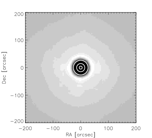
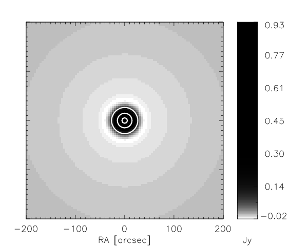
Fig. 2(a) shows the PSF that applies to the AzTEC map of Fig. 1. Strictly speaking, the PSF of Fig. 2(a) only applies to a point source at a particular location on the map. Therefore, before adopting assumption 1 of section II.2, we constructed several PSFs that apply to different locations on a map and verified that they are all very similar (at the few percent level) in terms of amplitude, width, and general shape [15]. The only noticeable difference between these PSFs is the orientation of the low-level asymmetric features seen in Fig 2(a). Therefore, we use a rotationally symmetrized version of the PSF, shown in Fig. 2(b), as the filter template. To evaluate the inaccuracy introduced by rotationally symmetrizing the PSF, we have fit the PSF of Fig. 2(b) to the PSF of Fig. 2(a), and find that the best fit amplitude differs from the actual amplitude of Fig. 2(a) by %, which is small compared to other errors we expect. Therefore, we adopt assumption 1 and the rotationally symmetrized PSF of Fig. 2(b).
Assumption 2 of section II.2 would be difficult to adopt if the field is imaged only once, so that the field has an essentially fixed Az-El orientation during the observation and each point on the map is scanned over in essentially one direction. However, AzTEC and other mm/sub-mm surveys routinely adopt assumption 2 because each of the mapped fields is imaged many times with varying orientations and scan directions. This is evident in Fig. 2(a) where the grey scale has been stretched to highlight the low-level asymmetric features of the PSF. We believe that such features are due to a small anisotropy in the final aggregate of scan directions from the 45 observation of this field. However, the fact that these features are so faint compared to the symmetric central parts (refer to the color bar of Fig. 2) supports our adoption of assumption 2.
V.2 Estimation of the PSD
In the AzTEC data analysis, the PSD corresponding to an observation is evaluated using Fourier transforms (FTs) of noise realization maps. Our noise realizations are generated using a “jackknife” method, where the signs of the detector time-streams are switched many times for each observation prior to map making [15]. An important consideration is to use long-enough time lags between the random sign switchings in order to preserve long-range noise features (low-frequency map noise) due to residual atmospheric contamination and instrumental drifts. The s time scales used are longer than the scan turn-around times but short enough that astronomical signal will not show up in noise realizations. Next, the noise realization time-streams are put through the same cleaning and filtering steps as the actual data, before maps are made. For a map such as Fig. 1, we generate 100 independent noise realization maps.
Because noise realizations are used for generating the PSD, it is free from astronomical signal and only includes the two dominant noise sources, residual atmospheric contamination and instrumental noise. The sub-dominant yet noticeable contribution of confusion noise is left out from the PSD for convenience.11 1 We note that other analyses that make use of the filtered signal map, such as estimating de-boosted source fluxes, stacking analyses, and number-counts estimates will not be skewed by the omission of confusion noise due to the use of source realizations and/or the AzTEC PSF having zero mean [15, see]. On the other hand, source lists for follow-up observations, which are based purely on will be very slightly biased due to the omission of confusion noise. This bias would favor peaks found in regions that have an over-density of unresolved sources, which can be beneficial to our understanding of SMGs and their environments. However, the method presented here, of using a PSD to characterize noise correlations, can fully accommodate astronomical “noise sources” such as confusion noise. For instance, Chapin et al. [9] describe how confusion noise was included in their matched filter. In general, astronomical effects such as confusion noise are frequency dependent. At longer wavelengths, a method for including the CMB within a matched filter is described in Tegmark & de Oliveira-Costa [18].

In our case, the noise PSD is generated by truncating each noise map to include only the central % coverage region (see Fig. 1(b)). Then, the 2-d FTs obtained from these regions are rotationally symmetrized and averaged to obtain the PSD shown in Fig. 3. As expected, the noise increases with decreasing over most of the range. A broad peak is visible at which is close to the FWHM of the PSF. This, we believe, is caused by the optical imaging of atmospheric fluctuations in between the random sign switches used to generate noise realizations. Near the scale, the PSD turns over and starts to decrease. This decline cannot be a map-size effect because the % coverage region used to construct the PSD extends in all directions. We believe that the PSD’s turn-over is real and that it is caused by the principle component analysis (PCA) based cleaning that the data is put through prior to map making, in order to mitigate the effects of atmospheric contamination and detector cross-talk. As PCA cleaning makes use of detector-detector time-stream correlations to “subtract” out these effects, it makes sense that the PSD shows a decline on the scale of the detector array (the spacing of individual detector beams is and the footprint of the entire array is for AzTEC-ASTE). To test if this long-range decline in the PSD is indeed real, we have performed the optimal filter presented here using the measured PSD as well as a modified PSD that plateaus at small as indicated by the dotted line of Fig. 3. The fact that there is no perceptible difference in results indicates that the map noise power is indeed low at low As noted earlier, an important property of the PSD of Fig. 3 is that it is a smoothly varying function, as opposed to a narrowly peaked one.
V.3 Filtering of maps
Once the PSF and PSD are available, the methods of section IV can be applied to obtain the filtered signal and coverage maps. In practice, more time is spent on the calculation of than the calculation of during the filtering process, even though involves a more complex calculation (see section IV). This is because needs to be evaluated separately for the actual map and each noise realization, as depends on (see Eq. 6), while needs to be evaluated only once for all 101 maps. For the example field used, the filtered signal and coverage maps are shown in Fig. 4.
 |
 |
| (a) | (b) |
The filtered coverage map must be filled with values and therefore, according to Eq. 10, it is simply equal to the map But is generated by propagating the initial noise variances, according to Eq. 7. Thus the noise estimates contained in are only as good as the starting noise estimates which are computed from estimates of individual detectors’ noise levels “near the time” that they contribute a sample to the map pixel in question [see 15, for details]. Therefore, before proceeding to the step of identifying point sources, we check the accuracy of noise estimates contained in using noise realization maps. First, we form a second noise estimate for each pixel by taking the standard deviation of the 100 noise-map values found at that pixel. Next, we form a second coverage map filled with the values Although provides a robust estimate of coverage, it is noisier than the the original coverage map due to the sample size of 100 (we expect a 7% error in for this sample size). Despite the noisy appearance of , its overall shape agrees very well with However, and often differ from each other by an overall scaling factor. We determine this scaling factor by comparing the average values of and in the 70% coverage region and applying a correction factor to in order to obtain the final filtered coverage map. Thus, the filtered coverage map is where
| (20) |
and usually lies in the range 0.85-0.95, depending on the field. Although we use just the 70% coverage region to find the agreement between and remains good out to the very edge of the mapped region until the coverage dips below 5%. Beyond this region, is consistently larger than Therefore, we do not trust the filtered coverage map beyond the 5% region and exclude this area when searching for point sources. Finally, in Fig. 5, we present the filtered signal-to-noise map, which is used directly to find point sources. It is generated by dividing the filtered signal map () by the filtered noise map ().22 2 The correction factor does not need to be applied in generating the filtered signal map because and both contain two factors of (see Eq. 6 and Eq. 7).

VI Results and discussion
It is encouraging that the signal-to-noise map of Fig. 5 has its most prominent peaks near the center, where the coverage is highest, and that the number of peaks as well as their amplitude declines smoothly toward the outer regions. Thus, even though the filtered signal map has large fluctuations near the edges (see Fig. 4(a)), the noise in those regions are accounted for in this optimal filter and there in no need for a by-hand coverage cut to eliminate spurious behavior near the edges. Throughout the AzTEC data analysis campaign, which has led to the publication of many source lists, variations of the filter presented here have been used. Therefore, the effectiveness of this technique may be assessed by the success rate of follow-up observations. In this regard, AzTEC has enjoyed an excellent record thus far. For instance, of 15 AzTEC point sources followed up by the Submillimeter Array (SMA), all were successfully observed [24, 25]. This is a very good record in comparison to the usual success rate of mm/sub-mm follow up studies.
In terms of weighting a fit according to all possible sources of uncertainty, the filtering technique presented in section IV (filter A) is clearly closer to optimal than the standard matched filter discussed in section III (filter B), especially in the presence of significant coverage gradients. However, filter A contains a larger number of steps and computations. In terms of implementation, we have shown that the intricacies of filter A have virtually no effect on the total computing time devoted to a field. However, converting these additional steps into functional computer code does require more time and effort. Therefore, it is fair to ask how much better filter A performs compared to filter B in a practical application. Of course, the answer depends on the specifics of the application. For instance, the acuteness of coverage gradients in a map will be important for this assessment. We will try to answer this question in the context of the typical AzTEC map that we have used here for illustrative purposes.
First, when a fit is closer to optimal, it yields smaller error bars on the fit parameters than a less optimized fit. A fair way of comparing error bars here is to compare the maps (generated using noise realizations, as described in section V.3) that result from the two filters. We find that the post-filter coverage () is on average 5-6% better with filter A than with filter B over most of the map, including the % coverage region. Thus, filter B is more prone to error, which in this context leads to higher rates of false detections as well as non-detections of truly significant sources.
| Map region | Filter A | Filter B | B but not A |
|---|---|---|---|
| 70% coverage | 31 | 31 | 2 |
| 30-70% coverage | 15 | 18 | 3 |
To form an impression regarding these rates, we summarize in table 1 the results obtained with each filter in different regions of the map. The “source candidates” reported in table 1 are defined to be peaks in the signal-to-noise map (Fig. 5) that exceed a value of 3.5. This is a good choice of threshold because, on average, pure noise realizations yield only noise peak with signal/noise over the entire map. Given the non-uniformity of coverage within the 30-70% region, it is not surprising that filter B “detects” 3 peaks that are judged by filter A (more accurately) to have It is interesting that even in the % coverage region, the source lists generated with filters A and B differ by two sources. The results reported in table 1 provide some grounds for the reader to gauge whether the additional work involved in implementing filter A is worth the effort. Of course, the optimal filter presented here will be most useful when the coverage of a field has large non-uniformities, unlike in the example field used here.
Thus far, many AzTEC publications only provide source lists from map regions with % coverage. As the optimal filter presented here is geared to handle coverage non-uniformities, we believe that the reliable region for source extraction can be extended to lower coverage thresholds. As mentioned in section V.3, regions with % coverage should be excluded. In fact, it may be best to exclude a larger region. For instance, not all elements of the detector array have imaged the outer regions of the map. Therefore, those regions may be systematically biased in some way compared to regions viewed and appraised by all detectors. Given that the AzTEC-ASTE detector array has a foot print on the order of it is reasonable to leave out a border of half that size, and use the % coverage region of Fig. 5 for source identification. This represents an increase of 75% in the source extraction area. Table 1 shows that % more source candidates can be obtained this way.
The optimal filter described here is now part of the AzTEC data
analysis pipeline, which may be downloaded (by anonymous ftp)
at
http://www.astro.umass.edu/aztec/Software/software.html. Within
this suite, the particular IDL routine that implements the optimal
filter
is aztec_adapative_wiener_filter.pro.
Appendix A Appendix: Fourier transform conventions
In this work, denotes the discrete 2-dimensional Fourier transform of the function Following the convention used by IDL and other high-level programing languages, this Fourier transform is defined as
| (A1) |
where and are the number of pixels in the and dimensions. Therefore, The and above, take on the and values of all the pixel centers. The and above assume integer values in the range and respectively. The discrete points on the reciprocal plane, where is defined are specified by
| (A2) | |||
| (A3) |
where is the pixel size. The corresponding inverse Fourier transform, denoted is defined as
| (A4) |
According to these conventions, the discrete convolution theorem takes on the form
| (A5) |
when and are real functions. In Eq. A5, is an index over all pixels of the map rather than a single dimension and similarly, is an index over all sampled points on the 2-d reciprocal plane.
References
- [1] Austermann, J. E. et al. 2010, MNRAS, 401, 160, 0907.1093
- [2] Barnard, V. E., Vielva, P., Pierce-Price, D. P. I., Blain, A. W., Barreiro, R. B., Richer, J. S., & Qualtrough, C. 2004, MNRAS, 352, 961, arXiv:astro-ph/0405156
- [3] Barreiro, R. B., Sanz, J. L., Herranz, D., & Martínez-González, E. 2003, MNRAS, 342, 119, arXiv:astro-ph/0302245
- [4] Baugh, C. M., Lacey, C. G., Frenk, C. S., Granato, G. L., Silva, L., Bressan, A., Benson, A. J., & Cole, S. 2005, MNRAS, 356, 1191, arXiv:astro-ph/0406069
- [5] Bertoldi, F., et al. 2007, ApJS, 172, 132
- [6] Béthermin, M. et al. 2012, ApJ, 757, L23, 1208.6512
- [7] Blain, A. W., Smail, I., Ivison, R. J., Kneib, J.-P., & Frayer, D. T. 2002, Phys. Rep., 369, 111, astro-ph/0202228
- [8] Borys, C., Chapman, S., Halpern, M., & Scott, D. 2003, MNRAS, 344, 385, arXiv:astro-ph/0305444
- [9] Chapin, E. L. et al. 2011, MNRAS, 411, 505, 1003.2647
- [10] Coppin, K., et al. 2006, MNRAS, 372, 1621, astro-ph/0609039
- [11] Downes, T. P., Welch, D., Scott, K. S., Austermann, J., Wilson, G. W., & Yun, M. S. 2012, MNRAS, 423, 529, 1103.3072
- [12] Ezawa, H. et al. 2008, SPIE Conf. Series, 7012, 6E
- [13] Humphrey, A. et al. 2011, MNRAS, 418, 74, 1107.3120
- [14] Perera, T. A. et al. 2008, MNRAS, 391, 1227, 0806.3791
- [15] Scott, K. S. et al. 2008, MNRAS, 385, 2225, 0801.2779
- [16] Scott, K. S. et al. 2012, MNRAS, 423, 575, 1203.2609
- [17] Stetson, P. B. 1987, PASP, 99, 191
- [18] Tegmark, M., & de Oliveira-Costa, A. 1998, ApJ, 500, L83, arXiv:astro-ph/9802123
- [19] Valiante, E., Lutz, D., Sturm, E., Genzel, R., & Chapin, E. L. 2009, ApJ, 701, 1814, 0906.4110
- [20] Vieira, J. D. et al. 2010, ApJ, 719, 763, 0912.2338
- [21] Vio, R., Andreani, P., & Wamsteker, W. 2004, A&A, 414, 17, arXiv:astro-ph/0305246
- [22] Weiß, A. et al. 2009, ApJ, 707, 1201, 0910.2821
- [23] Wilson, G. W. et al. 2008, MNRAS, 386, 807, 0801.2783
- [24] Younger, J. D. et al. 2007, ApJ, 671, 1531, 0708.1020
- [25] Younger, J. D. et al. 2009, ApJ, 704, 803, 0909.3299
- [26] Zeballos, M. et al. in prep., MNRAS