Anomalous radiative transitions between $h_{b}(nP)$ and $\eta_{b}(mS)$ and hadronic loop effect

Besides reporting the evidence of a bottomonium $\eta_{b}(2S)$, the Belle Collaboration recently measured several branching ratios of the radiative transitions between $h_{b}(nP)$ ($n=1,2$) and $\eta_{b}(mS)$ ($m=1,2$), i.e., $\mathcal{B}[h_{b}(1P)\to\eta_{b}(1S)\gamma]=(49.2\pm 5.7^{+5.6}_{-3.3})\%$, $\mathcal{B}[h_{b}(2P)\to\eta_{b}(1S)\gamma]=(22.3\pm 3.8^{+3.1}_{-3.3})\%$ and $\mathcal{B}[h_{b}(2P)\to\eta_{b}(2S)\gamma]=(47.5\pm 10.5^{+6.8}_{-7.7})\%$ [1]. As indicated in Ref. [1], there exists a discrepancy between these experimental values and theoretical expectations, where the branching ratios [1] measured are a factor of $1.2\sim 2.5$ higher than the corresponding theoretical results given in Ref. [2]. This anomalous radiative transition between $h_{b}(nP)$ and $\eta_{b}(mS)$ stimulates us to propose a solution to this problem.

In the past years, experimentalists have observed many anomalous hadronic decays and novel phenomena of higher charmonia and bottomonia, which include the excessive non-$D\bar{D}$ component of the inclusive $\psi(3770)$ [3, 4], the Okubo-Zweig-Iizuka (OZI) suppressed processes $\chi_{c1}\to\omega\omega,\phi\phi$ and double-OZI suppressed $\chi_{c1}\to\omega\phi$ [5], the $\chi_{cJ}$ radiative decays into a light vector meson [7, 6], the transitions of $\psi(4040)/\psi(4160)$ into $J/\psi\eta$ [8, 9, 10], and anomalous large rates of $e^{+}e^{-}\to\Upsilon(1S,2S)\pi^{+}\pi^{-}$ near the peak of the $\Upsilon(5S)$ resonance [11]. Explaining these phenomena, some theoretical efforts have been rewarded [12, 13, 14, 15, 16, 17, 18, 19], where the hadronic loop effects as an important QCD non-perturbative mechanism are introduced in these heavy quarkonium decays. Successfully explaining the observed experimental phenomena, we realize that the hadronic loop indeed plays a crucial role to the decays of heavy quarkonia.

In addition, some discrepancies also appear between experimental measurements and theoretical predictions on the radiative transition between charmonia. The experimental measurements for $J/\psi\to\eta_{c}\gamma$ and $\psi^{\prime}\to\eta_{c}/\eta_{c}^{\prime}\gamma$ [20] are much smaller than the nonrelativistic and relativistic Godrey-Isgur quark model predictions [2]. To alleviate the discrepancy between experimental measurements and naive quark model predictions, the meson loop contributions have been considered in Refs. [21, 22] and good agreements with the experimental measurements have been archived.

Along this line, in this work we adopt the hadronic loop effect to investigate the anomalous radiative transitions between $h_{b}(nP)$ and $\eta_{b}(mS)$ observed by the Belle Collaboration [1]. In this study, we first need to answer whether the discrepancy between the experimental and theoretical results of these radiative decays can be alleviated by including the hadronic loop contribution added to the tree level diagram. If this answer is affirmative, the hadronic loop effect, extensively applied to study intriguing higher charmonium and bottomonium decays recently observed, can be further tested, which will make our knowledge of non-perturbative QCD become abundant. In the next section, the details of the hadronic loop effects on $h_{b}(1P)\to\eta_{b}(1S)\gamma$, $h_{b}(2P)\to\eta_{b}(1S)\gamma$, and $h_{b}(2P)\to\eta_{b}(2S)\gamma$ will be explicitly presented. For the convenience of our presentation, these transitions are abbreviated as $h_{b}(nP)\to\eta_{b}(mS)\gamma$ in the following sections.

This paper is organized as follows. After the introduction, we illustrate the detailed formula of calculating the radiative transitions between $h_{b}(nP)$ and $\eta_{b}(mS)$. In Sec. III, the numerical results are given by comparing them with experimental data. The last section is devoted to a short summary.

In the naive quark model, the E1 transitions between $P$-wave and $S$-wave spin-singlets are written as [2]

where $\alpha$ is the fine-structure constant and $e_{Q}=-1/3$ denotes the charge of the bottom quark in units of $|e|$. $\omega$ is the energy carried by the emitted photon. The spatial matrix element $\langle{{}^{1}S_{0}}\left|r\right|{{}^{1}P_{1}}\rangle$ is relevant to the radial wave functions of initial and final heavy quarkonia.

In Fig. 1, we give the typical quark-level diagrams depicting $h_{b}(nP)\to\eta_{b}(mS)\gamma$ in the naive quark model. In the naive quark model, a loop diagram is usually ignored when calculating the $h_{b}(nP)\to\eta_{b}(mS)\gamma$ transition. As indicated by Belle [1], the measured branching ratio of $h_{b}(nP)\to\eta_{b}(mS)\gamma$ is not consistent with the result obtained in the naive quark model [2] which uses only Fig. 1 (a). Considering this situation, we need to introduce the higher order diagram shown in Fig. 1 (b), where $h_{b}(nP)$ first couples with two virtual bottom and anti-bottom mesons, which then turn into $\eta_{b}(mS)\gamma$ via exchanging bottom meson. However, it is rather difficult to calculate this kind of diagram Fig. 1 (b), so we would like to work in hadronic level diagrams. Here, we assume one to one correspondence between quark tree diagrams and meson tree diagrams as well as quark loop diagrams and meson loop diagrams. This is an assumption, but even now it is clear indirectly. It would be worthwhile to test it in future investigations when data will become more accurate.

The hadronic tree level contribution to the E1 transition corresponding to Eq. (1) is given as follows. Assuming a point form factor of electromagnetic interaction and considering the gauge invariance of the photon field, we can construct the Lorentz structure of the tree amplitude for the $h_{b}(nP)\to\eta_{b}(mS)\gamma$ process as

Here the effective coupling $g_{\text{QM}}$ can be extracted by comparing the decay widths, Eqs. (2) and (1). The sign of $g_{\text{QM}}$ is set to be positive in the present work. As indicated in the introduction, for $h_{b}(nP)\to\eta_{b}(mS)\gamma$ transitions there exists a discrepancy between the experimental measurement by Belle [1] and the predictions by the naive quark model [2].

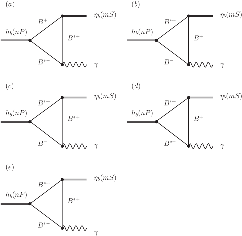
In the following, we introduce the meson loop contributions other than the tree contribution given by Eq. (2) when studying $h_{b}(nP)\to\eta_{b}(mS)\gamma$ decays. Then we would like to answer the question whether the discrepancy can be alleviated by the hadronic loop effect or not. To calculate the diagrams shown in Fig. 2, the effective Lagrangian approach is adopted, where we use the following Lagrangians constructed in heavy quark limit [23, 24, 25, 26, 27]:

where $\mathcal{B}_{\alpha\beta}^{\ast}=\partial_{\alpha}B_{\beta}^{\ast}-\partial_{\beta}B_{\alpha}^{\ast}$. In the heavy quark limit, the couplings among $h_{b}/\eta_{b}$ and the bottomed meson pair can be related to two gauge coupling constants $g_{1}$ and $g_{2}$ by

where $h_{b}(nP)$ and $\eta_{b}(mS)$ are abbreviated as $h_{b}$ and $\eta_{b}$, respectively. Thus, we need only to determine $g_{1}$ and $g_{2}$ corresponding to the couplings of $h_{b}(nP)$ and $\eta_{b}(mS)$, i.e., $g_{1}=-\sqrt{m_{\chi_{b0}(nP)}/3}/f_{\chi_{b0}(nP)}$ and $g_{2}=\sqrt{m_{\Upsilon(mS)}}/(2m_{B}f_{\Upsilon(mS)})$. The decay constants of $P$-wave bottomonium $f_{\chi_{b0}(1P)}$ and $f_{\chi_{b0}(2P)}$ can be related to the radial wave function of bottomonia [28], i.e., $f_{\chi_{b0}(1P)}=265$ MeV and $f_{\chi_{b0}(2P)}=282$ MeV. In addition, $f_{\Upsilon(1S)}=715$ MeV and $f_{\Upsilon(2S)}=482$ MeV are decay constants of $\Upsilon(1S)$ and $\Upsilon(2S)$, respectively, which are evaluated by their leptonic decay widths [29]. As for the $B^{\ast}B\gamma$ coupling constant, we adopt $g_{B^{\ast+}B^{+}\gamma}=1.311\,\mathrm{GeV}^{-1}$ and $g_{B^{\ast 0}B\gamma}=-0.749\,\mathrm{GeV}^{-1}$, both of which are estimated by the light-front quark model [30].

Having these effective Lagrangians, we obtain the decay amplitudes corresponding to the diagrams listed in Fig. 2 for the process $h_{b}(p_{0})\to[B^{(*)}(p_{1})B^{(*)}(p_{2})]B^{(*)}(q)\to\eta_{b}(p_{3})\gamma(p_{4})$, which read as

where the form factor $\mathcal{F}(q)$ is introduced to depict the internal structures and off-shell effects of the exchanged mesons as well as to remove the UV divergence in the loop integrals. In the present work, the form factor can be parameterized as [22]

with $q_{i}=q,p_{1},p_{2}$, where the parameter $\Lambda_{i}$ can be parametrized as $\Lambda_{i}=m_{i}+\alpha\Lambda_{QCD}$ with $m_{i}$ denoting the corresponding intermediate bottom meson mass and $\Lambda_{QCD}=220$ MeV. As illustrated in the caption of Fig. 2, there remain two more diagrams, whose amplitudes can be obtained by $\mathcal{M}_{c}$ and $\mathcal{M}_{d}$ by replacing the corresponding masses and the coupling constants.

In order to keep the gauge invariance of photon fields intact, the contact diagrams given in Fig. 3 should also be included in our calculation. The effective Lagrangian describing vertex of $\eta_{b}(mS)$ interacting with $B^{*}B^{(*)}\gamma$ is

where the coupling constants $g_{\eta_{b}B^{\ast}B\gamma}$ and $g_{\eta_{b}B^{\ast}B^{\ast}\gamma}$ can be obtained by the corresponding ones of $\mathcal{L}_{\eta_{b}B^{(\ast)}B^{(\ast)}}$, i.e., $g_{\eta_{b}B^{\ast}B\gamma}=e_{\bar{B}}g_{\eta_{b}B^{\ast}B}$ and $g_{\eta_{b}B^{\ast}B^{\ast}\gamma}=e_{B^{\ast}}g_{\eta_{b}B^{\ast}B^{\ast}}$ with $e_{\bar{B}}(e_{B^{\ast}})$ denoting the charge of $\bar{B}(B^{\ast})$ meson. By this effective Lagrangian, we obtain the amplitudes corresponding to the contact diagrams shown in Fig. 3, which are

In the above amplitudes, another form factor $\mathcal{F}_{\mathrm{Con}}(q^{2})$ should be introduced as a function of $q^{2}$, which cannot be arbitrary in order to keep the gauge invariance.

By summing over all decay amplitudes of the triangle hadronic loop diagrams and performing the loop integral, the general expression of amplitude for the triangle diagrams is parameterized as

On the other hand, the total amplitude of the contact diagram is

where the detailed deduction of the amplitudes for two contact diagrams is given in the Appendix.

With the above preparation, we finally get the total decay amplitude of $h_{b}(nP)\to\eta_{b}(mS)\gamma$ considering only the hadronic loop effect:

which must be gauge invariant. In Eq. (14), we define $f_{\text{ML}}=g_{\text{Tri}}+g_{\text{Con}}=f_{\text{Tri}}$, where $f_{\text{ML}}$ or $f_{\text{Tri}}$ is obtained by calculating these triangle diagrams shown in Fig. 2, which is our main task in this work.

As indicated above, in this work we will test whether including the hadronic loop contributions in $h_{b}(nP)\to\eta_{b}(mS)\gamma$ can alleviate a discrepancy between experimental and theoretical results. The total amplitudes for $h_{b}(nP)\to\eta_{b}(mS)\gamma$ transition is composed of $\mathcal{M}_{\text{QM}}$ given by Eq. (2) and $\mathcal{M}_{\text{ML}}$, i.e.,

where $\phi$ is the phase angle between the amplitudes due to different transition mechanisms. With these amplitudes, we can estimate the transition width as

where $m_{0}$ and $m_{3}$ denote the masses of $h_{b}(nP)$ and $\eta_{b}(mS)$, respectively.

Besides the coupling constants mentioned in Sec. II, the masses involved in our calculation are $m_{h_{b}(1P)}=9899.1$ MeV, $m_{h_{b}(2P)}=10259.8$ MeV, $m_{\eta_{b}(1S)}=9402.4$ MeV, and $m_{\eta_{b}(1S)}=9999.0$ MeV [1]. The properties of $P$ and $S$ wave singlet bottomonia are not well understood. At present, the full widths of $h_{b}(1P)$ and $h_{b}(2P)$ are still not yet measured by experiment. Thus, we have to adopt some theoretical estimation, since we need to apply these resonance parameters to obtain the experimental partial widths of $h_{b}(nP)\to\eta_{b}(mS)\gamma$, where the Belle Collaboration gave only the branching ratios of these decays [1]. Besides the radiative transition to lower bottomonia, $h_{b}(1P)$ and $h_{b}(2P)$ dominantly annihilate into three gluons ($ggg$) or two gluons plus one photon ($\gamma gg$). In Ref. [2], the widths of $h_{b}(1P)$ and $h_{b}(2P)$ decays into $ggg$ and $\gamma gg$ were given, i.e., $\Gamma(h_{b}(1P)\to ggg)=50.8$ keV, $\Gamma(h_{b}(1P)\to\gamma gg)=1.6$ keV, $\Gamma(h_{b}(2P)\to ggg)=50.2$ keV, and $\Gamma(h_{b}(2P)\to gg\gamma)=1.6$ keV. Thus we can obtain the branching ratio of $h_{b}(nP)\to\eta_{b}(mS)\gamma$, which is $\mathcal{B}[h_{b}(nP)\to\eta_{b}(mS)\gamma]=\Gamma_{h_{b}(nP)\to\eta_{b}(mS)\gamma}/\Gamma^{\mathrm{Tot}}_{h_{b}(nP)}$, where $\Gamma^{\mathrm{Tot}}_{h_{b}(nP)}=\sum_{m}\Gamma_{h_{b}(nP)\to\eta_{b}(mS)\gamma}+\Gamma_{h_{b}(nP)\to ggg}+\Gamma_{h_{b}(nP)\to\gamma gg}$. With the partial decay widths of $h_{b}(nP)\to ggg/\gamma gg$ from Ref. [2], we can roughly obtain the partial decay widths of $h_{b}(1P)\to\eta_{b}(1S)\gamma$, $h_{b}(2P)\to\eta_{b}(1S)\gamma$ and $h_{b}(1P)\to\eta_{b}(2S)\gamma$ as $38.9\sim 70.0$ keV, $18.9\sim 123.1$ keV, and $38.1\sim 267.9$ keV, respectively.

The lack of experimental measurement of the decay width of $h_{n}(1P)$ and $h_{b}(2P)$ leads to large uncertainties to the partial decay width of $h_{b}(nP)\to\gamma\eta_{b}(mS)$. To compare the coherent partial decay width including the amplitudes of quark model and meson loop with those estimated from the branching ratio, we adopt a large parameter space, which is $1\sim 4$ for $\alpha$ and $0\sim 2\pi$ for phase angle $\phi$. The $\gamma$ transition widths between $h_{b}(nP)\,\{n=1,2\}$ and $\eta_{b}(mS)\,\{m=1,2\}$ are present in Table 1. The results from naive quark model are smaller than the lower limit of the experimental measurements, especially for $h_{b}(2P)$ radiative decay. The meson loop gives sizable contributions in the radiative decay of $h_{b}(1P)/h_{b}(2P)$, and varies with parameter $\alpha$. The discrepancies between experimental measurements and theoretical estimation in the naive quark model can be alleviated.

In Fig. 4, we show the decay widths of $h_{b}(1P)\to\eta_{b}(1S)\gamma$, $h_{b}(2P)\to\eta_{b}(1S)\gamma$, and $h_{b}(2P)\to\eta_{b}(2S)\gamma$ dependent on $\alpha$ in the definition of $\Lambda_{i}$ and a phase factor $\phi$. The upper and lower limits of the experimental measurements are also presented as solid curves. The parts sandwiched by the curves are the parameter spaces allowed by the experimental measurements. The comparison between our numerical and the experimental results indicates that the hadronic loop contributions to $h_{b}(nP)\to\eta_{b}(mS)\gamma$ indeed can alleviate the discrepancy as mentioned in Sec. I. Thus, anomalous radiative transitions between $h_{b}(nP)$ and $\eta_{b}(mS)$ can be understood by introducing these hadronic loop diagrams. In addition, we also notice that there exist common $\alpha$ and $\phi$ ranges where the theoretical values are consistent with the experimental data of $h_{b}(nP)\to\eta_{b}(mS)\gamma$ (see Fig. 4 for more details). This phenomenon also reflects the similarity existing in the $h_{b}(1P)\to\eta_{b}(1S)\gamma$, $h_{b}(2P)\to\eta_{b}(1S)\gamma$, and $h_{b}(2P)\to\eta_{b}(2S)\gamma$ decays.

At present, there exists a large experimental range for these discussed $h_{b}(nP)\to\eta_{b}(mS)\gamma$ transitions [1]. We expect that future experiments can give a more precise measurement, which will be useful to further constrain our parameter range.

Being stimulated by Belle’s observation of anomalous radiative transitions between $h_{b}(nP)$ and $\eta_{b}(mS)$, in this work we study $h_{b}(nP)\to\eta_{b}(mS)\gamma$ transitions by introducing the hadronic loop contributions. As shown in our numerical results, the hadronic loop contributions play an important role to get consistent results with the experimental data [1]. These phenomena also show that the hadronic loop effects can be a universal mechanism existing in the charmonium and botttomonium hadronic and radiative decays, since there have been some theoretical efforts [12, 13, 14, 15, 16, 17, 18, 19] in this direction.

With more and more accumulation of experimental data, some novel phenomena of the decays of higher charmonium and bottomonium have been revealed. If inclusion of the hadronic loops is a universal non-perturbative QCD effect, we believe that the hadronic loop mechanism should be further tested in the future by comparing the results with more experimental observations, which is an intriguing and fruitful research field.

This project is supported by the National Natural Science Foundation of China under Grants No. 11222547, No. 11175073, No. 11005129, and No. 11035006, the Ministry of Education of China (FANEDD under Grant No. 200924, SRFDP under Grant No. 20120211110002, NCET), the Fok Ying Tung Education Foundation (No. 131006), and the West Doctoral Project of Chinese Academy of Sciences.

References

• [1] R. Mizuk et al. [Belle Collaboration], Phys. Rev. Lett. 109, 232002 (2012) [arXiv:1205.6351 [hep-ex]].
• [2] S. Godfrey and J. L. Rosner, Phys. Rev. D 66, 014012 (2002) [hep-ph/0205255].
• [3] M. Ablikim, J. Z. Bai, Y. Ban, X. Cai, H. F. Chen, H. S. Chen, H. X. Chen and J. C. Chen et al., Phys. Rev. D 76, 122002 (2007).
• [4] M. Ablikim et al. [BES Collaboration], Phys. Lett. B 641, 145 (2006) [hep-ex/0605105].
• [5] M. Ablikim et al. [BESIII Collaboration], Phys. Rev. Lett. 107, 092001 (2011) [arXiv:1104.5068 [hep-ex]].
• [6] M. Ablikim et al. [BESIII Collaboration], Phys. Rev. D 83, 112005 (2011) [arXiv:1103.5564 [hep-ex]].
• [7] J. V. Bennett et al. [CLEO Collaboration], Phys. Rev. Lett. 101, 151801 (2008) [arXiv:0807.3718 [hep-ex]].
• [8] X. L. Wang et al. [Belle Collaboration], arXiv:1210.7550 [hep-ex].
• [9] T. E. Coan et al. [CLEO Collaboration], Phys. Rev. Lett. 96 (2006) 162003 [hep-ex/0602034].
• [10] M. Ablikim, et al. [The BESIII Collaboration], arXiv:1208.1857 [hep-ex].
• [11] K. F. Chen et al. [Belle Collaboration], Phys. Rev. Lett. 100, 112001 (2008) [arXiv:0710.2577 [hep-ex]].
• [12] X. Liu, B. Zhang and X. -Q. Li, Phys. Lett. B 675, 441 (2009) [arXiv:0902.0480 [hep-ph]].
• [13] Y. -J. Zhang, G. Li and Q. Zhao, Phys. Rev. Lett. 102, 172001 (2009) [arXiv:0902.1300 [hep-ph]].
• [14] D. -Y. Chen, J. He, X. -Q. Li and X. Liu, Phys. Rev. D 81, 074006 (2010) [arXiv:0912.4860 [hep-ph]].
• [15] X. -H. Liu and Q. Zhao, Phys. Rev. D 81, 014017 (2010) [arXiv:0912.1508 [hep-ph]].
• [16] D. -Y. Chen, Y. -B. Dong and X. Liu, Eur. Phys. J. C 70, 177 (2010) [arXiv:1005.0066 [hep-ph]].
• [17] D. -Y. Chen, X. Liu and T. Matsuki, Phys. Rev. D 87, 054006 (2013) [arXiv:1209.0064 [hep-ph]].
• [18] C. Meng and K. -T. Chao, Phys. Rev. D 77, 074003 (2008) [arXiv:0712.3595 [hep-ph]].
• [19] C. Meng and K. -T. Chao, Phys. Rev. D 78, 034022 (2008) [arXiv:0805.0143 [hep-ph]].
• [20] M. Ablikim et al. [BESIII Collaboration], Phys. Rev. Lett. 108, 222002 (2012) [arXiv:1111.0398 [hep-ex]].
• [21] G. Li and Q. Zhao, Phys. Lett. B 670, 55 (2008) [arXiv:0709.4639 [hep-ph]].
• [22] G. Li and Q. Zhao, Phys. Rev. D 84, 074005 (2011) [arXiv:1107.2037 [hep-ph]].
• [23] H. Y. Cheng, C. Y. Cheung, G. L. Lin, Y. C. Lin, T. M. Yan and H. L. Yu, Phys. Rev. D 47, 1030 (1993) [arXiv:hep-ph/9209262].
• [24] T. M. Yan, H. Y. Cheng, C. Y. Cheung, G. L. Lin, Y. C. Lin and H. L. Yu, Phys. Rev. D 46, 1148 (1992) [Erratum-ibid. D 55, 5851 (1997)].
• [25] M. B. Wise, Phys. Rev. D 45, R2188 (1992).
• [26] G. Burdman and J. F. Donoghue, Phys. Lett. B 280, 287 (1992).
• [27] R. Casalbuoni, A. Deandrea, N. Di Bartolomeo, R. Gatto, F. Feruglio and G. Nardulli, Phys. Rept. 281, 145 (1997) [arXiv:hep-ph/9605342].
• [28] J. P. Lansberg, T. N. Pham, Phys. Rev. D79 (2009) 094016. [arXiv:0903.1562 [hep-ph]].
• [29] J. Beringer et al. [Particle Data Group Collaboration], Phys. Rev. D 86, 010001 (2012).
• [30] H. -M. Choi, Phys. Rev. D 75 (2007) 073016 [hep-ph/0701263].