Statistical inference framework for source detection of contagion processes on arbitrary network structures
Abstract
In this paper we introduce a statistical inference framework for estimating the contagion source from a partially observed contagion spreading process on an arbitrary network structure. The framework is based on a maximum likelihood estimation of a partial epidemic realization and involves large scale simulation of contagion spreading processes from the set of potential source locations. We present a number of different likelihood estimators that are used to determine the conditional probabilities associated to observing partial epidemic realization with particular source location candidates. This statistical inference framework is also applicable for arbitrary compartment contagion spreading processes on networks. We compare estimation accuracy of these approaches in a number of computational experiments performed with the SIR (susceptible-infected-recovered), SI (susceptible-infected) and ISS (ignorant-spreading-stifler) contagion spreading models on synthetic and real-world complex networks.
The structure of vast majority of biological networks (biochemical, ecological), technological networks (internet, transportation, power grids), social networks and information networks (citation, WWW) can be represented by complex networks [16], [7], [3]. Epidemic or contagion processes are amongst the most prevalent type of dynamic processes of interest characteristic for these real-life complex networks and they include disease epidemics, computer virus spreading, information and rumor propagation [23]. Different mathematical frameworks have been used to study epidemic spreading. We can divide them into two major categories based upon assumptions they make: the homogeneous mixing framework and the heterogeneous mixing framework. The homogeneous mixing framework assumes that all individuals in a population have an equal probability of contact. This is a traditional mathematical framework [12], [10] in which differential equations are used to model epidemic dynamics. The heterogeneous mixing framework assumes that properties of contact interactions among individuals are defined via some underlying network structure. The small world network property [24] and the scale-free network property [2] [8] have a great impact on the outcome of an epidemic spreading. We can further divide the heterogeneous mixing framework by other assumptions: the bond percolation, the mean-field and the particle network frameworks. The bond percolation approach applies the percolation theory to describe epidemic processes on networks [14], [11]. The mean-field approach assumes that all nodes having the same degree with respect to an epidemic process are statistically equivalent [4], [17]. The particle network approach assumes that spreading process is characterized by particles which diffuse along edges on a transportation network and each node contains some non-negative integer number of particles (reaction-diffusion processes).
The main question we address in this work is: Is it possible to detect location of the initial source from partial information on the contagion spread over a network structure ? This research question is useful for many realistic scenarios in which we observe epidemic spread at certain temporal moment and would like to infer the source location (patient-zero). Our statistical inference framework is applicable for arbitrary compartment contagion spreading model on arbitrary network structure. We have based our main case study on the SIR (susceptible-infected-recovered) model but we have demonstrated the applicability of inference framework on other contagion processes like the SI (susceptible-infected) and the ISS (ignorant-spreading-stifler) model. The SIR model [12] is an adequate model for many contagious processes like disease modelling, virus propagation [20] or rumour propagation [15]. We base our inference study on rather general assumptions which can be relaxed: (i) that observed partial epidemic realization is defined by complete knowledge of infected and recovered nodes (ii) that probabilities for infection and recovery of the underlying epidemic process are known in advance, as is the time from the start of the epidemic. We empirically demonstrate inference performance of the framework on different types of networks and for different contagion properties. We also investigate the impact on the performance of the framework in case when the assumptions are relaxed i.e. not complete knowledge on network status and when contagion parameters and time are uncertain. Finally, we demonstrate generality of the approach through solving source detection problem for different compartment models (SIR, SI and ISS).
Recently, the problem of estimating the initial source has gained a lot of attention due to its importance and practical aspects. Under different assumption on network structures or spreading process different source estimators have been developed [21],[6],[25],[18],[13]. However, we have made a significant contribution in problems of source detection for more general spreading processes on arbitrary network structures. In this work we cast this problem into a statistical inference framework based on the maximum likelihood estimation of the source of observed epidemic realization. This inference framework relies on a large scale simulation of contagion spreading processes from the set of potential source locations and subgraph similarity measures.
In section 1 we describe the SIR compartment model. Section 2 we describe our statistical inference framework and define different maximum likelihood estimators and subgraph similarity measures used to infer conditional probability of epidemic realizations from particular source locations. In section 3 we describe experiments that demonstrate network, contagion dynamics and noise effects and section 4 explains the related work.
Notation
| Notation | Description |
|---|---|
| is a network with a set of nodes and a set of edges | |
| general variable which identifies source nodes | |
| specific value for variable, example: the source node is the node | |
| probability of infection in one discrete time step | |
| probability of recovery in one discrete time step | |
| number of simulations for a specific SIR process | |
| temporal threshold (random variable or constant) | |
| epidemic random vector | |
| Bernoulli indicator random variable for node | |
| epidemic realization, example | |
| observed epidemic realization | |
| i-th component of the realization vector , example , | |
| random vector for realizations from node | |
| i-th sample realization vector from random vector | |
| set of potential sources | |
| similarity measure between two realizations | |
| random variable which measures the similarity between | |
| realization and realizations from random vector | |
| a bitwise XNOR function | |
| a bitwise OR function | |
| a bitwise AND function | |
| the similarity calculated with function | |
| the similarity calculated with function | |
| the Dirac delta function |
1 SIR compartment model
We define the contact-network as an undirected and non-weighted graph (-set of nodes or vertices, -set of links). A link exists only if two nodes and are in contact during the epidemic time. We also assume that the contact-network during the epidemic process is a static one. To simulate epidemic propagation through a contact-network, we use the standard stochastic SIR model. In this model each node at some time can be in one of the following states: susceptible (S), infected (I) and recovered (R). The spreading process is simulated using discrete time step model.
The SIR epidemic process is a stochastic process, which is simulated with mutually independent simulation steps on the contact network . At the beginning of each epidemic simulation all nodes from graph are in the susceptible state except set of nodes which are initially infected. We assume in our treatment that epidemic parameters and are predefined, constant and known beforehand. The epidemic parameter is the probability that an infected node infects an adjacent susceptible node in one discrete time step. The epidemic parameter is the probability that an infected node recovers in one discrete time step. Set of initially infected nodes is denoted with the letter . At the end of one full epidemic simulation, all nodes can be in one of two following states: susceptible or recovered. In our treatment however, we will limit epidemic spreading to a predefined number of discrete time steps, which basically means that we will deal with partially realized epidemic spreads and that this number of steps is also known parameter in the inference procedure for the source location estimation.
2 Statistical inference on epidemic propagation realizations
In this section we formulate the problem of the source localization in the network and develop related statistical inference framework.
Epidemic source location problem
Let us define the random vector , that indicates which nodes got infected prior up to some predefined temporal threshold (random variable or constant).
The random variable is a Bernoulli random variable, which assigns the value if node got infected before time from the start of the epidemic process and the value otherwise.
Let us assume that we have observed one spatio-temporal epidemic propagation realization of SIR process defined by and , and we want to infer which nodes from the set are the most likely source of realization for the SIR process and . is the finite set of possible source nodes that is defined by observed infected or infected and recovered set of nodes prior to moment in the network.
In order to find a node or a small subset of infected nodes that have highest likelihood for being the source of the epidemic spread, we pose the following maximum likelihood problem.
where is a set of all possible sources of epidemic.
By applying Bayes theorem, we get the following expression:
If all (apriori) are equally likely, this is equivalent to:
Thus, the core of source location estimation problem is the determination of the likelihood of the observed epidemic realization being initiated at the source location . We now proceed with description of the algorithms for determining the maximum likelihood for the observed epidemic realization.
2.1 The Maximum Likelihood source estimator
First, we give a pseudo-code (Algorithm 1) for the original problem of the maximum likelihood source estimation, where source can be any node from set . In principle, this treatment can be extended to problem of multiple sources determination, but the necessary extensions are out of the scope of this work. Note that among algorithm parameters the parameter represents number of random simulations from a single candidate for the epidemic source node. In our framework, the number of random simulations is very important from the perspective of the accuracy/stability of results and it is also a major determinant of the running time of the estimation procedure.
It is obvious that the Algorithm 1 is just a wrapper code that calls likelihood estimation function for each potential source of epidemics. We now proceed with the description of different algorithms for calculating the likelihood .
2.2 Realization similarity matching
Let us define the function , which measures the similarity between two epidemic realizations or subgraphs of the underlying network: and .
We first define new random variable , which measures the similarity between the fixed realization and random realization that comes from process with the source . We can calculate the unbiased estimator of the following cumulative distribution function as the empirical distribution function:
where is a characteristic function defined as:
Then, its probability density function is calculated like this:
where is the Dirac delta function.
Central limit theorem states that pointwise, has asymptotically normal distribution. The rate at which this convergence happens is bounded
by Berry–Esseen theorem. This implies that the rate of convergence is bounded by , where n is the number of random simulations.
Next, we define two measures ( and Jaccard) that are used to determine the similarity . The first one is a binary NOT XOR function or counts the number of corresponding non-infected and infected nodes in realizations and :
,where function is defined as:
In other words, is equal to one only if two nodes were infected or they did not get infected prior to temporal threshold . We also define function: , which is normalized function over total number of nodes: .
The second similarity measure is a well known Jaccard measure, which in our case counts the number of corresponding infected nodes in and in normalized by the number of corresponding infected nodes in or in .
where and functions are defined as:
and where function is defined as:
In the following text the will denote the similarity calculated with function and will denote the similarity calculated with function. In order to speed the similarity matching between realizations, we use the bitwise operations (XOR, NOT, AND) and bit count with Biran-Kernignan method.
2.3 Likelihood estimation functions
In this section we define three variants of likelihood estimation functions: AUCDF, AvgTopK, and Naive Bayes. First two functions, AUCDF and AvgTopK can use any of the similarity measures defined above, while Naive Bayes produces likelihood based on its own similarity measure.
As a first likelihood estimation function we define AUCDF (Area Under Cumulative Distribution Function) (see Algorithm 2), which can use any of the similarity measures defined above.
Different sources produce different empirical cumulative distributions of similarities to . If we compare two empirical distribution functions and from two different sources and and if the then sample of realizations from source are more similar to fixed realization than the sample realizations from source. This is the primary reason, why we use value to estimate source likelihood .
Algorithm AvgTopK represents a variant of the previous estimation function, which uses only highest values from the tail of the probability density function of the random variable :
In each simulation we calculate how similar realization to observed realization is by using function. Estimate is the average score over top highest similarities in simulations (tail of pdf).
Finally, we propose the third likelihood estimation function which is based on node probabilities for being infected from a particular source node. Main assumption of this approach is independence between nodes with respect to epidemic spreading.
The conditional probability that the node in realization is infected from source is:
where is the number of times that node got infected from the total of simulations from source node and is a smoothing factor. Smoothing factor is necessary to mitigate the problem of zero values, stemming from the finite number of simulations used to calculate .
Then we define the estimator for the likelihood of observing realization from source node as:
This equation uses the probability estimates that nodes from realization got infected and the probability estimates that nodes from realization did not get infected from source node .
In mathematical sense, probability of finding an infected node at time is dependent on other infected nodes prior to time . Nevertheless, we use the same assumption of independence to estimate the rank of potential sources. There is obvious resemblance between this approach and the well known studied probabilistic classifier - Naive Bayes. Although Naive Bayes uses a strong assumption of independence, it has been shown that in practice its performance is comparable to more complex probabilistic classifiers [9].
In order to have more stable numerical likelihood estimations, we used the log likelihood variant for estimating (see Algorithm 3).
3 Epidemic source location experiments
In this section, we describe the experiments along with the obtained results performed on different networks and in different epidemic settings. The experiments were designed to illustrate the overall predictability properties of the source detection problem with the introduced inference framework and compare the performances of individual algorithms.
We test the performance of source likelihood estimation algorithms on single source epidemic detection problems. In our experiments we observe one spatio-temporal epidemic propagation realization and we want to infer the potential source of realization from the set . In Figure 1, we illustrate one epidemic realization on a synthetic grid, where the color gradient from blue to red represents estimated source likelihood (blue - lower and red - higher ). We have used a Naive SIR algorithm implementation [1] as efficient SIR process simulation on network structures.

Due to the strong stochastic nature of epidemic process, frequency of correct estimations of the source location in the network is not the best measure to test the predictability of algorithms. The topological distance of maximum likelihood node from true source can be a misleading low even for random estimations on networks with low average shortest path. Therefore, we measure the rank of true source in the output list of potential sources from set in experiments on different network structures. The overall testing procedure is given in the following pseudo-code.
Let us assume that in some source location detection experiment we get realization that has infected nodes. We rank the nodes in a list of potential nodes according to the likelihood . We express the rank of real source as a relative source rank, i.e. the rank of the true source node normalized to the list size (for example, if the rank of the true source node is at the position in the list of potential sources, then the relative source rank is ). For the performed batch of experiments, we calculate cumulative source rank probability distribution, which tells us the probability that the relative rank of the source node is lower or equal to some specified value. By its nature cumulative source rank is very similar to the well known receiver operating characteristic (ROC), a measure frequently used in signal detection and machine learning for measuring the performance of classifier systems. Ideal estimator or classifier would have area under the cumulative source rank equal to one, exactly as in the case of ROC measure (AUC measure represents the area under the ROC curve). One can argue that other measures might have been appropriate as well, for example the distance of the maximum likelihood node to the true source node in a network. We opted for cumulative source rank, because it is a more versatile measure, due to its invariance to network size size and structure (e.g. for networks with different average shortest paths one would get grossly different results).
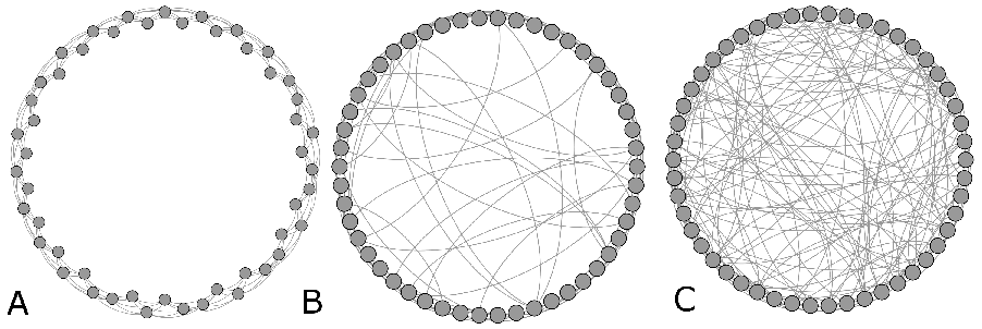
The influence of network structure on source localization performance has been tested on the following classes of networks: regular grid (figure 2) and lattice (figure 8 part A), Small-World networks (figure 8 part B), Erdös-Rényi networks (figure 8 part C), Albert-Barabasi network (figure 3 part A) and Western States Power Grid of the United States [24] (figure 3 part B).
In order to measure the performance of source localization we have done the following experiments:
- 1.
Comparison of different estimators: we compare performance of different algorithms for different epidemic conditions,
- 2.
Network structure experiments: this set of experiments illustrates the effects of network structure on the prediction performance over diverse network topologies,
- 3.
Process dynamics experiments: here we observe the effects of different process parameters like on source localization performance and
- 4.
Uncertainty experiments: Performance degradation associated with uncertain epidemic parameters or incomplete knowledge about epidemic realization.


Comparison of different estimators
In Figures 4,5 we can see the results of the source location detection experiment for different likelihood estimation functions (AUCDF, AvgTopK and Naive Bayes) on different network structures. The cumulative probability function in these experiments measure the probability of ranking the true source at specific position. These results suggest that Naive Bayes and AvgTopK estimators have better performance than the AUCDF estimator. For instance, we can see that in Figure 5 the Naive Bayes estimator ranks the true source in approximately 80 % of experiments in top 10 % of the source list. We have also made a baseline solution which uses random likelihood estimation function to rank the potential sources (see Figures 4,5). Random likelihood estimation function returns random uniform probability value for each node. Note, that the AvgTopK likelihood estimation function tends to give more accurate source localization performance than the Naive Bayes and AUCDF estimation functions. In our experiments we have used the top of highest scores from pdf in AvgTopK likelihood estimation function.


Network structure experiments
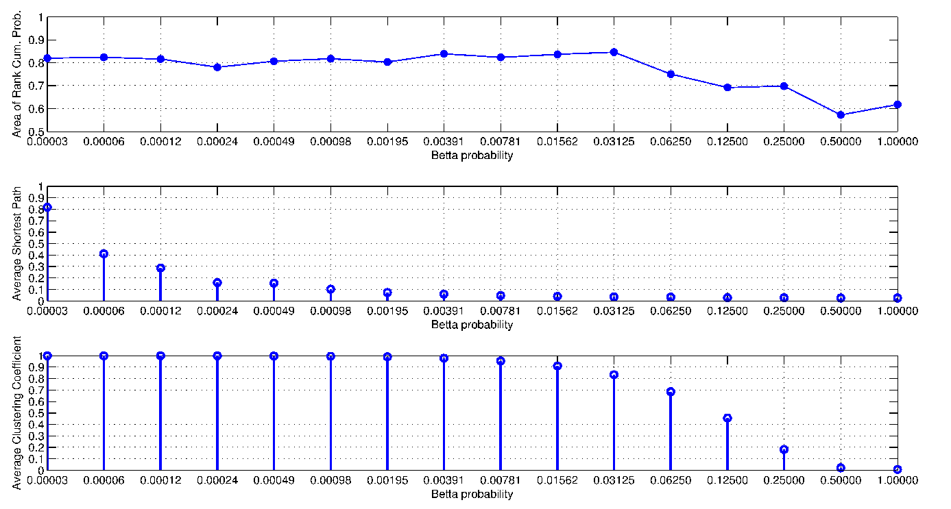
The effects of different network structures on source estimation performance is demonstrated with the following Small-World experiment. We are generating networks from regular lattice () to random networks () with Small-world networks in the middle and observing the performance of source estimators. We measure the area under the cumulative source rank function and observe that the performance of source estimator drops as the average shortest path of network decreases.
Process dynamics experiments
Finally, we perform a set of experiments to put our source location inference framework into a perspective with recent models for diffusion-like processes published in the literature [21] [18]. We illustrate performance of our inference framework on diffusion like processes which can be understood as a limiting case of SIR process in which recovery parameter is close to or equal zero. In Figure 9 and 10 we can observe that the performance of source estimation algorithms is highest in these conditions. This is expected behaviour which can be interpreted as a consequence of that initial conditions are preserved more in diffusion-like processes.


Uncertainty experiments
Note that the previous experiments were performed on processes for which the parameters , and were degenerative random variable i.e. constants. Now, we demonstrate the effects on performance when the exact values of , and are sampled from probability distributions. We model the temporal threshold as a random variable of the following form: , where represents the noise from some probability distribution. In Figure 11 we have made a series of experiments where the noise was modelled with the Geometric distribution with different parameters. As the variance of noise is increased, the performance of source localization is decreased. We have also made a series of experiments in which the parameters were also modelled with the noise: , , where noise was distributed as a Normal distribution with parameters . In Figure 12, we observe that the performance of source location decreases as the noise of parameters , and increases.
This findings suggest that if the predictability is low for parameters , and with no noise then predictability can only be lower when the noise is present.
Furthermore, this implies certain limits of predictability for source localization on Small-World networks.


In order to demonstrate the applicability of statistical inference framework for general type of compartment contagion processes, we have made a localization experiments with the information/rumor spreading ISS (ignorant-spreading-stifler) model. The ISS model divide the individuals to three groups: ignorants who have not heard the information/rumor, spreaders who are propagating the information/rumor to ignorants and stiflers who know the information/rumor and are no longer propagating it. The probability of spreading the information/rumor from spreaders to ignorants is in one discrete time step. If the spreader interacts with other spreader or stifler it turns to stifler state with probability of . The infected nodes in the SIR model recovery according to its internal state contrary to the ISS model where spreaders becomes stiflers according to states of its neighbours. In figure 13 we can observe the localization performance of inference framework on ISS model on regular grid for different parameters . Even in case when a fraction of random nodes in a network can be observed the statistical inference framework can localize the initial source (see figure 13).

4 Related work
Although the research of epidemic processes on complex networks is very mature the problem of epidemic source detection was formulated very recently. Various researchers have proposed different solutions to the problem of epidemic source detection which are based on number of assumptions on contact network structures and spreading models.
Zaman et. al. formulated a problem, where the rumor spreads with the SI model over network structure for some unknown amount of time and observe information about which nodes got infected. They rise a question who is the most likely source of the rumor and when can they find him. As a solution to the problem of source detection, they developed a rumor centrality measure, which is the maximum likelihood estimator for a regular trees under the SI model. They also obtained various theoretical results about the detection probability on different classes of trees [21],[22]. But, when the rumor spreading happens at the general graphs they use the simple heuristics that the rumour spreads along the breadth first search rooted at the source. Dong et. al. also studied the problem of rooting the rumor source with the SI model and demonstrate similar results of asymptotic source detection probability on regular tree-type networks [6].
Comin et. al. studied and compared different measures like degree, betweenness, closeness and eigenvector centrality as estimators for source detection [5]. Pinto et. al. also formulated a similar problem of locating the source of diffusion in networks from sparsely places observers [18]. They also assume that the diffusion tree is a breadth first search, the model of spreading with no recovery and the exact direction and times of infection transfers. Spectral algorithms for detection of initial seed of nodes that best explain given snapshot under the SI model has also been derived [19].
Zhu et. al. adopted the SIR model and proposed a sample path counting approach for source detection [25]. They prove that the source node on infinite trees minimizes the maximum distance to the infected nodes. They assume that the infected and susceptible nodes are indistinguishable. Lokhov et. al. use a dynamic message-passing algorithm to estimate the probability that a given node produces an observed snapshot. They use a mean-field-like approximation to compute the marginal probabilities and an assumption of sparse contact network [13].
Contrary to these approaches, our source estimation approach reduces the assumptions on network structures and spreading process properties. Our statistical inference framework can also work on arbitrary network structures and with arbitrary compartment spreading processes (SI, SIR, SEIR, ISS, etc.)
5 Conclusion
In this paper we have constructed a statistical framework for detecting the source location of an epidemic or rumour spread from a single realization of a stochastic contagion model on an arbitrary network. Detecting the source of an epidemic or rumour spreading under a stochastic SIR discrete model, represents an extension of existing research methodologies, mainly focussed on diffusion-like processes. Furthermore, this statistical framework can be deployed for different kinds of stochastic compartment processes (ISS, SI, SIR, SEIR) on networks whose dynamical patterns can be described by probability distributions over similarities among realization vectors. We have also demonstrated that we can relax even the assumptions on complete knowledge about epidemic realization, contagion process parameters and time with uncertainty.
Acknowledgements
The authors would like to thank Professor Yaneer Bar-Yam (New England Complex System Institute, Cambridge, MA 02142, USA) for valuable help in the early stages of the research.
References
- [1] N. Antulov-Fantulin, A. Lancic, H. Stefancic, M. Sikic, Fastsir algorithm: A fast algorithm for the simulation of the epidemic spread in large networks by using the susceptible-infected-recovered compartment model, http://arxiv.org/abs/1202.1639, Information Sciences (2013).
- [2] A.L. Barabasi, R. Albert, Emergence of scaling in random networks, Science 286 (1999) 509–512.
- [3] S. Boccaletti, V. Latora, Y. Moreno, M. Chavez, D.U. Hwang, Complex networks : Structure and dynamics, Phys. Rep. 424 (2006) 175–308.
- [4] C. Castellano, R. Pastor-Satorras, Thresholds for epidemic spreading in networks., Phys Rev Lett 105 (2010) 218701.
- [5] C.H. Comin, L. da Fontoura Costa, Identifying the starting point of a spreading process in complex networks, Phys. Rev. E 84 (2011) 056105.
- [6] W. Dong, W. Zhang, C.W. Tan, Rooting out the rumor culprit from suspects, http://arxiv.org/abs/1301.6312 (2013).
- [7] S.N. Dorogovtsev, A.V. Goltsev, J.F.F. Mendes, Critical phenomena in complex networks, Reviews of Modern Physics 80 (2008) 1275–1335.
- [8] S.N. Dorogovtsev, J.F.F. Mendes, A.N. Samukhin, Structure of growing networks with preferential linking, Phys. Rev. Lett. 85 (2000) 4633–4636.
- [9] D.J. Hand, K. Yu, Idiot’s Bayes—Not So Stupid After All?, International Statistical Review 69 (2001) 385–398.
- [10] H.W. Hethcote, The mathematics of infectious diseases, SIAM Review 42 (2000) 599–653.
- [11] E. Kenah, J.M. Robins, Second look at the spread of epidemics on networks, Phys. Rev. E 76 (2007) 036113.
- [12] W.O. Kermack, A.G. McKendrick, Contributions to the mathematical theory of epidemics, Proc. Roy. Soc. London Ser. A 115 (1927) 700–721.
- [13] A.Y. Lokhov, M. Mézard, H. Ohta, L. Zdeborová, Inferring the origin of an epidemy with dynamic message-passing algorithm (2013).
- [14] D. Mollison, Spatial contact models for ecological and epidemic spread, Journal of the Royal Statistical Society. Series B (Methodological) 39 (1977) 283–326.
- [15] Y. Moreno, M. Nekovee, A.F. Pacheco, Dynamics of rumor spreading in complex networks, Phys. Rev. E 69 (2004) 066130.
- [16] M.E.J. Newman, The Structure and Function of Complex Networks, SIAM Review 45 (2003) 167–256.
- [17] R. Pastor-Satorras, A. Vespignani, Epidemic spreading in scale-free networks, Phys. Rev. Lett. 86 (2001) 3200–3203.
- [18] P.C. Pinto, P. Thiran, M. Vetterli, Locating the Source of Diffusion in Large-Scale Networks, Physical Review Letters 109 (2012) 068702+.
- [19] B.A. Prakash, J. Vreeken, C. Faloutsos, in: ICDM’2012; Proceedings of the IEEE International Conference on Data Mining (2012).
- [20] G. Serazzi, S. Zanero, Computer virus propagation models, in: M. Calzarossa, E. Gelenbe (Eds.), Performance Tools and Applications to Networked Systems, volume 2965 of Lecture Notes in Computer Science, Springer Berlin Heidelberg, 2004, pp. 26–50.
- [21] D. Shah, T. Zaman, Detecting sources of computer viruses in networks: theory and experiment, in: Proceedings of the ACM SIGMETRICS international conference on Measurement and modeling of computer systems, SIGMETRICS ’10, ACM, New York, NY, USA, 2010, pp. 203–214.
- [22] D. Shah, T. Zaman, Rumors in a Network: Who’s the Culprit?, volume 57 of IEEE Transactions on Information Theory, pp. 5163–5181.
- [23] A. Vespignani, Modelling dynamical processes in complex socio-technical systems, Nat Phys 8 (2012) 32–39.
- [24] D. Watts, S. Strogatz, Collective dynamics of ’small-world’ networks, Nature 393 (1998) 440–442.
- [25] K. Zhu, L. Ying, Information source detection in the sir model: A sample path based approach, http://arxiv.org/abs/1206.5421 (2013).