On the Scission Point Configuration of Fisioning Nuclei
Abstract
The scission of a nucleus into two fragments is at present the least understood part of the fission process, though the most important for the formation of the observables. To investigate the potential energy landscape at the largest possible deformations, i.e. at the scission point (line, hypersurface), the Strutinsky’s optimal shape approach is applied.
For the accurate description of the mass-asymmetric nuclear shape at the scission point, it turned out necessary to construct an interpolation between the two sets of constraints for the elongation and mass asymmetry which are applied successfully at small deformations (quadrupole and octupole moments) and for separated fragments (the distance between the centers of mass and the difference of fragments masses). In addition, a constraint on the neck radius was added, what makes it possible to introduce the so called super-short and super-long shapes at the scission point and to consider the contributions to the observable data from different fission modes. The calculated results for the mass distribution of the fission fragment and the Coulomb repulsion energy ”immediately after scission” are in a reasonable agreement with experimental data.
Keywords:
nuclear fission, deformation energy, scission point, super-long, super-short shapes, mass distribution, total kinetic energypacs
02.60.Lj, 02.70.Bf, 21.60.-n, 21.60.Ev, 25.85.EcI Introduction
The shape of a nuclear surface is a basic notion in many theoretical models of nuclear structure and reactions. A good choice of the shape degrees of freedom reduces substantially the computation time and is often, especially for the description of fission process or fusion-fission reactions, a key to the success of the theory.
In past a lot of shape parameterizations were proposed and used. One class of shapes relies on the expansion in a complete set of functions like the expansion of the radius vector [1] or the profile function squared [2] in Legendre polynomials. In the parametrization [3] the deviation of the shape from the basic Cassini ovals is also expanded in Legendre polynomials. Another possibility is given by the introduction of a restricted number of deformation parameters, like in the parametrization of three smoothly joined quadratic surfaces [4], the two center shell model [5], the Funny-Hills parametrization [6] or modified Funny-Hills parametrization [7].
All these shape parametrizations are restricted to a certain class of shapes. In all these cases the question arises whether the given class of shapes is complete enough to represent the essential properties of the investigated process.
A method to introduce the shape of the nuclear surface which does not rely on any shape parametrization was suggested by V.Strutinsky already in [8, 9]. In this method one defines the profile function of an axially symmetric nucleus by the minimization of the liquid drop energy with respect to the variation of under additional constraints which fix the volume and elongation of the drop. However, due to numerical difficulties this method was not widely used in the past.
Only recently [10] it turns out possibly to solve the variational problem of [8] in a very broad region of deformations ranging from a disk (even with a central depression) to two touching spheres. The fission barriers calculated by this method [11] were found to be in a reasonable agreement with the experimental results.
In the present work the potential energy landscape is investigated for larger deformations - at the scission point (line, hypersurface). The scission of a nucleus into two fragments is at present the least understood part of the fission process, though the most important for the formation of the observable data.
For the accurate description of the mass-asymmetric nuclear shape at the scission point it turned out necessary to construct an interpolation between the two sets of constraints for the elongation and mass asymmetry which are applied successfully at small deformations (quadrupole and octupole moments) and for separated fragments (the distance between centers of mass and the difference of fragments masses). In addition, a constraint on the neck radius was added, what makes it possible to introduce the so called super-short and super-long shapes at the scission point and consider the contributions to the observable data from different fission modes.
The paper is organized as follows. Section II is a short overview of the Strutinsky optimal shapes prescription. The mass-asymmetric shapes are introduced in Sect. III. The scission shape and the shape of separated fragments ”immediately after scission” are defined in Sect. IV-V. In Sect. VI the super-short and super-long shapes are introduced and the calculated Coulomb repulsion energy of the fragments ”immediately after scission” is compared with the experimental total kinetic energy of fission fragments of . Sect. VII contains a short summary.
II The optimal shapes of fissioning nuclei
The shape of an axially symmetric nucleus can be defined by rotation of some profile function around the -axis. It was suggested in [8] to define the profile function looking for the minimum of the liquid-drop energy, , under the constraint that the volume and the elongation are fixed,
| (1) |
with
| (2) |
In (1) and are the corresponding Lagrange multipliers. The elongation parameter was chosen by [8] to be the distance between the centers of mass of the left and right parts of the nucleus,

The minimization of with respect to the profile function leads to an integro-differential equation for
| (3) |
Here is the Coulomb potential at the nuclear surface, and is the fissility parameter of the liquid drop [12],
| (4) |
where is the surface tension coefficient. In (4) and everywhere below the index (0) refers to the spherical shape.
By solving Eq. (3) one obtains the profile function for given and ( is fixed by the volume conservation condition). The liquid drop deformation energy (in units of the surface energy for a spherical shape)
| (5) |
calculated for the shapes shown in Fig. 1, is presented in Fig. 2. In (5) , .

One can see from Fig. 2 that the elongation of the shapes shown in these figures is limited by some maximal value . Above this deformation mono-nuclear shapes do not exist. This critical deformation was interpreted in [8] as the scission point. Note that, at scission the neck radius is still rather large: the neck radius at the critical deformation is approximately equal to for a fissility parameter in the range
Another peculiarity of Fig. 2 is the upper branch of the deformation energy at large deformation. Along this branch the neck of the drop becomes smaller and smaller until the shape turns into two touching spheres. Both branches are solutions of Eq.(3). It turns out, that the upper branch of corresponds not to the minimum but to the maximum of the energy. Thus, it represents the ridge of the potential energy surface between the fission and fusion valleys.
III The mass-asymmetric shapes
The optimal shape approach of [8] can be generalized to mass-asymmetric shapes. For this aim one has to include into Eq.(1) one more constraint fixing the mass asymmetry of the drop,
| (6) |
The mass asymmetry is commonly defined by the difference of masses and to the left and right of some point ,
| (7) |
In case that the drop has a neck, coincides with the position of the neck, . By we mean here the point where has a minimum. For the pear-like shape the neck does not exist and could be defined in a different way, see [10]. In the present work we are interested in the scission point configuration for which the neck is well defined. Then the Euler-Lagrange equation for the variational problem (6) has the form
| (8) | |||||
Eq.(8) can be solved in the same way as Eq.(3). Some examples of the shapes at the scission point (maximal possible value of ) for few values of the mass asymmetry are shown in Fig. 3.

The advantage of the variational problem in the form (6) is that the constraints for the elongation and the mass asymmetry have a clear physical meaning. These are the distance between the centers of mass of right and left part of the drop and the mass asymmetry of the drop.
The disadvantage is that due to the simplicity of the restrictions on and , equation (8) contains some unphysical effects. Namely, because is a discontinuous function of , the second order derivative , defined by Eq.(8), and, consequently, the curvature of the surface, is discontinuous at , what should not take place for a liquid drop. Besides, for a pear-like shape the neck does not exists and it is not so clear how one could define in this case. Some possibility to define as the place of the largest curvature of the surface was suggested in [10].
Besides and one could try another popular pair of constraints which are often used in the constrained Hartee-Fock calculations, namely, the quadrupole and octupole moments,
| (9) |
The moments and can be defined independently of whether the neck exists or not. The use of quadrupole and octupole moments as constraints
| (10) |
leads to the following Euler-Lagrange equation
| (11) |
with
| (12) | |||
Eq.(11) can be solved in the same way as Eq.(8). The examples of the scission point shapes for few value of the mass asymmetry are shown in Fig. 4.

Comparing the shapes at the scission point calculated by Eq. (8) and Eqs. (11)-(12) for the same mass-asymmetry one can see that these two sets of shapes are rather different. The restrictions lead to scission shapes which are considerably ”shorter” as compared with the scission shapes defined with restrictions.
The comparison of the energies at the scission point is shown in Fig. 5. Due to the smaller Coulomb repulsion energy for more elongated shapes the scission point energy calculated with the profile function (8) is by MeV lower than that calculated with the profile function (11)-(12).
The expansion in multipole moments is an expansion in the complete set of orthogonal functions. At small deformation only few lower moments are important. At large deformation, especially at the scission point, one can not characterize the optimal shape of the surface by the quadrupole and octupole moments alone. Higher multipole moments should then also be taken into account.

The optimal shapes defined with constraints describe well the separated or touching drops. For the shape with a neck one should try to define a constraint which would be an interpolation between and constraints. Some hint how this can be achieved, one can get looking at the curvature of the surface calculated with both constraints. At each point of the surface one can define the local curvature ,
| (13) |
where and are the local principal radii of curvature. In the case of axially symmetric shapes the radii and can be expressed in terms of the profile function ,
| (14) |
Inserting (14) into (13) and solving this equation with respect to one gets the following relation between the profile function and the local curvature ,
| (15) |
Comparing Eq.(15) and Eq.(11) one sees that the expression in curly brackets in (8) or (11) is just twice the local curvature of the surface.
The left-right asymmetric part of the curvature proportional to and (the length of the drop along the -axes is equal to ) is shown in Fig. 6. The function which appears in Eq.(10) grows rapidly at the tips of the drop (at ). At the tips of the drop the surface of the heavy fragment becomes flat, the surface of the light fragment becomes very deformed (elongated). This is in contradiction with the expectation that due to Coulomb repulsion the distant parts of the drop should be close to spheroids.
The spherical shape has a constant curvature. I.e. for the distant part of the drop the constraint is more meaningful than . It is also clear that at small (in the neck region) the curvature should change smoothly between the asymptotic values on the very left and on the very right.

These requirements can be fulfilled if instead of one would introduce a smoothed Sign - function, say by the replacement
| (16) |
and use these smoothed quantities as the constraints for the elongation and mass asymmetry. In (16) we have introduced also a smoother - function which appears in the definition (2) of constraint.
IV The scission shapes
The replacement (16) contains an additional parameter - the smoothing width . In principle, one can consider it as an additional collective parameter which has to be taken into account in the dynamical calculations. In the quasi-static limit one could expect that the value of is close the curvature radius in the neck region.
Replacing in (11) the and by the smoothed quantities (16) one gets the following equation for
| (17) |
In Figs. 7, 8 we show the optimal shape at the scission point calculated with the constraint (16) for two very different values of , and . The first is approximately equal to the neck radius, the second - to the half-length of the drop in -direction at the scission point.

The Figs. 7, 8 are similar to Figs. 3, 4. The shapes calculated with are rather close the shapes calculated with constraints (in the limit the profile functions shown in Fig. 3 and Fig. 7 coincide). The energies calculated with and constraints are also very close to each another, see Fig. 5. With growing the scission shapes are getting shorter like those calculated with the constraints. However the tips of the shapes calculated with are more ”spherical” as compared with those calculated with constraints. The energies of the shapes calculated with are by MeV lower as compared with the ones calculated with constraints.
Taking into account the results shown in Fig. 5, the shapes calculated with seem more preferable as the scission shapes. Besides, the total kinetic energy of the fission fragments calculated with is in better agreement with the experimental data as compared with the one calculated for (see the Fig. 14 below). So, in calculations below the shapes shown in Fig. 7 will be used as the scission shapes.

The description of the fission process requires a solution of the dynamical problem. The potential energy surface is important, but only one ingredient of the dynamical description. The inertia, friction and diffusion tensors are also equally important. Still, having only the potential energy surface at ones disposal, one could try to estimate some observable of the fission process.
Keeping in mind that the fission process is slow one could assume that during the fission process the state of the fissioning nucleus is close to thermal equilibrium, i.e. in the quasistatic limit the points on the deformation energy surface are populated with the probability given by the Boltzman factor,
| (18) |
Here is the temperature, and is a constant which is not important for what follows.
Then, the normalized mass distribution of the fission fragments will be defined by the deformation energy at maximal deformation considered as a function of the mass asymmetry for each pair of fragments,
| (19) |
where is the liquid drop energy (5) plus the shell correction .
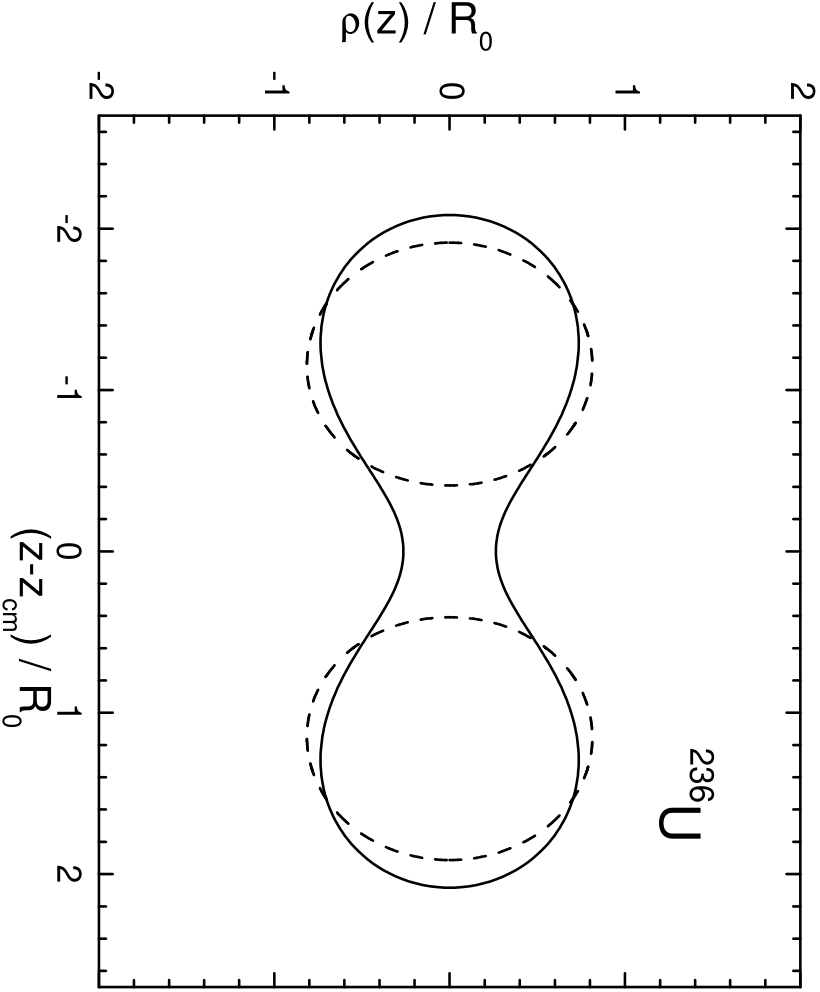
To calculate the shell correction energy we have approximated the shapes shown in Fig. 7 by the Cassini ovaloids with three deformation parameters , see [3], and for the shape given in terms of Cassini ovaloids calculated the single-particle energies and the shell correction by the code [3]. The liquid drop energy and the total energy including the shell correction for the nucleus are shown in Fig. 9.


The total energy has a minimum at the fragment mass equal to 95 or 141. Consequently the peaks of the mass distribution of the fission fragment are located at these fragments masses, see Fig. 9. The position of the peaks of the mass distribution is in good agreement with the well known experimental results [13]. This agreement can be considered as a confirmation that the scission point shape and energy are calculated correctly.
The distribution (18) is a basic assumption of the scission-point model suggested by [14] and developed further in [15, 16, 17], see also [18]. In this model the scision point configuration consists of two coaxial spheroids with tip-to-tip distance and quadrupole deformation parameters and . There are two temperatures in this model one for the population of the single-particle levels, , and one for the collective degrees of freedom, . The parameters , and were fitted in [14] in order to reproduce the experimental data. The was found to be close to 1 Mev. In the calculations shown in Fig. 10 we used the same value =1 MeV.
Note, that within the optimal shape approach the shape configuration is not fitted to the experimental results but is defined unambiguously from the minimal energy condition.
V The separated fragments
Within the optimal-shape method one can also find the optimal shape of separated fragments. For this aim one solves equation (3) with the initial conditions that correspond to two spherical fragments at large enough distance from each other. Making the distance smaller and smaller, one can find out how the shape of the fragments changes with the distance between their centers of mass.

The results of numerical calculations for the symmetric splitting of are shown in Fig. 11. The shape of the separated fragments is very close to oblate ellipsoids. The octupole deformation is very small. Its contribution to the deformation energy at the touching point of two nuclei is of the order 0.5 Mev only. The energy of separated fragments is shown by the dashed line in Fig. 12. The lower solid curve and the dashed line correspond respectively to the bottom of the fission and the fusion valleys and the upper solid curve to the ridge between the fusion and fission valleys.
The kinetic energy of the fission fragments is the kinetic energy gained by the fragments due to the Coulomb repulsion after separation plus the prescission kinetic energy. Within the quasi-static picture one can calculate only the energy of the Coulomb repulsion “immediately after scission”. At present it is not so clear how the scission process proceeds. For slow collective motion it is natural to assume that during the neck rupture the elongation (the distance between centers of mass of left and right parts of nucleus) does not change, like it is shown by arrow in Fig. 12. The corresponding profile functions at for the compact system and separated fragments are show in Fig. 13.

The Coulomb interaction energy of the fragments immediately after scission shown in Fig. 13 is easy to calculate. The only additional parameter (besides the fissility parameter ) which appears in such calculation is the parameter of the nuclear radius, . In the present work we used the value fm.
The comparison of the Coulomb interaction energy of the fragments immediately after scission with the experimental value of the total kinetic energy for the nucleus is shown in Fig. 14. The solid and dashed lines are calculated with (solid) and (dashed). One sees that the more elongated scission () shapes are in somewhat better agreements with the experimental data.
The agreement is of qualitative character only. For a more accurate description on should take into account the multimodal character of the fission of . The optimal shapes described above correspond to only one (standard) fission mode.

VI Super-long and super-short scission shapes
The optimal shapes discussed in Sections 3-5 have the two degrees of freedom - elongation and the mass asymmetry. The neck radius for the given elongation and the mass asymmetry attains the ”most favored” value which results from the minimum of the potential energy condition. In the dynamical calculations of the fission process the neck radius is often considered as an independent collective variable which can deviate from the one corresponding to the bottom of the potential energy surface. Thus, it makes sense to incorporate in the optimal shapes procedure the neck radius as another independent degree of freedom.
In order to include one additional degree of freedom in the optimal shapes procedure one should add another constraint fixing the neck radius. Usually, in various shape parameterizations, the neck radius is regulated by the parameter of the hexadecapole deformation. Using as an additional constraint, allows, indeed, to vary somewhat the neck radius of the drop. However, at large value of the constraint results in very peculiar shapes.
Another possibility to vary the neck radius is to fix the amount of matter in the neck region by introducing the constraining function of the type
| (20) |
For simplicity we assume here that has the same meaning and value as used in Sections 3-4.
The effect of on the optimal shapes is demonstrated in Fig. 15. Indeed, varying (keeping fixed) allows to change the neck of the drop in a rather broad region.

The introduction of the neck degree of freedom has an important consequence for the scission shape. Depending on the neck radius, the scission shapes become more elongated or shorter, see Fig. 16. Thus, it turns out possible to introduce the so called [22] super-long or super-short scission shapes which represent the possibility of the existence of few fission modes and are exploited by the interpretation of the experimental data, see for example [23].

The Coulomb interaction energy ”immediately after scission” for the super-long or super-short shapes shown in Fig. 16 is plotted in Fig. 14 by dash-dot and dash-dot-dot lines. Qualitatively these results are very close to the contribution from three fission modes [24] shown in Fig. 13 of [25]. For a more precise estimate of the contribution from the super-long or super-short scission shapes, full dynamical calculations (with the account of shell effects) are required.
VII Summary and Conclusions
The optimal-shape approach is put into practice by the construction of the constraint on the mass asymmetry which is an interpolation between the constraint on quadrupole and octupole moments (which is quite successful at small deformations) and the constraint on the distance between the centers of mass of the future fission fragments and the difference of their masses (which is well defined for the shape with a neck or separated fragments). The use of this new constraint allows to define the scission point shapes in broad region of the mass asymmetries.
It is shown that the optimal-shape procedure can be further extended by incorporating the neck degree of freedom. The introduction of the neck degree of freedom leads to the fission valleys, the existence of which follows from the analysis of experimental data.
The account of shell effects on the potential energy surface of the optimal drops will be the subject of future studies.
Acknowledgements
The author appreciates very much the fruitful discussions with Profs. J. Bartel, N. Carjan, H.-J. Krappe, V.V.Pashkevich, K. Pomorski and is grateful to the theory group of CENBG for the warm hospitality during his stay at Bordeaux.
References
- [1] S. Cohen, and W. J. Swiatecki, Ann. Phys. (N.Y.) 22, 406 (1963).
- [2] S. Trentalange, S. E.Koonin, and A. J. Sierk, Phys. Rev. C 22, 1159 (1980).
- [3] V. V. Pashkevich, Nucl. Phys. A 169, 275 (1971).
- [4] J. R. Nix, Nucl. Phys. A 130, 241 (1969).
- [5] J.Marhun and W.Greiner, Z.Physik 251, 431 (1972).
- [6] M. Brack, J. Damgaard, A. S. Jensen, H. C. Pauli, V. M. Strutinsky and C. Y. Wong, Rev. Mod. Phys. 44, 320 (1972).
- [7] K. Pomorski and J. Bartel, Int. J. Mod. Phys. E 15,417 (2006).
- [8] V. M. Strutinsky, N. Ya. Lyashchenko, N. A. Popov, Nucl. Phys.46, 659 (1963).
- [9] V. M. Strutinsky, Zh. Exp. Theor. Fiz. 45, 1891 (1963).
- [10] F. Ivanyuk, Int. J. Mod. Phys. E 18, 130 (2009).
- [11] F. Ivanyuk and K. Pomorski, Phys. Rev. C 79, 054327 (2009).
- [12] N. Bohr and J. A. Wheeler, Phys. Rev. 56, 426 (1939).
- [13] R. Vandenbosh and J.R. Huizenga, Nuclear Fission, Academic, New-York, 1973.
- [14] B. D. Wilkins, E. P. Steinberg, and R. R. Chasman, Phys. Rev. C 14, 1832 (1976).
- [15] J. Moreau, K. Heyde, and M. Waroquier, Phys. Rev. C 28, 1640 (1983).
- [16] A. Ruben, H. Marten, D. Seeliger, Zeit.für Physik A Hadrons and Nuclei 338, 67 (1991).
- [17] S. Panebianco, N. Dubray, H. Goutte, S. Heinrich, S. Hilaire, J.-F. Lemaitre, J.-L. Sida, The talk at the 3rd International Workshop on Nuclear Data Evaluation for Reactor Applications. Organised by CEA and NEA, WONDER 2012, Aix-en-Provence, 25-28 September 2012.
- [18] H.-J. Krappe and K. Pomorski, Theory of Nuclear Fission, Lecture Notes in Physics 838, Springer Verlag, Heidelberg, 2012.
- [19] R. Muller et al., Phys. Rev. C 29, 885 (1984).
- [20] H. Baba et al., J. Nucl. Sc. Techn. 34, 871 (1997).
- [21] S. Zeynalov et al., Proceedings of the XIII Seminar on Interaction of Neutrons with Nuclei, JINR-Dubna, p.351 (2006).
- [22] U. Brosa, S. Grossmann, A. Müller, Z. Naturfor. 41a, 1341 (1986).
- [23] F.-J. Hambsch, H.-H Knitter, C. Budtz-Jorgensen and J. Theobald, Nucl. Phys. A 491, 56 (1989).
- [24] F.-J. Hambsch, S. Oberstedt and I. Ruskov, private communication, 2012.
- [25] N. Carjan, F.A. Ivanyuk and V.V. Pashkevich, Physics Procedia 31, 66 (2012).