Synchronization of Weakly Coupled Oscillators: Coupling, Delay and Topology
Abstract
There are three key factors of a system of coupled oscillators that characterize the interaction among them: coupling (how to affect), delay (when to affect) and topology (whom to affect). For each of them, the existing work has mainly focused on special cases. With new angles and tools, this paper makes progress in relaxing some assumptions of these factors. There are three main results in this paper. First, by using results from algebraic graph theory, a sufficient condition is obtained which can be used to check equilibrium stability. This condition works for arbitrary topology. It generalizes existing results and also leads to a sufficient condition on the coupling function with which the system is guaranteed to reach synchronization. Second, it is known that identical oscillators with coupling functions are guaranteed to synchronize in phase on a complete graph. Using our results, we demonstrate that for many cases certain structures instead of exact shape of the coupling function such as symmetry and concavity are the keys for global synchronization. Finally, the effect of heterogenous delays is investigated. We develop a new framework by constructing a non-delayed phase model that approximates the original one in the continuum limit. We further derive how its stability properties depend on the delay distribution. In particular, we show that heterogeneity, i.e. wider delay distribution, can help reach in-phase synchronization.
I Introduction
The system of coupled oscillators has been widely studied in different disciplines ranging from biology [1, 2, 3, 4, 5] and chemistry [6, 7] to engineering [8, 9] and physics [10, 11]. The possible behavior of such a system can be complex. For example, the intrinsic symmetry of the network can produce multiple limit cycles or equilibria with relatively fixed phases (phase-locked trajectories) [12], which in many cases can be stable [13]. Also, the heterogeneity in the natural oscillation frequency can lead to incoherence [14] or even chaos [15].
One particular interesting question is whether the coupled oscillators will synchronize in phase in the long run [16, 17, 18, 19, 20]. Besides its clear theoretical value, it also has rich applications in practice.
In essence, there are three key factors of a system of coupled oscillators that characterize the interaction among oscillators: coupling, delay and topology. For each of them, the existing work has mainly focused on special cases as explained below. In this paper, further research will be discussed on each of these three factors:
- •
Topology (whom to affect, Section III.2): Current results either restrict to complete graph or a ring topology for analytical tractability [19], study local stability of topology independent solutions over time varying graph [21, 22, 23], or introduce dynamic controllers to achieve synchronization for time-varying uniformly connected graphs [24, 25]. We develop a graph based sufficient condition which can be used to check equilibrium stability for any fixed topology. It also leads to a family of coupling function with which the system is guaranteed to reach global phase consensus for arbitrary undirected connected graph using only physically meaningful state variables.
- •
- •
Delay (when to affect, Section IV): Existing work generally assumes zero delay among oscillators or require them to be bounded up to a constant fraction of the period [26]. This is clearly not satisfactory especially if the oscillating frequencies are high. We develop a new framework to study unbounded delays by constructing a non-delayed phase model that is equivalent to the original one. Using this result, we show that wider delay distribution can help reach synchronization.
In this paper we study weakly coupled oscillators, which can be either pulse-coupled or phase-coupled. Although most of the results are presented for phase-coupled oscillators, they can be readily extended for pulse-coupled oscillators (see, e.g., [27, 28]). It is worth noticing that results in Section III are independent of the strength of the coupling and therefore the weak coupling assumption is not necessary there. Preliminary versions of this work has been presented in [29] and [30].
The paper is organized as follows. We describe pulse-coupled and phase-coupled oscillator models, as well as their common weak coupling approximation, in Section II. Using some facts from algebraic graph theory and potential dynamics in Section III.1, we present the negative cut instability theorem in Section III.2.1 to check whether an equilibrium is unstable. This then leads to Proposition 1 in Section III.2.2 which identifies a class of coupling functions with which the system always synchronizes in phase. It is well known that the Kuramoto model produces global synchronization over a complete graph. In Section III.3, we demonstrate that a large class of coupling functions, in which the Kuramoto model is a special case, guarantee the instability of most of the limit cycles in a complete graph network. Section IV is devoted to the discussion of the effect of delay. An equivalent non-delayed phase model is constructed whose coupling function is the convolution of the original coupling function and the delay distribution. Using this approach, it is shown that sometimes more heterogeneous delays among oscillators can help reach synchronization. We conclude the paper in Section V.
II Coupled Oscillators
We consider two different models of coupled oscillators studied in the literature. The difference between the models arises in the way that the oscillators interact between each other, and their dynamics can be quite different. However, when the interactions are weak (weak coupling), both systems behave similarly and share the same approximation. This allows us to study them under a common framework.
Each oscillator is represented by a phase in the unit circle which in the absence of coupling moves with constant speed Here, represents the unit circle, or equivalently the interval with and identified (), and denotes the natural frequency of the oscillation.
II.1 Pulse-coupled Oscillators
In this model the interaction between oscillators is performed by pulses. An oscillator sends out a pulse whenever it crosses zero (). When oscillator receives a pulse, it will change its position from to . The function represents how other oscillators’ actions affect oscillator and the scalar is a measure of the coupling strength. These jumps can be modeled by a Dirac’s delta function satisfying , , and . The coupled dynamics is represented by
| (1) |
where is the propagation delay between oscillators and (), and is the set of ’s neighbors. The factor of in the sum is needed to keep the size of the jump within . This is because behaves like when crosses zero and therefore the jump produced by is of size [28].
The coupling function can be classified based on the qualitative effect it produces in the absence of delay. After one period, if the net effect of the mutual jumps brings a pair of oscillators closer, we call it attractive coupling. If the oscillators are brought further apart, it is considered to be repulsive coupling. The former can be achieved for instance if for and for . See Figure 1 for an illustration of an attractive coupling and its effect on the relative phases.

This pulse-like interaction between oscillators was first introduced by Peskin [2] in 1975 as a model of the pacemaker cells of the heart, although the canonic form did not appear in the literature until 1999 [28]. In general, when the number of oscillators is large, there are several different limit cycles besides the in-phase synchronization and many of them can be stable [13].
The question of whether this system can collectively achieve in-phase synchronization was answered for the complete graph case and zero delay by Mirollo and Strogatz in 1990 [20]. They showed if is strictly increasing on with a discontinuity in (which resembles attractive coupling), then for almost every initial condition, the system can synchronize in phase in the long run.
The two main assumptions of [20] are all to all comunication and zero delay. Whether in-phase synchronization can be achieved for arbitrary graphs has been an open problem for more than twenty years. On the other hand, when delay among oscillators is introduced the analysis becomes intractable. Even for the case of two oscillators, the number of possibilities to be considered is large [31, 32].
II.2 Phase-coupled Oscillators
In the model of phase-coupled oscillators, the interaction between neighboring oscillators and is modeled by change of the oscillating speeds. Although in general the speed change can be a function of both phases , we concentrate on the case where the speed change is a function of the phase differences . Thus, since the net speed change of oscillator amounts to the sum of the effects of its neighbors, the full dynamics is described by
| (2) |
The function is usually called coupling function, and as before represents delay and is the set of neighbors of .

A similar definition for attractive and repulsive couplings can be done in this model. We say that the coupling function is attractive if, without delays, the change in speeds brings oscillators closer, and repulsive if they are brought apart. Figure 2 shows typical attractive and repulsive coupling functions where arrows represent the speed change produced by the other oscillator; if the pointing direction is counter clockwise, the oscillator speeds up, and otherwise it slows down.
When , (attractive coupling), this model is known as the classical Kuramoto model [33]. Intensive research work has been conducted on this model, however convergence results are usually limited to cases with all to all coupling (, i.e., complete graph topology) and no delay (), see e.g. [19, 34], or to some regions of the state space [26].
II.3 Weak Coupling Approximation
We now concentrate in the regime in which the coupling strength of both models is weak, i.e. . For pulse-coupled oscillators, this implies that the effect of the jumps originated by each neighbor can be approximated by their average [27]. For phase-coupled oscillators, it implies that to the first order is well approximated by .
The effect of these approximations allows us to completely capture the behavior of both systems using the following equation where we assume that every oscillator has the same natural frequency and only keep track of the relative difference using
| (3) |
For pulse-coupled oscillators, the coupling function is given by
| (4) |
and the phase lag represents the distance that oscillator ’s phase can travel along the unit circle during the delay time . Equation (4) also shows that the attractive/repulsive coupling classification of both models are in fact equivalent, since in order to produce the same effect and should be mirrored, as illustrated in Figure 1 and Figure 2.
Equation (3) captures the relative change of the phases and therefore any solution to (3) can be immediately translated to either (1) or (2) by adding . For example, if is an equilibrium of (3), by adding , we obtain a limit cycle in the previous models. Besides the delay interpretation for , (3) is also known as a system of coupled oscillators with frustration, see e.g. [35].
From now on we will concentrate on (3) with the understanding that any convergence result derived will be immediately true for the original models in the weak coupling limit. We are interested in the attracting properties of phase-locked invariant orbits within , which can be represented by , where , and and are solutions to
| (5) |
Whenever the system reaches one of these orbits, we say that it is synchronized or phase-locked. If furthermore, all the elements of are equal, we say the system is synchronized in-phase or that it is in-phase locked. It is easy to check that for a given equilibrium of (3), any solution of the form , with , is also an equilibrium that identifies the same limit cycle. Therefore, two equilibria and will be considered to be equivalent, if both identifies the same orbit, or equivalently, if both belongs to the same connected set of equilibria
| (6) |
III Effect of Topology and Coupling
In this section we concentrate on the class of coupling function that are symmetric ( ), odd ( ) and continuously differentiable. We also assume that there is no delay within the network, i.e. . Thus, (3) reduces to
| (7) |
In the rest of this section we progressively show how with some extra conditions on we can guarantee in-phase synchronization for arbitrary undirected graphs. Since we know that the network can have many other phase-locked trajectories besides the in-phase one, our target is an almost global stability result [36], meaning that the set of initial conditions that does not eventually lock in-phase has zero measure. Latter we show how most of the phase-locked solution that appear on a complete graph are unstable under some general conditions on the structure of the coupling function.
III.1 Preliminaries
We now introduce some prerequisites used in our later analysis.
III.1.1 Algebraic Graph Theory
We start by reviewing basic definitions and properties from graph theory [37, 38] that are used in the paper. Let be the connectivity graph that describes the coupling configuration. We and to denote the set of vertices ( or ) and undirected edges () of . An undirected graph can be directed by giving a specific orientation to the elements in the set . That is, for any given edge , we designate one of the vertices to be the head and the other to be the tail giving .
Although in the definitions that follow we need to give the graph a given orientation , the underlying connectivity graph of the system is assumed to be undirected. This is not a problem as the properties used in this paper are independent of a particular orientation and therefore are properties of the undirected graph . Thus, to simplify notation we drop the superscript from with the understanding that is now an induced directed graph with some fixed, but arbitrarily chosen, orientation.
We use to denote a partition of the vertex set such that and . The cut associated with , or equivalently , is defined as . Each partition can be associated with a vector column where if goes form to , if goes form to and if stays within either set.
There are several matrices associated with the oriented graph that embed information about its topology. However, the one with most significance to this work is the oriented incidence matrix where if is the head of , if is the tail of and otherwise.
III.1.2 Potential Dynamics
We now describe how our assumptions on not only simplifies considerably the dynamics, but also allows us to use the graph theory properties introduced in Section III.1.1 to gain a deeper understanding of (3).
While being continuously differentiable is standard in order to study local stability and sufficient to apply LaSalle’s invariance principle [39], the symmetry and odd assumptions have a stronger effect on the dynamics.
For example, under these assumptions the system (7) can be compactly rewritten in a vector form as
| (8) |
where is the adjacency matrix defined in Section III.1.1 and the map is
This new representation has several properties. First, from the properties of one can easily show that (5) can only hold with for arbitrary graphs [16] (since ), which implies that every phase-locked solution is an equilibrium of (7) and that every limit cycle of the original system (3) can be represented by some on (7).
However, the most interesting consequence of (8) comes from interpreting as the gradient of a potential function
Then, by defining , (8) becomes a gradient descent law for , i.e.,
where in the last step above we used the property . This makes a natural Lyapunov function candidate since
| (9) |
Furthermore, since the trajectories of (8) are constrained into the -dimensional torus , which is compact, satisfies the hipotesis of LaSalle’s invariance principle (Theorem 4.4 [39]), i.e. there is a compact positively invariant set, and a function that decreases along the trajectories . Therefore, for every initial condition, the trajectory converges to the largest invariant set within which is the equilibria set .
Remark 1.
The fact that symmetric and odd coupling induces potential dynamics is well know in the physics community [40]. However, it has been also rediscovered in the control community [17] for the specific case of sine coupling. Clearly, this is not enough to show almost global stability, since it is possible to have other stable phase-locked equilibrium sets besides the in-phase one. However, if we are able show that all the non-in-phase equilibria are unstable, then almost global stability follows. That is the focus of the next section.
III.2 Negative Cut Instability Condition
We now present the main results of this section. Our technique can be viewed as a generalization of [19]. By means of algebraic graph theory, we provide a better stability analysis of the equilibria under a more general framework. We further use the new stability results to characterize that guarantees almost global stability.
III.2.1 Local Stability Analysis
In this section we develop the graph theory based tools to characterize the stability of each equilibrium. We will show that given an equilibrium of the system (8), with connectivity graph and as described in this section. If there exists a cut such that the sum
| (10) |
the equilibrium is unstable.
Consider first an equilibrium point . Then, the first order approximation of (8) around is
were is the incremental phase variable, and is the Jacobian of evaluated at , i.e.,
Now let and consider the linear system Although it is possible to numerically calculate the eigenvalues of given to study the stability, here we use the special structure of to provide a sufficient condition for instability that has nice graph theoretical interpretations.
Since is symmetric, it is straight forward to check that has at least one positive eigenvalue, i.e. is unstable, if and only if . Now, given any partition , consider the associated vector , define such that if and if . Then it follow from the definition of that which implies that
Therefore, when condition (10) holds, has at least one eigenvalue whose real part is positive.
Remark 2.
Equation (10) provides a sufficient condition for instability; it is not clear what happens when (10) does not hold. However, it gives a graph-theoretical interpretation that can be used to provide stability results for general topologies. That is, if the minimum cut cost is negative, the equilibrium is unstable.
Remark 3.
When (10) is specialized to and , it reduces to the instability condition in Lemma 2.3 of [19]; i.e.,
| (11) |
However, (10) has a broader applicability spectrum as the following example shows.
Example 1.
Consider a six oscillators network as in Figure 3, where each node is linked with its four closest neighbors and . Then, by symmetry, it is easy to verify that
| (12) |
is an equilibrium of (7).
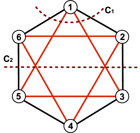
We first study the stability of using (11) as in [19]. By substituting (12) in we find that the edge weights can only take two values:
Then, since any cut that isolates one node from the rest (like in Figure 3) will always have two edges of each type, their sum is zero. Therefore, (11) cannot be used to determine stability.
If we now use condition (10) instead, we are allowed to explore a wider variety of cuts that can potentially have smaller costs. In fact, if instead of we sum over , we obtain,
which implies that is unstable.
Figure 4 verifies the equilibrium instability. By starting with an initial condition close to the equilibrium , we can see how the system slowly starts to move away from towards a stable equilibrium set.
Furthermore, we can study the whole family of non-isolated equilibria given by
| (13) |
where , which due to Remark 3, we can reduce (13) to
| (14) |
with and .
III.2.2 Almost Global Stability
Condition (10) also provides insight on which class of coupling functions can potentially give us almost global convergence to the in-phase equilibrium set . If it is possible to find some with , such that for any non-in-phase equilibrium , there is a cut with , then the in-phase equilibrium set will be almost globally stable [13]. The main difficulty is that for general and arbitrary network , it is not easy to locate every phase-locked equilibria and thus, it is not simple to know in what region of the domain of the slope should be negative.
We now concentrate on the one-parameter family of functions , with , such that whenever is symmetric, odd, continuously differentiable and
- •
, and
- •
.
See Figure 2 for an illustration with . Also note that this definition implies that if , the coupling is attractive and . This last property will be used later. We also assume the graph to be connected.
In order to obtain almost global stability we need to be small. However, since the equilibria position is not known a priori, it is not clear how small should be or if there is any such that all nontrivial equilibria are unstable. We therefore first need to estimate the region of the state space that contains every non-trivial phase-locked solution.
Let be a compact connected subset of and let be its length, e.g., if then . For any and , define as the length of the smallest interval such that , i.e.
Using this metric, together with the aid of Proposition 2.6 of [16] we can identify two very insightful properties of the family whenever the graph is connected.
Claim 1.
If is an equilibrium point of (8) with , then either is an in-phase equilibrium, i.e. for , or has a cut with .
Proof.
Since , all the phases are contained in a half circle and for the oscillator with smallest phase , all the phase differences . However, since implies with equality only for , can only hold if . Now let and . If , then is an in-phase equilibrium. Otherwise, , . ∎
We are now ready to establish a bound on the value of that guarantees the instability of the non-in-phase equilibria.
Claim 2.
Consider and arbitrary connected graph . Then for any and non-in-phase equilibrium , there is a cut with
Proof.
Suppose there is a non-in-phase equilibrium for which no such cut exists. Let and be a partition of for some arbitrary node .
Since such does not exists, there exists some edge , with , such that . Move from one side to the other of the partition by defining and . Now since , then
In other words, both phases should be within a distance smaller than .
Now repeat the argument times. At the iteration, given , , again we can find some , such that and . Also, since at each step ,
Thus by solving the recursion we get:
After iterations we have and . Therefore, since , we obtain
Then, by Claim 1 is either an in-phase equilibrium or there is a cut with . Either case gives a contradiction to assuming that is a non-in-phase equilibrium and does not exists. Therefore, for any non-in-phase and , we can always find a cut with , . ∎
Claim 2 allows us to use our cut condition (10) on every non-in-phase equilibrium. Thus, since (8) is a potential dynamics (c.f. Section III.1.2), from every initial condition the system converges to the set of equilibria . But when the only stable equilibrium set inside is the in-phase set . Thus, set is globally asymptotically stable. We summarized this result in the following Proposition.
Proposition 1 (Almost global stability).
Consider and an arbitrary connected graph . Then, if , the in-phase equilibrium set is almost globally asymptotically stable.
This result provides a sufficient condition for almost global asymptotic stability to the in-phase equilibrium set . Although found independently, the same condition was proposed for a specific piecewise linear in [41]. Here we extend [41] in many aspects. For example, instead of assuming equal coupling for every edge, our condition describes a large family of coupling functions where each can be taken independently from . Also, in [41] the construction of assumes a discontinuity on the derivative at . This can pose a problem if the equilibrium happens to have phase differences . Here we do not have such problem as is continuously differentiable.
The condition implies that, when is large, should be decreasing in most of it domain. Using (4) this implies that should be increasing within the region , which is similar to the condition on [20] and equivalent when . Thus, Proposition 1 confirms the conjecture of [20] by extending their result to arbitrary topologies and a more realistic continuous for the system (1) in the weak coupling limit.
III.3 Complete Graph Topology with a Class of Coupling Functions
In this subsection we investigate how conservative the value of found in Section III.2.2 is for the complete graph topology. We are motivated by the results of [19] where it is shown that () with complete graph topology ensures almost global synchronization.
Since for general it is not easy to characterize all the possible equilibria of the system, we study the stability of the equilibria that appear due to the equivalence of (8) with respect to the action group , where is the group of permutations of the coordinates and represents the group action of phase shift of all the coordinates, i.e. the action of is . We refer the readers to [12] and [16] for a detailed study of the effect of this property.
These equilibria are characterized by the isotropy subgroups of that keep them fixed, i.e., . In [12] it was shown that this isotropy subgroup takes the form of
where and are positive integers such that , is the permutation subgroup of of -many coordinates and is the cyclic group with action . The semiproduct represents the fact that does not commute with the other subgroups.
In other words, each equilibria with isotropy is conformed by shifted constellations () of evenly distributed blocks, with oscillators per block. We use to denote the phase shift between constellation and . See Figure 6 for examples these types of equilibria.

Here we will show that under mild assumptions on and for most of the equilibria found with these characteristics are unstable. We first study all the equilibria with even. In this case there is a special property that can be exploited.
That is, when such that is even around , we have
| (15) | ||||
where the third step comes from being even around and -periodic, and the fourth from being odd.
Having is the key to prove the instability of every equilibria with even . It essentially states that the aggregate effect of one constellation on any oscillator is zero when is even, and therefore any perturbation that maintains has null effect on . This is shown in the next proposition.
Proposition 2 (Instability for even ).
Given an equilibrium with isotropy and even around . Then, if is even, is unstable.
Proof.
We will show the instability of by finding a cut of the network satisfying (10). Let be the set of nodes within one of the blocks of the constellation and consider the partition induced by , i.e. . Due to the structure of , (10) becomes
where is the derivative of and is the phase shift between the and . Finally, since by assumptions then it follows that and
Therefore, by (10), is unstable. ∎
The natural question that arises is whether similar results can be obtained for odd. The main difficulty in this case is that does not hold since we no longer evaluate at points with phase difference equal to such that they cancel each other. Therefore, an extra monotonicity condition needs to be added in order to partially answer this question. These conditions and their effects are summarized in the following claims.
Claim 3 (Monotonicity).
Given such that is strictly concave for , then
| (16) | |||
| (17) |
Proof.
The proof is a direct consequence of the strict concavity of . Since is strictly concave then basic convex analysis shows that is strictly decreasing within . Therefore, the inequality (16) follows directly from the fact that , and . To show (17) it is enough to notice that since is odd ( ), is strictly convex in . The rest of the proof is analogous to (16). ∎
Claim 4 ( Concavity).
Given such that is strictly concave for . Then for all , .
Proof.
Since is concave for then it follows
where . Thus, for , and
as desired. ∎
Now we show the instability of any equilibria with isotropy for odd and greater or equal to .
Proposition 3 (Instability for and odd).
Suppose with concave in and concave in , then for all with the equilibria s with isotropy are unstable.
The proof of Proposition 3 also uses our cut condition to show instability, but with a different cut induced by the partition of where is set to the a maximal subset of such that , see Figure 8 for an illustration of . Notice that any of these partitions will include all the oscillators of two consecutive blocks of every constellation. The details of the proofs are rather technical and are relegated to Appendix A.
IV Effect of Delay
Once delay is introduced to the system of coupled oscillators, the problem becomes fundamentally harder. For example, for pulse-coupled oscillators, the reception of a pulse no longer gives accurate information about the relative phase difference between the two interacting oscillators. Before, at the exact moment when received a pulse from , was zero and the phase difference was estimated locally by as . However, now when receives the pulse, the difference becomes . Therefore, the delay propagation acts as an error introduced to the phase difference measurement and unless some information is known about this error, it is not possible to predict the behavior. Moreover, as we will see later, slight changes in the distribution can produce nonintuitive behaviors.
Even though it may not be satisfactory for some applications, many existing works choose to ignore delay. (see for e.g., [20, 18, 19]). That is mainly for analytical tractability. On the other hand, when delay is included [26] the studies concentrate on finding bounds on delay that maintain stability.
In this section we study how delay can change the stability in a network of weakly coupled oscillators. A new framework to study these systems with delay will be set up by constructing an equivalent non-delayed system that has the same behavior as the original one in the continuum limit. We then further use this result to show that large heterogeneous delay can help reach synchronization, which is a bit counterintuitive and significantly generalizes previous related studies [28, 42, 43]. We will assume complete graph to simplify notation and exposition although the results can be extended for a boarder class of densely connected networks.
The contribution of this section is two fold. First, it improves the understanding of the effect of delays in networks of coupled oscillators. And second, it opens new possibilities of using delay based mechanisms to increase the region of attraction of the in-phase equilibrium set. We shall build on existing arguments such as mean field approximation [33] and Lyapunov stability theory [19, 17] while looking at the problem from a different perspective.
IV.1 Mean Field Approximation
Consider the case where the coupling between oscillators is all to all and identical (, and ). And assume the phase lags are randomly and independently chosen from the same distribution with probability density . By letting and while keeping a constant, (3) becomes
| (18) |
where is a time-variant normalized phase distribution that keeps track of the fraction of oscillators with phase at time , and is the velocity field that expresses the net force that the whole population applies to a given oscillator with phase at time . Since the number of oscillators is preserved at any time, the evolution of is governed by the continuity equation
| (19) |
with the boundary conditions . Equations (18)-(19) are not analytically solvable in general. Here we propose a new perspective that is inspired by the following observation.
Consider the non-delayed system of the form
| (20) |
where
| (21) |
is the convolution between and .
By the same reasoning of (18) it is easy to see that the limiting velocity field of (20) is
where in the first and the third steps we used (21) and (18) respectively. Therefore, (3) and (20) have the same continuum limit.
Remark 4.
Figure 9 shows how, the underlying delay (in this case the delay distribution) determines what type of coupling (attractive or repulsive) produces synchronization. The original function produces repulsive coupling, whereas the corresponding is attractive. In fact, as we will soon see, the distribution of delay not only can qualitatively affect the type of coupling but also can change the stability of certain phase-locked limit cycles.
We now study two example to illustrate how this new approximation can provide significant information about performance and stability of the original system. We also provide numerical simulations to verify our predictions.
IV.2 Kuramoto Oscillators
We start by studying an example in the literature [44] to demonstrate how we can use the previous equivalent non-delayed formulation to provide a better understanding of systems of coupled oscillators with delay. When , can be easily calculated:
where is the imaginary part of a complex number, i.e. . The values of and are calculated using the identity
This complex number, usually called “order parameter”, provides a measure of how the phase-lags are distributed within the unit circle. It can also be interpreted as the center of mass of the lags ’s when they are thought of as points () within the unit circle . Thus, when , the ’s are mostly concentrated around . When , the delay is distributed such that .
In this example, (20) becomes
| (22) |
Here we see how the distribution of has a direct effect on the dynamics. For example, when the delays are heterogeneous enough such that , the coupling term disappears and therefore makes synchronization impossible. A complete study of the system under the context of superconducting Josephson arrays was performed [44] for the complete graph topology. There the authors characterized the condition for in-phase synchronization in terms of and . More precisely, when is on the right half of the plane (), the system almost always synchronizes. However, when is on the left half of the plane (), the system moves towards an incoherent state where all of the oscillators’ phases spread around the unit circle such that its order parameter, i.e. becomes zero.


We now provide simulation results to illustrate how (22) becomes a good approximation of the original system when is large enough. We simulate the original repulsive () sine-coupled system with heterogeneous delays and its corresponding approximation (22). Two different delay distributions, depicted in Figure 10, were selected such that their corresponding order parameter lie in different half-planes.
The same simulation is repeated for . Figure 11 shows that when is small, the phases’ order parameter of the original system (in red/blue) draw a trajectory which is completely different with respect to its approximation (in green). However, as grows, in both cases the trajectories become closer and closer. Since , the trajectory of the system with wider distribution () drives the order parameter towards the boundary of the circle, i.e., heterogeneous delay leads to homogeneous phase.
IV.3 Effect of Heterogeneity
We now explain a more subtle effect that heterogeneity can produce. Consider the system in (20) where odd and continuously differentiable. Then, from Section III, all of the oscillators eventually end up running at the same speed with fixed phase difference such that the sum cancels . Moreover, we can apply (10) to assess the stability of these orbits. Therefore, if we can find a cut of the network such that the phase-locked solution will be unstable.
Although this condition is for non-delayed phase-coupled oscillators, the result of this section allows us to translate it for systems with delay. Since is the convolution of the coupling function and the delay distribution function , we can obtain , even when . This usually occurs when the convolution widens the region with a negative slope of . See Figure 9 for an illustration of this phenomenon.


Figures 12 and 13 show two simulation setups of 45 oscillators pulse-coupled all to all. The initial state is close to a phase locked configuration formed of three equidistant clusters of 15 oscillators each. The shape of the coupling function and the phase lags distributions are shown in part a. We used (4) to implement the corresponding pulse-coupled system (). While is maintained unchanged between both simulations, the distribution does change. Thus, the corresponding changes as it can be seen in part b; the blue, red, and green dots correspond to the speed change induced in an oscillator within the blue cluster by oscillators of each cluster. Since all clusters have the same number of oscillators, the net effect is zero. In part c the time evolution of oscillators’ phases relative to the phase of a blue cluster oscillator are shown. Although the initial conditions are exactly the same, the wider delay distribution on Figure 13 produces negative slope on the red and green points of part b, which destabilizes the clusters and drives oscillators toward in-phase synchrony.
Finally, we simulate the same scenario as in Figures 12 and 13 but now changing and the standard deviation, i.e. the delay distribution width. Figure 14 shows the computation of the synchronization probability vs. standard deviation. The dashed line denotes the minimum value that destabilizes the equivalent system. As grows, the distribution shape becomes closer to a step, which is the expected shape in the limit. It is quite surprising that as soon as the equilibrium is within the region of with negative slope, the equilibrium becomes unstable as the theory predicts.

V Conclusion
This paper analyzes the dynamics of identical weakly coupled oscillators while relaxing several classical assumptions on coupling, delay and topology. Our results provide global synchronization guarantee for a wide range of scenarios. There are many directions that can be taken to further this study. For example, for different topologies, to guarantee global in-phase synchronization, how does the requirement on coupling functions change? Another specific question is to complete the proof in Section III.3 for the cases when . Finally, it will be of great interest if we can apply results and techniques in this paper to a wide range of applications such as transient stability analysis of power networks and clock synchronization of computer networks.
Acknowledgments: The authors thank Steven H. Strogatz of Cornell for useful discussions.
Appendix A Proof of Proposition 3
As in Proposition 2 we will use our cut condition to show the instability of . Thus, we define a partition of by taking to be a maximal subset of such that , see Figure 8 for an illustration of . Notice that any of these partitions will include all the oscillators of two consecutive blocks of every constellation.
Instead of evaluating the total sum of the weights in the cut we will show that the sum of edge weights of the links connecting the nodes of one constellation in with the nodes of a possibly different constellation in is negative. In other words, we will focus on showing
| (23) |
where .
Given any subset of integers , we define
Then, we can rewrite (23) as
| (24) |
where is the phase shift between the two constellations. Then, if we can show that for all (24) is less than zero then for any values of and we will have (23) satisfied.
Since is odd and even around , is even and odd around and can be rewritten as
where is the indicator function of the event , the sum is over all the integers with and
The last term only appears when is odd and in fact it is easy to show that it is always negative as the following calculation shows:
where in step one we used the fact of being even, in step two we used and in step three we use being odd around . The last step comes from substituting , and apply Claim 3, since for we have .
Then it remains the show that the terms of the form are negative for all s.t. . This is indeed true when is positive since for all we get
and thus we can apply again Claim 3.
When is negative there is one exception in which Claim 3 cannot be used since
only holds for . Thus the term corresponding to cannot be directly eliminated.
Then, by keeping only the terms of the sum with , is strictly upper bounded for all by
| (25) |
Finally, since for is strictly increasing and achieves its minimum for , then
where the last inequality follow from Claim 4.
Therefore, for all odd greater or equal to we obtain
and since this result is independent on the indices , , then
and thus is unstable.
References
- [1] A. T. Winfree, “Biological rhythms and the behavior of populations of coupled oscillators,” Journal of Theoretical Biology, vol. 16, no. 1, pp. 15 – 42, 1967.
- [2] C. S. Peskin, Mathematical aspects of heart physiology. New York, NY, USA: Courant Institute of Mathematical Sciences, New York University, 1975.
- [3] P. Achermann and H. Kunz, “Modeling circadian rhythm generation in the suprachiasmatic nucleus with locally coupled self-sustained oscillators: Phase shifts and phase response curves,” Journal of Biological Rhythms, vol. 14, no. 6, pp. 460 – 468, 1999.
- [4] J. Garcia-Ojalvo, M. B. Elowitz, S. H. Strogatz, and C. S. Peskin, “Modeling a synthetic multicellular clock: Repressilators coupled by quorum sensing,” Proceedings of the National Academy of Sciences of the United States of America, vol. 101, no. 30, pp. 10955–10960, 2004.
- [5] S. Yamaguchi, H. Isejima, T. Matsuo, R. Okura, K. Yagita, M. Kobayashi, and H. Okamura, “Synchronization of cellular clocks in the suprachiasmatic nucleus,” Science, vol. 32, pp. 1408–1412, Nov. 2003.
- [6] I. Z. Kiss, Y. Zhai, and J. L. Hudson, “Emerging coherence in a population of chemical oscillators,” Science, vol. 296, pp. 1676–1678, Nov. 2002.
- [7] R. York and R. Compton, “Quasi-optical power combining using mutually synchronized oscillator arrays,” IEEE Transactions on Microwave Theory and Techniques, vol. 39, pp. 1000–1009, Jun. 1991.
- [8] Y.-W. Hong and A. Scaglione, “A scalable synchronization protocol for large scale sensor networks and its applications,” IEEE Journal on Selected Areas in Communications, vol. 23, pp. 1085–1099, May. 2005.
- [9] G. Werner-Allen, G. Tewari, A. Patel, M. Welsh, and R. Nagpal, “Firefly-inspired sensor network synchronicity with realistic radio effects,” in SenSys: Proceedings of the 3rd International Conference on Embedded Networked Sensor Systems, (New York, NY, USA), pp. 142–153, ACM, 2005.
- [10] S. A. Marvel and S. H. Strogatz, “Invariant submanifold for series arrays of josephson junctions,” Chaos, vol. 19, p. 013132, Mar. 2009.
- [11] P. C. Bressloff and S. Coombes, “Travelling waves in chains of pulse-coupled integrate-and-fire oscillators with distributed delays,” Phys. D, vol. 130, no. 3-4, pp. 232–254, 1999.
- [12] P. Ashwin and J. W. Swift, “The dynamics of n weakly coupled identical oscillators,” J. Nonlinear Sci, vol. 2, no. 1, pp. 69–108, 1992.
- [13] G. B. Ermentrout, “Stable periodic solutions to discrete and continuum arrays of weakly coupled nonlinear oscillators,” SIAM J. Appl. Math., vol. 52, no. 6, pp. 1665–1687, 1992.
- [14] Y. Kuramoto, “International symposium on mathematical problems in theoretical physics,” in Lecture notes in Physics, vol. 39, p. 420, Springer, 1975.
- [15] O. V. Popovych, Y. L. Maistrenko, and P. A. Tass, “Phase chaos in coupled oscillators,” Phys. Rev. E, vol. 71, p. 065201, Jun. 2005.
- [16] E. Brown, P. Holmes, and J. Moehlis, “Globally coupled oscillator networks,” in Perspectives and Problems in Nonlinear Science: A Celebratory Volume in Honor of Larry Sirovich, pp. 183–215, Springer, 2003.
- [17] A. Jadbabaie, N. Motee, and M. Barahona, “On the stability of the kuramoto model of coupled nonlinear oscillators,” in Proceedings of the American Control Conference., vol. 5, pp. 4296–4301, June 30, 2004.
- [18] D. Lucarelli and I.-J. Wang, “Decentralized synchronization protocols with nearest neighbor communication,” in Proceedings of the 2nd International Conference on Embedded Networked Sensor Systems, 2004.
- [19] P. Monzón and F. Paganini, “Global considerations on the kuramoto model of sinusoidally coupled oscillators,” in Proceedings of the 44th IEEE Conference on Decision and Control, and European Control Conference, (Sevilla, Spain), pp. 3923–3928, Dec. 2005.
- [20] R. E. Mirollo and S. H. Strogatz, “Synchronization of pulse-coupled biological oscillators.,” SIAM J. Appl. Math, vol. 50, pp. 1645–1662, 1990.
- [21] L. Moreau, “Stability of continuous-time distributed consensus algorithms,” in Decision and Control, 2004. CDC. 43rd IEEE Conference on, vol. 4, pp. 3998 – 4003 Vol.4, dec. 2004.
- [22] W. Ren and R. Beard, “Consensus of information under dynamically changing interaction topologies,” in American Control Conference, 2004. Proceedings of the 2004, vol. 6, pp. 4939 –4944 vol.6, 30 2004-july 2 2004.
- [23] G.-B. Stan and R. Sepulchre, “Dissipativity characterization of a class of oscillators and networks of oscillators,” in Decision and Control, 2003. Proceedings. 42nd IEEE Conference on, vol. 4, pp. 4169 – 4173 vol.4, dec. 2003.
- [24] L. Scardovi, A. Sarlette, and R. Sepulchre, “Synchronization and balancing on the n-torus,” Systems & Control Letters, vol. 56, no. 5, pp. 335 – 341, 2007.
- [25] R. Sepulchre, D. A. Paley, and N. E. Leonard, “Stabilization of planar collective motion with limited communication,” Automatic Control, IEEE Transactions on, vol. 53, no. 3, pp. 706–719, 2008.
- [26] A. Papachristodoulou and A. Jadbabaie, “Synchonization in oscillator networks with heterogeneous delays, switching topologies and nonlinear dynamics,” in Proceedings of the 45th IEEE Conference on Decision and Control, pp. 4307–4312, Dec. 2006.
- [27] E. M. Izhikevich, “Phase models with explicit time delays,” Phys. Rev. E, vol. 58, pp. 905–908, Jul. 1998.
- [28] E. M. Izhikevich, “Weakly pulse-coupled oscillators, fm interactions, synchronization, and oscillatory associative memory,” IEEE Transactions on Neural Networks, vol. 10, pp. 508–526, May. 1999.
- [29] E. Mallada and A. Tang, “Synchronization of phase-coupled oscillators with arbitrary topology,” in Proceedings of American Control Conference, 2010.
- [30] E. Mallada and A. Tang, “Weakly pulse-coupled oscillators: Heterogeneous delays lead to homogeneous phase,” in IEEE Conference on Decision and Control, 2010.
- [31] U. Ernst, K. Pawelzik, and T. Geisel, “Synchronization induced by temporal delays in pulse-coupled oscillators,” Phys. Rev. Lett., vol. 74, pp. 1570–1573, Feb. 1995.
- [32] U. Ernst, K. Pawelzik, and T. Geisel, “Delay-induced multistable synchronization of biological oscillators,” Phys. Rev. E, vol. 57, pp. 2150–2162, Feb. 1998.
- [33] Y. Kuramoto, Chemical Oscillations, Waves, and Turbulence. Berin Heidelberg New York Tokyo: Springer-Verlag, 1984.
- [34] R. Sepulchre, D. A. Paley, and N. E. Leonard, “Stabilization of planar collective motion: All-to-all communication,” Automatic Control, IEEE Transactions on, vol. 52, no. 5, pp. 811–824, 2007.
- [35] H. Daido, “Quasientrainment and slow relaxation in a population of oscillators with random and frustrated interactions,” Phys. Rev. Lett., vol. 68, pp. 1073–1076, Feb 1992.
- [36] A. Rantzer, “A dual to lyapunov’s stability theorem,” Systems and Control Letters, vol. 42, pp. 161–168, 2001.
- [37] B. Bollobas, Modern Graph Theory. New York: Springer, 1998.
- [38] C. Godsil and G. Royle, Algebraic Graph Theory. New York: Springer, 2001.
- [39] H. K. Khalil, Nonlinear systems; 3rd ed. Prentice-Hall, 1996.
- [40] F. C. Hoppensteadt and E. M. Izhikevich, “Weakly connected neural networks,” 1997.
- [41] A. Sarlette, Geometry and symmetries in coordination control. PhD thesis, University of Liège, Belgium, January 2009.
- [42] C. van Vreeswijk, L. Abbott, and G. B. Ermentrout, “When inhibition not excitation synchronizes neural firing,” Journal of Computational Neuroscience, vol. 1, no. 4, pp. 313–321, 1994.
- [43] W. Gerstner, “Rapid phase locking in systems of pulse-coupled oscillators with delays,” Phys. Rev. Lett., vol. 76, pp. 1755–1758, Mar 1996.
- [44] S. Watanabe and S. H. Strogatz, “Constants of motion for superconducting josephson arrays,” Phys. D, vol. 74, no. 3-4, pp. 197–253, 1994.