跳到论文正文
W Papers独立论文阅读器 arXiv:1303.7247 论文正文 计算阅读时间 · 0%
引用这篇论文根据当前论文元数据生成,正式投稿前建议核对。


License: arXiv.org perpetual non-exclusive license
arXiv:1303.7247v5 [math.OC] 17 Mar 2015

THE LOG-EXPONENTIAL SMOOTHING TECHNIQUE AND NESTEROV’S ACCELERATED GRADIENT METHOD FOR GENERALIZED SYLVESTER PROBLEMS
N.T. An11 1 Thua Thien Hue College of Education, 123 Nguyen Hue, Hue City, Vietnam (email: thaian2784@gmail.com)., D. Giles22 2 Fariborz Maseeh Department of Mathematics and Statistics, Portland State University, PO Box 751, Portland, OR 97207, United States (email: dangiles@pdx.edu). The research of Daniel Giles was partially supported by the USA National Science Foundation under grant DMS-1411817., N.M. Nam33 3 Fariborz Maseeh Department of Mathematics and Statistics, Portland State University, PO Box 751, Portland, OR 97207, United States (email: mau.nam.nguyen@pdx.edu). The research of Nguyen Mau Nam was partially supported by the USA National Science Foundation under grant DMS-1411817 and the Simons Foundation under grant #208785., R. B. Rector44 4 Fariborz Maseeh Department of Mathematics and Statistics, Portland State University, PO Box 751, Portland, OR 97207, United States (email: r.b.rector@pdx.edu).

Abstract: The Sylvester smallest enclosing circle problem involves finding the smallest circle that encloses a finite number of points in the plane. We consider generalized versions of the Sylvester problem in which the points are replaced by sets. Based on the log-exponential smoothing technique and Nesterov’s accelerated gradient method, we present an effective numerical algorithm for solving these problems.

Key words. log-exponential smoothing; minimization majorization algorithm; Nesterov’s accelerated gradient method; generalized Sylvester problem.

AMS subject classifications. 49J52, 49J53, 90C31.

1 Introduction

The smallest enclosing circle problem can be stated as follows: Given a finite set of points in the plane, find the circle of smallest radius that encloses all of the points. This problem was introduce in the 19th century by the English mathematician James Joseph Sylvester (1814–1897) [24]. It is both a facility location problem and a major problem in computational geometry. Over a century later, the smallest enclosing circle problem remains very active due to its important applications to clustering, nearest neighbor search, data classification, facility location, collision detection, computer graphics, and military operations. The problem has been widely treated in the literature from both theoretical and numerical standpoints; see [1, 4, 6, 7, 9, 21, 23, 25, 27, 28, 31] and the references therein.

The authors’ recent research focuses on generalized Sylvester problems in which the given points are replaced by sets. Besides the intrinsic mathematical motivation, this question appears in more complicated models of facility location in which the sizes of the locations are not negligible, as in bilevel transportation problems. The main goal of this paper is to develop an effective numerical algorithm for solving the smallest intersecting ball problem. This problems asks for the smallest ball that intersects a finite number of convex target sets in ℝn\mathbb{R}^{n}. Note that when the target sets given in the problem are singletons, the smallest intersecting ball problem reduces to the classical Sylvester problem.

The smallest intersecting ball problem can be solved by minimizing a nonsmooth optimization problem in which the objective function is the maximum of the distances to the target sets. The nondifferentiability of this objective function makes it difficult to develop effective numerical algorithms for solving the problem. A natural approach is to approximate the nonsmooth objective function by a smooth function that is favorable for applying available smooth optimization schemes. Based on the log-exponential smoothing technique and Nesterov’s accelerated gradient method, we present an effective numerical algorithm for solving this problem.

Our paper is organized as follows. Section 2 contains tools of convex optimization used throughout the paper. In Section 3, we focus the analysis of the log-exponential smoothing technique applied to the smallest intersecting ball problem. Section 4 is devoted to developing an effective algorithm based on the minimization majorization algorithm and Nesterov’s accelerated gradient method to solve the problem. We also analyze the convergence of the algorithm. Finally, we present some numerical examples in Section 5.

2 Problem Formulation and Tools of Convex Optimization

In this section, we introduce the mathematical models of the generalized Sylvester problems under consideration. We also present some important tools of convex optimization used throughout the paper.

Consider the linear space ℝn\mathbb{R}^{n} equipped with the Euclidean norm ∥⋅∥\|\cdot\|. The distance function to a nonempty subset QQ of ℝn\mathbb{R}^{n} is defined by

d⁡(x,Q):=inf{‖x−q‖|q∈Q},x∈ℝn.d(x;Q):=\inf\{\|x-q\|\;|\;q\in Q\},\;x\in\mathbb{R}^{n}. (2.1)

Given x∈ℝnx\in\mathbb{R}^{n}, the Euclidean projection from xx to is the set

Π⁡(x,Q):={q∈Q|d⁡(x,Q)=‖x−q‖}.\Pi(x;Q):=\{q\in Q\;|\;d(x;Q)=\|x-q\|\}.

If QQ is a nonempty closed convex set in ℝn\mathbb{R}^{n}, then Π⁡(x,Q)\Pi(x;Q) is a singleton for every x∈ℝnx\in\mathbb{R}^{n}. Furthermore, the projection operator is non-expansive in the sense that

‖Π⁡(x,Q)−Π⁡(y,Q)‖≤‖x−y‖​for all ​x,y∈ℝn.\|\Pi(x;Q)-\Pi(y;Q)\|\leq\|x-y\|\;\mbox{\rm for all }x,y\in\mathbb{R}^{n}.

Let Ω\Omega and Ωi\Omega_{i} for i=1,…,mi=1,\ldots,m be nonempty closed convex subsets of ℝn\mathbb{R}^{n}. The mathematical modeling of the smallest intersecting ball problem with target sets Ωi\Omega_{i} for i=1,…,mi=1,\ldots,m and constraint set Ω\Omega is

minimize 𝒟(x):=max{d(x;Ωi)|i=1,…,m} subject to x∈Ω.\mbox{minimize }\mathcal{D}(x):=\max\big\{d(x;\Omega_{i})\;\big|\;i=1,\ldots,m\big\}\mbox{ subject to }x\in\Omega. (2.2)

The solution to this problem gives the center of the smallest Euclidean ball (with center in Ω\Omega) that intersects all target sets Ωi\Omega_{i} for i=1,…,mi=1,\ldots,m.

In order to study new problems in which the intersecting Euclidean ball is replaced by balls generated by different norms, we consider a more general setting. Let FF be a closed bounded convex set that contains the origin as an interior point. We hold this as our standing assumptions for the set FF for the remainder of the paper. The support function associated with FF is defined by

σF​(x):=sup{⟨x,f⟩|f∈F}.\sigma_{F}(x):=\sup\{\langle x,f\rangle\;|\;f\in F\}.

Note that if F={x∈ℝn|‖x‖X≤1}F=\{x\in\mathbb{R}^{n}\;|\;\|x\|_{X}\leq 1\}, where ∥⋅∥X\|\cdot\|_{X} is a norm in ℝn\mathbb{R}^{n}, then σF\sigma_{F} is the dual norm of the norm ∥⋅∥X\|\cdot\|_{X}.

Let QQ be a nonempty subset of ℝn\mathbb{R}^{n}. The generalized distance from a point x∈ℝnx\in\mathbb{R}^{n} to QQ generated by FF is given by

dF​(x,Q):=inf{σF​(x−q)|q∈Q}.d_{F}(x;Q):=\inf\{\sigma_{F}(x-q)\;|\;q\in Q\}. (2.3)

The generalized distance function (2.3) reduces to the distance function (2.1) when FF is the closed unit ball of ℝn\mathbb{R}^{n} with respect to the Euclidean norm. The readers are referred to [14] for important properties of the generalized distance function (2.3).

Using (2.3), a more general model of problem (2.2) is given by

minimize 𝒟F(x):=max{dF(x;Ωi)|i=1,…,m} subject to x∈Ω.\mbox{minimize }\mathcal{D}_{F}(x):=\max\big\{d_{F}(x;\Omega_{i})\;\big|\;i=1,\ldots,m\big\}\mbox{ subject to }x\in\Omega. (2.4)

The function 𝒟F\mathcal{D}_{F} as well as its specification 𝒟\mathcal{D} are nonsmooth in general. Thus, problem (2.4) and, in particular, problem (2.2) must be studied from both theoretical and numerical view points using the tools of generalized differentiation from convex analysis.

Given a function φ:ℝn→ℝ\varphi\colon\mathbb{R}^{n}\to\mathbb{R}, we say that φ\varphi is convex if it satisfies

φ⁡(λ​x+(1−λ)​y)≤λ​φ​(x)+(1−λ)​φ​(y),\varphi(\lambda x+(1-\lambda)y)\leq\lambda\varphi(x)+(1-\lambda)\varphi(y),

for all x,y∈ℝnx,y\in\mathbb{R}^{n} and λ∈(0,1)\lambda\in(0,1). The function φ\varphi is said to be strictly convex if the above inequality becomes strict whenever x≠yx\neq y.

The class of convex functions plays an important role in many applications of mathematics, especially applications to optimization. It is well-known that for a convex function f:ℝn→ℝf:\mathbb{R}^{n}\to\mathbb{R}, the function has an absolute minimum on a convex set Ω\Omega at x¯\bar{x} if and only if it has a local minimum on Ω\Omega at x¯\bar{x}. Moreover, if f:ℝn→ℝf:\mathbb{R}^{n}\to\mathbb{R} is a differentiable convex function, then x¯∈Ω\bar{x}\in\Omega is a minimizer for ff if and only if

⟨∇f​(x¯),x−x¯⟩≥0​for all ​x∈Ω.\langle\nabla f(\bar{x}),x-\bar{x}\rangle\geq 0\;\mbox{\rm for all }x\in\Omega. (2.5)

The readers are referred to [2, 3, 10, 15] for more complete theory of convex analysis and applications to optimization from both theoretical and numerical aspects.

3 Smoothing Techniques for Generalized Sylvester Problems

In this section, we employ the approach developed in [31] to approximate the nonsmooth optimization problem (2.4) by a smooth optimization problem which is favorable for applying available smooth numerical algorithms. The difference here is that we use generalized distances to sets instead of distances to points.

Given an element v∈ℝnv\in\mathbb{R}^{n}, the cone generated by vv is given by cone​{v}:={λ​v|λ≥0}.\mbox{\rm cone}\,\{v\}:=\{\lambda v\;|\;\lambda\geq 0\}. Let us review the following definition from [14]. We recall that FF is a closed bounded convex set that contains zero in its interior, as per the standing assumptions in this paper.

Definition 3.1

The set FF is normally smooth if for every x∈bd​Fx\in\mbox{\rm bd}\,F there exists ax∈ℝna_{x}\in\mathbb{R}^{n} such that N⁡(x,F)=cone​{ax}N(x;F)=\mbox{\rm cone}\,\{a_{x}\}.

In the theorem below, we establish the necessary and sufficient condition for the smallest intersecting ball problem (2.4) to have a unique optimal solution.

Theorem 3.2

Suppose that FF is normally smooth, all of the target sets are strictly convex, and at least one of the sets Ω,Ω1,…,Ωm\Omega,\Omega_{1},...,\Omega_{m} is bounded. Then the smallest intersecting ball problem (2.4) has a unique optimal solution if and only if ⋂i=1m(Ω∩Ωi)\bigcap_{i=1}^{m}\left(\Omega\cap\Omega_{i}\right) contains at most one point.

Proof It is clear that every point in the set ⋂i=1m(Ω∩Ωi)\bigcap_{i=1}^{m}\left(\Omega\cap\Omega_{i}\right) is a solution of (2.4). Thus, if (2.4) has a unique optimal solution we must have that ⋂i=1m(Ω∩Ωi)\bigcap_{i=1}^{m}\left(\Omega\cap\Omega_{i}\right) contains at most one point, so the necessary condition has been proven.

For the sufficient condition, assume that ⋂i=1m(Ω∩Ωi)\bigcap_{i=1}^{m}\left(\Omega\cap\Omega_{i}\right) contains at most one point. The existence of an optimal solution is guaranteed by the assumption that at least one of the sets Ω,Ω1,…,Ωm\Omega,\Omega_{1},...,\Omega_{m} is bounded. What remains to be shown is the uniqueness of this solution. We consider two cases.

In the first case, we assume that ⋂i=1m(Ω∩Ωi)\bigcap_{i=1}^{m}\left(\Omega\cap\Omega_{i}\right) contains exactly one point x¯\bar{x}. Observe that 𝒟F​(x¯)=0\mathcal{D}_{F}(\bar{x})=0 and 𝒟F​(x)≥0\mathcal{D}_{F}(x)\geq 0 for all x∈ℝnx\in\mathbb{R}^{n}, so x¯\bar{x} is a solution of (2.4). If x^∈Ω\hat{x}\in\Omega is another solution then we must have 𝒟F​(x^)=𝒟F​(x¯)=0\mathcal{D}_{F}(\hat{x})=\mathcal{D}_{F}(\bar{x})=0. Therefore, dF​(x^,Ωi)=0d_{F}(\hat{x};\Omega_{i})=0 for all i∈{1,…,m}i\in\{1,\ldots,m\} and hence x^∈⋂i=1m(Ω∩Ωi)={x¯}\hat{x}\in\bigcap_{i=1}^{m}\left(\Omega\cap\Omega_{i}\right)=\{\bar{x}\}. We conclude that x^=x¯\hat{x}=\bar{x} and the problem has unique solution in this case.

For the second case we assume that ⋂i=1m(Ω∩Ωi)=∅\bigcap_{i=1}^{m}\left(\Omega\cap\Omega_{i}\right)=\emptyset. We will show that the function

S⁡(x)=max⁡{(dF​(x,Ω1))2,…,(dF​(x,Ωm))2},S(x)=\max\{\left(d_{F}(x;\Omega_{1})\right)^{2},\ldots,\left(d_{F}(x;\Omega_{m})\right)^{2}\},

is strictly convex on Ω\Omega. This will prove the uniqueness of the solution.

Take any x,y∈Ωx,y\in\Omega, x≠yx\neq y and t∈(0,1)t\in(0,1). Denote xt:=t​x+(1−t)​yx_{t}:=tx+(1-t)y. Let i∈{1,…,m}i\in\{1,\ldots,m\} such that (dF​(xt,Ωi))2=S⁡(xt)\left(d_{F}(x_{t};\Omega_{i})\right)^{2}=S(x_{t}). Let u,v∈Ωiu,v\in\Omega_{i} such that σF​(x−u)=dF​(x,Ωi)\sigma_{F}(x-u)=d_{F}(x;\Omega_{i}) and σF​(y−v)=dF​(y,Ωi)\sigma_{F}(y-v)=d_{F}(y;\Omega_{i}). Then we have

S⁡(xt)\displaystyle S(x_{t}) =(dF​(xt,Ωi))2\displaystyle=\left(d_{F}(x_{t};\Omega_{i})\right)^{2}
=[dF​(t​x+(1−t)​y,Ωi)]2\displaystyle=\left[d_{F}(tx+(1-t)y;\Omega_{i})\right]^{2}
≤[t​dF​(x,Ωi)+(1−t)​dF​(y,Ωi)]2\displaystyle\leq\left[td_{F}(x;\Omega_{i})+(1-t)d_{F}(y;\Omega_{i})\right]^{2}
=[t​σF​(x−u)+(1−t)​σF​(y−v)]2\displaystyle=\left[t\sigma_{F}(x-u)+(1-t)\sigma_{F}(y-v)\right]^{2}
=t2​(σF​(x−u))2+2​t​(1−t)​σF​(x−u)​σF​(y−v)+(1−t)2​(σF​(y−v))2\displaystyle=t^{2}\left(\sigma_{F}(x-u)\right)^{2}+2t(1-t)\sigma_{F}(x-u)\sigma_{F}(y-v)+(1-t)^{2}\left(\sigma_{F}(y-v)\right)^{2}
≤t2​(σF​(x−u))2+t⁡(1−t)​[(σF​(x−u))2+(σF​(y−v)2)]+(1−t)2​(σF​(y−v))2\displaystyle\leq t^{2}\left(\sigma_{F}(x-u)\right)^{2}+t(1-t)\left[\left(\sigma_{F}(x-u)\right)^{2}+\left(\sigma_{F}(y-v)^{2}\right)\right]+(1-t)^{2}\left(\sigma_{F}(y-v)\right)^{2}
=t​(σF​(x−u))2+(1−t)​(σF​(y−v))2\displaystyle=t\left(\sigma_{F}(x-u)\right)^{2}+(1-t)\left(\sigma_{F}(y-v)\right)^{2}
=t​(dF​(x,Ωi))2+(1−t)​(dF​(y,Ωi))2\displaystyle=t\left(d_{F}(x;\Omega_{i})\right)^{2}+(1-t)\left(d_{F}(y;\Omega_{i})\right)^{2}
≤t​S​(x)+(1−t)​S​(y).\displaystyle\leq tS(x)+(1-t)S(y).

Recall that we need to prove the inequality S⁡(xt)<t​S​(x)+(1−t)​S​(y)S(x_{t})<tS(x)+(1-t)S(y). Suppose by contradiction that S⁡(xt)=t​S​(x)+(1−t)​S​(y)S(x_{t})=tS(x)+(1-t)S(y). Then all of the inequalities in the above estimate are turned to equalities and thus we have

dF​(xt,Ωi)=t​dF​(x,Ωi)+(1−t)​dF​(y,Ωi)d_{F}(x_{t};\Omega_{i})=td_{F}(x;\Omega_{i})+(1-t)d_{F}(y;\Omega_{i})

and

σF​(x−u)=σF​(y−v).\sigma_{F}(x-u)=\sigma_{F}(y-v). (3.6)

Hence,

dF​(xt,Ωi)=σF​(x−u)=σF​(y−v).d_{F}(x_{t};\Omega_{i})=\sigma_{F}(x-u)=\sigma_{F}(y-v). (3.7)

Observe that σF​(w)=0\sigma_{F}(w)=0 if and only if w=0w=0, (3.7) implies x=ux=u if and only if y=vy=v. We claim that x≠ux\neq u and y≠vy\neq v. Indeed, if x=ux=u and y=vy=v, then x,y∈Ωix,y\in\Omega_{i} and hence xt∈Ωix_{t}\in\Omega_{i} by the convexity of Ωi\Omega_{i}. Thus dF​(xt,Ωi)=0d_{F}(x_{t};\Omega_{i})=0. This contradicts the fact that dF​(xt,Ωi)=𝒟F​(xt)>0d_{F}(x_{t};\Omega_{i})=\mathcal{D}_{F}(x_{t})>0 which guaranteed by the assumption ⋂i=1m(Ω∩Ωi)=∅\bigcap_{i=1}^{m}\left(\Omega\cap\Omega_{i}\right)=\emptyset.

Now, we will show that u≠vu\neq v. Denote c:=t​u+(1−t)​v∈Ωic:=tu+(1-t)v\in\Omega_{i}. The properties of the support function and (3.6) give

dF​(xt,Ωi)\displaystyle d_{F}(x_{t};\Omega_{i}) ≤σF​(xt−c)\displaystyle\leq\sigma_{F}\left(x_{t}-c\right)
=σF​(t⁡(x−u)+(1−t)​(y−v))\displaystyle=\sigma_{F}\left(t(x-u)+(1-t)(y-v)\right)
≤σF​(t⁡(x−u))+σF​((1−t)​(y−v))\displaystyle\leq\sigma_{F}\left(t(x-u)\right)+\sigma_{F}\left((1-t)(y-v)\right)
≤t​σF​(x−u)+(1−t)​σF​(y−v)\displaystyle\leq t\sigma_{F}(x-u)+(1-t)\sigma_{F}(y-v)
=σF​(x−u).\displaystyle=\sigma_{F}(x-u).

By (3.7) we have σF​(t⁡(x−u)+(1−t)​(y−v))=σF​(t⁡(x−u))+σF​((1−t)​(y−v)).\sigma_{F}\left(t(x-u)+(1-t)(y-v)\right)=\sigma_{F}\left(t(x-u)\right)+\sigma_{F}\left((1-t)(y-v)\right). Since FF is normally smooth, it follows from [14, Remark 3.4] that there exists λ>0\lambda>0 satisfying

t⁡(x−u)=λ⁡(1−t)​(y−v).t(x-u)=\lambda(1-t)(y-v).

Now, by contradiction, suppose u=vu=v. Then x−u=β⁡(y−u)x-u=\beta(y-u) where β=t−1​λ​(1−t)\beta=t^{-1}\lambda(1-t). Note that β≠1\beta\neq 1 since x≠yx\neq y and σF​(y−u)>0\sigma_{F}(y-u)>0 since y−u≠0y-u\neq 0. Now we have

σF​(x−u)\displaystyle\sigma_{F}(x-u) =sup{⟨x−u,f⟩|f∈F}=sup{⟨β⁡(y−u),f⟩|f∈F}\displaystyle=\sup\{\langle x-u,f\rangle\;|\;f\in F\}=\sup\{\langle\beta(y-u),f\rangle\;|\;f\in F\}
=β​sup{⟨y−u,f⟩|f∈F}=β​σF​(y−u)≠σF​(y−u),\displaystyle=\beta\sup\{\langle y-u,f\rangle\;|\;f\in F\}=\beta\sigma_{F}(y-u)\neq\sigma_{F}(y-u),

which contradicts (3.7). Thus u≠vu\neq v.

Since u,v∈Ωiu,v\in\Omega_{i}, u≠vu\neq v and Ωi\Omega_{i} is strictly convex, c∈int ​Ωic\in\mbox{int }\Omega_{i}. The assumption ⋂i=1m(Ω∩Ωi)=∅\bigcap_{i=1}^{m}\left(\Omega\cap\Omega_{i}\right)=\emptyset gives dF​(xt,Ωi)=𝒟F​(xt)>0d_{F}(x_{t};\Omega_{i})=\mathcal{D}_{F}(x_{t})>0. Therefore, xt∉Ωix_{t}\notin\Omega_{i} and thus xt≠cx_{t}\neq c. Let δ>0\delta>0 such that I​B​(c,δ)⊂ΩiI\!\!B(c;\delta)\subset\Omega_{i}. Then c+γ⁡(xt−c)∈Ωic+\gamma(x_{t}-c)\in\Omega_{i}, with γ=δ2​‖xt−c‖>0\gamma=\frac{\delta}{2\|x_{t}-c\|}>0. We have

dF​(xt,Ωi)\displaystyle d_{F}(x_{t};\Omega_{i}) ≤σF​(xt−c−γ⁡(xt−c))=(1−γ)​σF​(t⁡(x−u)+(1−t)​(y−v))\displaystyle\leq\sigma_{F}\left(x_{t}-c-\gamma(x_{t}-c)\right)=(1-\gamma)\sigma_{F}\left(t(x-u)+(1-t)(y-v)\right)
<σF​(t⁡(x−u)+(1−t)​(y−v))=σF​(x−u).\displaystyle<\sigma_{F}\left(t(x-u)+(1-t)(y-v)\right)=\sigma_{F}(x-u).

This contradicts (3.7) and completes the proof. □\hfill\square

Recall the following definition.

Definition 3.3

A convex set FF is said to be normally round if N⁡(x,F)≠N⁡(y,F)N(x;F)\neq N(y;F) whenever x,y∈bd​Fx,y\in\mbox{\rm bd}\,F, x≠yx\neq y.

Proposition 3.4

Let Θ\Theta be a nonempty closed convex subset of ℝn\mathbb{R}^{n}. Suppose that FF is normally smooth and normally round. Then the function g⁡(x):=[dF​(x,Θ)]2g(x):=[d_{F}(x;\Theta)]^{2}, x∈ℝnx\in\mathbb{R}^{n}, is continuously differentiable.

Proof It suffices to show that ∂g⁡(x¯)\partial g(\bar{x}) is a singleton for every x¯∈ℝn\bar{x}\in\mathbb{R}^{n}. By [15], we have

∂g⁡(x¯)=2​dF​(x¯,Θ)​∂dF​(x¯,Θ).\partial g(\bar{x})=2d_{F}(\bar{x};\Theta)\partial d_{F}(\bar{x};\Theta).

It follows from [14, Proposition 4.3 (iii)] that gg is continuously differentiable on Θc\Theta^{c}, and so

∂g(x¯)=2dF(x¯;Θ)∇dF(x¯;Θ)=2dF(x¯;Θ)∇σF(x¯−w),\partial g(\bar{x})=2d_{F}(\bar{x};\Theta)\nabla d_{F}(\bar{x};\Theta)=2d_{F}(\bar{x};\Theta)\nabla\sigma_{F}(\bar{x}-w),

where w:=ΠF​(x¯,Θ)w:=\Pi_{F}(\bar{x};\Theta) and x¯∉Θ\bar{x}\notin\Theta.

In the case where x¯∈Θ\bar{x}\in\Theta, one has dF​(x¯,Θ)=0d_{F}(\bar{x};\Theta)=0, and hence

∂g⁡(x¯)=2​dF​(x¯,Θ)​∂dF​(x¯,Θ)={0}.\partial g(\bar{x})=2d_{F}(\bar{x};\Theta)\partial d_{F}(\bar{x};\Theta)=\{0\}.

The proof is now complete. □\hfill\square

If all of the target sets have a common point which belongs to the constraint set, then such a point is a solution of problem (2.4), so we always assume that ⋂i=1n(Ωi∩Ω)=∅\bigcap_{i=1}^{n}\left(\Omega_{i}\cap\Omega\right)=\emptyset. We also assume that at least one of the sets Ω,Ω1,…,Ωm\Omega,\Omega_{1},...,\Omega_{m} is bounded which guarantees the existence of an optimal solution; see [16]. These are our standing assumptions for the remainder of this section.

Let us start with some useful well-known results. We include the proofs for the convenience of the reader.

Lemma 3.5

Given positive numbers aia_{i} for i=1,…,mi=1,\ldots,m, m>1m>1, and 0<s<t0<s<t, one has
(i) (a1s+a2s+…+ams)1/s>(a1t+a2t+…+amt)1/t(a_{1}^{s}+a_{2}^{s}+\ldots+a_{m}^{s})^{1/s}>(a_{1}^{t}+a_{2}^{t}+\ldots+a_{m}^{t})^{1/t}.
(ii) (a11/s+a21/s+…+am1/s)s<(a11/t+a21/t+…+am1/t)t(a_{1}^{1/s}+a_{2}^{1/s}+\ldots+a_{m}^{1/s})^{s}<(a_{1}^{1/t}+a_{2}^{1/t}+\ldots+a_{m}^{1/t})^{t}.
(iii) limr→0+(a11/r+a21/r+…+am1/r)r=max⁡{a1,…,am}\lim_{r\to 0^{+}}(a_{1}^{1/r}+a_{2}^{1/r}+\ldots+a_{m}^{1/r})^{r}=\max\{a_{1},\ldots,a_{m}\}.

Proof (i) Since t/s>1t/s>1, it is obvious that

(a1s∑i=1mais)t/s+⋯+(ams∑i=1mais)t/s<a1s∑i=1mais+⋯+ams∑i=1mais=1,\Big(\dfrac{a_{1}^{s}}{\sum_{i=1}^{m}a_{i}^{s}}\Big)^{t/s}+\cdots+\Big(\dfrac{a_{m}^{s}}{\sum_{i=1}^{m}a_{i}^{s}}\Big)^{t/s}<\dfrac{a_{1}^{s}}{\sum_{i=1}^{m}a_{i}^{s}}+\cdots+\dfrac{a_{m}^{s}}{\sum_{i=1}^{m}a_{i}^{s}}=1,

since ais∑i=1mais∈(0,1)\dfrac{a_{i}^{s}}{\sum_{i=1}^{m}a_{i}^{s}}\in(0,1). It follows that

a1t(∑i=1mais)t/s+⋯+amt(∑i=1mais)t/s<1,\dfrac{a_{1}^{t}}{(\sum_{i=1}^{m}a_{i}^{s})^{t/s}}+\cdots+\dfrac{a_{m}^{t}}{(\sum_{i=1}^{m}a_{i}^{s})^{t/s}}<1,

and hence

a1t+⋯+amt<(∑i=1mais)t/s.a_{1}^{t}+\cdots+a_{m}^{t}<(\sum_{i=1}^{m}a_{i}^{s})^{t/s}.

This implies (i) by rasing both sides to the power of 1/t1/t.
(ii) Inequality (ii) follows directly from (i).
(iii) Defining a:=max⁡{a1,…,am}a:=\max\{a_{1},\ldots,a_{m}\} yields

a≤(a11/r+a21/r+…+am1/r)r≤mr​a→a​as ​r→0+,a\leq(a_{1}^{1/r}+a_{2}^{1/r}+\ldots+a_{m}^{1/r})^{r}\leq m^{r}a\to a\;\mbox{\rm as }r\to 0^{+},

which implies (iii) and completes the proof. □\hfill\square

For p>0p>0 and for x∈ℝnx\in\mathbb{R}^{n}, the log-exponential smoothing function of 𝒟F​(x)\mathcal{D}_{F}(x) is defined as

𝒟F​(x,p):=p​ln​∑i=1mexp⁡(GF,i​(x,p)p),\mathcal{D}_{F}(x,p):=p\ln\sum_{i=1}^{m}\exp\left(\frac{G_{F,i}(x,p)}{p}\right), (3.8)

where

GF,i​(x,p):=dF​(x,Ωi)2+p2.G_{F,i}(x,p):=\sqrt{d_{F}(x;\Omega_{i})^{2}+p^{2}}.
Theorem 3.6

The function 𝒟F​(x,p)\mathcal{D}_{F}(x,p) defined in (3.8) has the following properties:
(i) If x∈ℝnx\in\mathbb{R}^{n} and 0<p1<p20<p_{1}<p_{2}, then

𝒟F​(x,p1)<𝒟F​(x,p2).\mathcal{D}_{F}(x,p_{1})<\mathcal{D}_{F}(x,p_{2}).

(ii) For any x∈ℝnx\in\mathbb{R}^{n} and p>0p>0,

0≤𝒟F​(x,p)−𝒟F​(x)≤p⁡(1+ln⁡m).0\leq\mathcal{D}_{F}(x,p)-\mathcal{D}_{F}(x)\leq p(1+\ln m).

(iii) For any p>0p>0, the function 𝒟F​(⋅,p)\mathcal{D}_{F}(\cdot,p) is convex. If we suppose further that FF is normally smooth and the sets Ωi\Omega_{i} for i=1,…,mi=1,\ldots,m are strictly convex and not collinear (i.e., it is impossible to draw a straight line that intersects all the sets Ωi\Omega_{i}), then 𝒟F​(⋅,p)\mathcal{D}_{F}(\cdot,p) is strictly convex.
(iv) For any p>0p>0, if FF is normally smooth and normally round, then 𝒟F​(⋅,p)\mathcal{D}_{F}(\cdot,p) is continuously differentiable.
(v) If at least one of the target sets Ωi\Omega_{i} for i=1,…,mi=1,\ldots,m is bounded, then 𝒟F​(⋅,p)\mathcal{D}_{F}(\cdot,p) is coercive in the sense that

lim‖x‖→∞𝒟F​(x,p)=∞.\lim_{\|x\|\to\infty}\mathcal{D}_{F}(x,p)=\infty.

Proof (i) Define

ai​(x,p):=exp⁡(GF,i​(x,p)),\displaystyle a_{i}(x,p):=\exp(G_{F,i}(x,p)),
a∞​(x,p):=maxi=1,…,m⁡ai​(x,p),and\displaystyle a_{\infty}(x,p):=\max_{i=1,\ldots,m}a_{i}(x,p),\;\text{and}
GF,∞​(x,p):=maxi=1,…,m⁡GF,i​(x,p).\displaystyle G_{F,\infty}(x,p):=\max_{i=1,\ldots,m}G_{F,i}(x,p).

Then ai​(x,p)a_{i}(x,p) is strictly increasing on (0,∞)(0,\infty) as a function of pp and

ai​(x,p)a∞​(x,p)=exp⁡(GF,i​(x,p)−GF,∞​(x,p))≤1,\displaystyle\dfrac{a_{i}(x,p)}{a_{\infty}(x,p)}=\exp(G_{F,i}(x,p)-G_{F,\infty}(x,p))\leq 1,
GF,∞​(x,p)≤𝒟F​(x)+p.\displaystyle G_{F,\infty}(x,p)\leq\mathcal{D}_{F}(x)+p.

For 0<p1<p20<p_{1}<p_{2}, it follows from Lemma 3.5(ii) that

𝒟F​(x,p1)\displaystyle\mathcal{D}_{F}(x,p_{1}) =ln⁡[∑i=1m(ai​(x,p1))1/p1]p1<ln⁡[∑i=1m(ai​(x,p1))1/p2]p2\displaystyle=\ln\big[\sum_{i=1}^{m}(a_{i}(x,p_{1}))^{1/p_{1}}\big]^{p_{1}}<\ln\big[\sum_{i=1}^{m}(a_{i}(x,p_{1}))^{1/p_{2}}\big]^{p_{2}}
<ln⁡[∑i=1m(ai​(x,p2))1/p2]p2=𝒟F​(x,p2),\displaystyle<\ln\big[\sum_{i=1}^{m}(a_{i}(x,p_{2}))^{1/p_{2}}\big]^{p_{2}}=\mathcal{D}_{F}(x,p_{2}),

which justifies (i).
(ii) It follows from (3.8) that for any i∈{1,…,m}i\in\{1,\ldots,m\}, we have

𝒟F​(x,p)≥p​ln⁡exp⁡(GF,i​(x,p)p)=GF,i​(x,p)≥dF​(x,Ωi).\mathcal{D}_{F}(x,p)\geq p\ln\exp\left(\dfrac{G_{F,i}(x,p)}{p}\right)=G_{F,i}(x,p)\geq d_{F}(x;\Omega_{i}).

This implies 𝒟F​(x,p)≥𝒟F​(x)\mathcal{D}_{F}(x,p)\geq\mathcal{D}_{F}(x) for all x∈ℝnx\in\mathbb{R}^{n} and p>0p>0. Moreover,

𝒟F​(x,p)=\displaystyle\mathcal{D}_{F}(x,p)= ln⁡a∞​(x,p)​[∑i=1m(ai​(x,p)a∞​(x,p))1/p]p\displaystyle\ln a_{\infty}(x,p)\Big[\sum_{i=1}^{m}\big(\dfrac{a_{i}(x,p)}{a_{\infty}(x,p)}\big)^{1/p}\Big]^{p}
=ln⁡a∞​(x,p)+p​ln​∑i=1m(ai​(x,p)a∞​(x,p))1/p\displaystyle=\ln a_{\infty}(x,p)+p\ln\sum_{i=1}^{m}\big(\dfrac{a_{i}(x,p)}{a_{\infty}(x,p)}\big)^{1/p}
≤GF,∞​(x,p)+p​ln⁡m≤𝒟F​(x)+p+p​ln⁡m.\displaystyle\leq G_{F,\infty}(x,p)+p\ln m\leq\mathcal{D}_{F}(x)+p+p\ln m.

Thus, (ii) has been proved.
(iii) Given p>0p>0, the function fp​(t):=t2+p2pf_{p}(t):=\frac{\sqrt{t^{2}+p^{2}}}{p} is increasing and convex on the interval [0,∞)[0,\infty), and d⁡(⋅,Ωi)d(\cdot;\Omega_{i}) is convex, so the function ki​(x,p):=GF,i​(x,p)pk_{i}(x,p):=\frac{G_{F,i}(x,p)}{p} is also convex with respect to xx. For any x,y∈ℝnx,y\in\mathbb{R}^{n} and λ∈(0,1)\lambda\in(0,1), by the convexity of the function

u=(u1,…,um)→ln∑i=1mexp(ui),u=(u_{1},\ldots,u_{m})\to\ln\sum_{i=1}^{m}\exp(u_{i}),

one has

𝒟F​(λ​x+(1−λ)​y,p)\displaystyle\mathcal{D}_{F}(\lambda x+(1-\lambda)y,p) =p​ln​∑i=1mexp⁡[ki​(λ​x+(1−λ)​y,p)]\displaystyle=p\ln\sum_{i=1}^{m}\exp\bigg[k_{i}(\lambda x+(1-\lambda)y,p)\bigg]
≤p​ln​∑i=1mexp⁡[λ​ki​(x,p)+(1−λ)​ki​(y,p)]\displaystyle\leq p\ln\sum_{i=1}^{m}\exp\bigg[\lambda k_{i}(x,p)+(1-\lambda)k_{i}(y,p)\bigg] (3.9)
≤λ​p​ln​∑i=1mexp⁡(ki​(x,p))+(1−λ)​p​ln​∑i=1mexp⁡(ki​(y,p))\displaystyle\leq\lambda p\ln\sum_{i=1}^{m}\exp\bigg(k_{i}(x,p)\bigg)+(1-\lambda)p\ln\sum_{i=1}^{m}\exp\bigg(k_{i}(y,p)\bigg)
=λ​𝒟F​(x,p)+(1−λ)​𝒟F​(y,p).\displaystyle=\lambda\mathcal{D}_{F}(x,p)+(1-\lambda)\mathcal{D}_{F}(y,p).

Thus, 𝒟F​(⋅,p)\mathcal{D}_{F}(\cdot,p) is convex. Suppose that FF is normally smooth and the sets Ωi\Omega_{i} for i=1,…,mi=1,\ldots,m are strictly convex and not collinear, but 𝒟F​(⋅,p)\mathcal{D}_{F}(\cdot,p) is not strictly convex. Then there exist x,y∈ℝnx,y\in\mathbb{R}^{n} with x≠yx\neq y and 0<λ<10<\lambda<1 such that

𝒟F​(λ​x+(1−λ)​y,p)=λ​𝒟F​(x,p)+(1−λ)​𝒟F​(y,p).\mathcal{D}_{F}(\lambda x+(1-\lambda)y,p)=\lambda\mathcal{D}_{F}(x,p)+(1-\lambda)\mathcal{D}_{F}(y,p).

Thus, all the inequalities (3.9) become equalities. Since the functions ln,exp\ln,\exp are strictly increasing on (0,∞)(0,\infty), this implies

ki(λx+(1−λ)y,p)=λki(x,p)+(1−λ)ki(y,p),for all i=1,…,m.k_{i}(\lambda x+(1-\lambda)y,p)=\lambda k_{i}(x,p)+(1-\lambda)k_{i}(y,p),\qquad\mbox{for all }i=1,\ldots,m. (3.10)

Observe that ki​(⋅,p)=fp​(dF​(⋅,Ωi))k_{i}(\cdot,p)=f_{p}\left(d_{F}(\cdot;\Omega_{i})\right) and the function fp​(⋅)f_{p}(\cdot) is strictly increasing [0,∞)[0,\infty), it follows from (3.10) that

dF​(λ​x+(1−λ​y),Ωi)=λ​dF​(x,Ωi)+(1−λ)​dF​(y,Ωi)for all ​i=1,…,m.d_{F}(\lambda x+(1-\lambda y),\Omega_{i})=\lambda d_{F}(x,\Omega_{i})+(1-\lambda)d_{F}(y,\Omega_{i})\qquad\mbox{for all }i=1,\ldots,m.

The result now follows directly from the proof of [14, Proposition 4.5].
(iv) Let φi​(x):=[dF​(x,Ωi)]2\varphi_{i}(x):=[d_{F}(x;\Omega_{i})]^{2}. Then φi\varphi_{i} is continuously differentiable by Proposition 3.4. By the chain rule, for any p>0p>0, the function 𝒟F​(x,p)\mathcal{D}_{F}(x,p) is continuously differentiable as a function of xx.
(v) Without loss of generality, we assume that Ω1\Omega_{1} is bounded. It then follows from (ii) that

lim‖x‖→∞𝒟F​(x,p)≥lim‖x‖→∞𝒟F​(x)≥lim‖x‖→∞dF​(x,Ω1)=∞.\lim\limits_{\|x\|\to\infty}\mathcal{D}_{F}(x,p)\geq\lim\limits_{\|x\|\to\infty}\mathcal{D}_{F}(x)\geq\lim\limits_{\|x\|\to\infty}d_{F}(x;\Omega_{1})=\infty.

Therefore, 𝒟F​(⋅,p)\mathcal{D}_{F}(\cdot,p) is coercive, which justifies (iv). The proof is now complete. □\hfill\square

In the next corollary, we obtain an explicit formula of the gradient of the log-exponential approximation of 𝒟\mathcal{D} in the case where FF is the closed unit ball of ℝn\mathbb{R}^{n}. For p>0p>0 and for x∈ℝnx\in\mathbb{R}^{n}, define

𝒟⁡(x,p):=p​ln​∑i=1mexp⁡(Gi​(x,p)p),\mathcal{D}(x,p):=p\ln\sum_{i=1}^{m}\exp\left(\frac{G_{i}(x,p)}{p}\right), (3.11)

where

Gi​(x,p):=d​(x,Ωi)2+p2.G_{i}(x,p):=\sqrt{d(x;\Omega_{i})^{2}+p^{2}}.
Corollary 3.7

For any p>0p>0, 𝒟⁡(⋅,p)\mathcal{D}(\cdot,p) is continuously differentiable with the gradient in xx computed by

∇x𝒟​(x,p)=∑i=1mΛi​(x,p)Gi​(x,p)​(x−x~i),\nabla_{x}\mathcal{D}(x,p)=\sum_{i=1}^{m}\frac{\Lambda_{i}(x,p)}{G_{i}(x,p)}\left(x-\widetilde{x}_{i}\right),

where x~i:=Π⁡(x,Ωi)\widetilde{x}_{i}:=\Pi(x;\Omega_{i}), and

Λi​(x,p):=exp⁡(Gi​(x,p)/p)∑i=1mexp⁡(Gi​(x,p)/p).\Lambda_{i}(x,p):=\frac{\exp\left(G_{i}(x,p)/p\right)}{\sum_{i=1}^{m}\exp\left(G_{i}(x,p)/p\right)}.

Proof It follows from Theorem 3.6 that 𝒟⁡(⋅,p)\mathcal{D}(\cdot,p) is continuously differentiable. Let φi​(x):=[d⁡(x,Ωi)]2\varphi_{i}(x):=[d(x;\Omega_{i})]^{2}. Then ∇φi​(x)=2​(x−x~i),\nabla\varphi_{i}(x)=2(x-\widetilde{x}_{i}), where x~i:=Π⁡(x,Ωi)\widetilde{x}_{i}:=\Pi(x;\Omega_{i}), and hence the gradient formula for 𝒟⁡(x,p)\mathcal{D}(x,p) follows from the chain rule. □\hfill\square

Remark 3.8

(i) To avoid working with large numbers when implementing algorithms for (2.2), we often use the identity

Λi​(x,p):=exp⁡(Gi​(x,p)/p)∑i=1mexp[(Gi(x,p)/p)=exp[(Gi(x,p)−G∞(x,p)]/p)∑i=1mexp[(Gi(x,p)−G∞(x,p)]/p),\Lambda_{i}(x,p):=\frac{\exp\left(G_{i}(x,p)/p\right)}{\sum_{i=1}^{m}\exp\left[(G_{i}(x,p)/p\right)}=\frac{\exp\left[(G_{i}(x,p)-G_{\infty}(x,p)]/p\right)}{\sum_{i=1}^{m}\exp\left[(G_{i}(x,p)-G_{\infty}(x,p)]/p\right)},

where G∞​(x,p):=maxi=1,…,m⁡Gi​(x,p)G_{\infty}(x,p):=\max_{i=1,\ldots,m}G_{i}(x,p).
(ii) In general, 𝒟⁡(⋅,p)\mathcal{D}(\cdot,p) is not strictly convex. For example, in ℝ2\mathbb{R}^{2}, consider the sets Ω1={−1}×[−1,1]\Omega_{1}=\{-1\}\times[-1,1] and Ω2={1}×[−1,1]\Omega_{2}=\{1\}\times[-1,1]. Then 𝒟⁡(⋅,p)\mathcal{D}(\cdot,p) takes constant value on {0}×[−1,1]\{0\}\times[-1,1].

An important relation between problem (2.4) and problem of minimizing the function (3.11) on Ω\Omega is given in the proposition below. Note that the assumption of the proposition involves the uniqueness of an optimal solution to problem (2.4) which is guaranteed under our standing assumptions by Theorem 3.2.

Proposition 3.9

Let {pk}\{p_{k}\} be a sequence of positive real numbers converging to 0. For each kk, let yk∈arg​minx∈Ω​𝒟F​(x,pk)y_{k}\in\mbox{\rm arg}\min_{x\in\Omega}\mathcal{D}_{F}(x,p_{k}). Then {yk}\{y_{k}\} is a bounded sequence and every subsequential limit of {yk}\{y_{k}\} is an optimal solution of problem (2.4). Suppose further that problem (2.4) has a unique optimal solution. Then {yk}\{y_{k}\} converges to that optimal solution.

Proof First, observe that {yk}\{y_{k}\} is well defined because of the assumption that at least one of the sets Ω,Ω1,…,Ωm\Omega,\Omega_{1},...,\Omega_{m} is bounded and the coercivity of 𝒟F​(⋅,pk)\mathcal{D}_{F}(\cdot,p_{k}). By Theorem 3.6 (ii), for all x∈Ωx\in\Omega, we have

𝒟F​(x,pk)≤𝒟F​(x)+pk​(1+ln⁡m)​and ​𝒟F​(yk)≤𝒟F​(yk,pk)≤𝒟F​(x,pk).\mathcal{D}_{F}(x,p_{k})\leq\mathcal{D}_{F}(x)+p_{k}(1+\ln m)\;\;\mbox{\rm and }\;\;\mathcal{D}_{F}(y_{k})\leq\mathcal{D}_{F}(y_{k},p_{k})\leq\mathcal{D}_{F}(x,p_{k}).

Thus, 𝒟F​(yk)≤𝒟F​(x)+pk​(1+ln⁡m)\mathcal{D}_{F}(y_{k})\leq\mathcal{D}_{F}(x)+p_{k}(1+\ln m), which implies the bounded property of {yk}\{y_{k}\} using the boundedness of Ω\Omega or the coercivity of 𝒟F​(⋅)\mathcal{D}_{F}(\cdot) from Theorem 3.6 (v). Suppose that the subsequence {ykl}\{y_{k_{l}}\} converges to y0y_{0}. Then 𝒟F​(y0)≤𝒟F​(x)\mathcal{D}_{F}(y_{0})\leq\mathcal{D}_{F}(x) for all x∈Ωx\in\Omega, and hence y0y_{0} is an optimal solution of problem (2.4). If (2.4) has a unique optimal solution y¯\bar{y}, then y0=y¯y_{0}=\bar{y} and hence yk→y¯y_{k}\to\bar{y}. □\hfill\square

Recall that a function φ:Q→ℝ\varphi:Q\to\mathbb{R} is called strongly convex with modulus m>0m>0 on a convex set QQ if φ⁡(x)−m2​‖x‖2\varphi(x)-\frac{m}{2}\|x\|^{2} is a convex function on QQ. From the definition, it is obvious that any strongly convex function is also strictly convex. Moreover, when φ\varphi is twice differentiable, φ\varphi is strongly convex with modulus mm on an open convex set QQ if ∇2φ​(x)−m​I\nabla^{2}\varphi(x)-mI is positive semidefinite for all x∈Qx\in Q; see [10, Theorem 4.3.1(iii)].

Proposition 3.10

Suppose that all the sets Ωi\Omega_{i} for i=1,…,mi=1,\ldots,m reduce to singletons. Then for any p>0p>0, the function 𝒟⁡(⋅,p)\mathcal{D}(\cdot,p) is strongly convex on any bounded convex set, and ∇x𝒟​(⋅,p)\nabla_{x}\mathcal{D}(\cdot,p) is globally Lipschitz continuous on ℝn\mathbb{R}^{n} with Lipschitz constant 2p\frac{2}{p}.

Proof Suppose that Ωi={ci}\Omega_{i}=\{c_{i}\} for i=1,…,mi=1,\ldots,m. Then

𝒟⁡(x,p)=p​ln​∑i=1mexp⁡(gi​(x,p)p),\mathcal{D}(x,p)=p\ln\sum_{i=1}^{m}\exp\left(\frac{g_{i}(x,p)}{p}\right),

and the gradient of 𝒟⁡(⋅,p)\mathcal{D}(\cdot,p) at xx becomes

∇x𝒟​(x,p)=∑i=1mλi​(x,p)gi​(x,p)​(x−ci),\nabla_{x}\mathcal{D}(x,p)=\sum_{i=1}^{m}\frac{\lambda_{i}(x,p)}{g_{i}(x,p)}\left(x-c_{i}\right),

where

gi​(x,p):=‖x−ci‖2+p2​and ​λi​(x,p):=exp⁡(gi​(x,p)/p)∑i=1mexp⁡(gi​(x,p)/p).g_{i}(x,p):=\sqrt{\|x-c_{i}\|^{2}+p^{2}}\;\;\mbox{\rm and }\;\lambda_{i}(x,p):=\frac{\exp\left(g_{i}(x,p)/p\right)}{\sum_{i=1}^{m}\exp\left(g_{i}(x,p)/p\right)}.

Let us denote

Qi​j:=(x−ci)​(x−cj)Tgi​(x,p)​gj​(x,p).Q_{ij}:=\frac{(x-c_{i})(x-c_{j})^{T}}{g_{i}(x,p)g_{j}(x,p)}.

Then

∇x2𝒟​(x,p)=∑i=1m[λi​(x,p)gi​(x,p)​(In−Qi​i)+λi​(x,p)p​Qi​i−∑j=1mλi​(x,p)​λj​(x,p)p​Qi​j].\nabla_{x}^{2}\mathcal{D}(x,p)=\sum_{i=1}^{m}\left[\frac{\lambda_{i}(x,p)}{g_{i}(x,p)}(I_{n}-Q_{ii})+\frac{\lambda_{i}(x,p)}{p}Q_{ii}-\sum_{j=1}^{m}\frac{\lambda_{i}(x,p)\lambda_{j}(x,p)}{p}Q_{ij}\right].

Given a positive constant KK, for any x∈ℝnx\in\mathbb{R}^{n}, ‖x‖<K\|x\|<K and z∈ℝnz\in\mathbb{R}^{n}, z≠0z\neq 0, one has

1gi​(x,p)​(‖z‖2−zT​Qi​i​z)\displaystyle\dfrac{1}{g_{i}(x,p)}(\|z\|^{2}-z^{T}Q_{ii}z) ≥1gi​(x,p)​(‖z‖2−‖z‖2​‖(x−ci)/gi​(x,p)‖2)\displaystyle\geq\dfrac{1}{g_{i}(x,p)}(\|z\|^{2}-\|z\|^{2}\|{(x-c_{i})}/{g_{i}(x,p)}\|^{2})
=1‖x−ci‖2+p2​‖z‖2​[p2‖x−ci‖2+p2]\displaystyle=\dfrac{1}{\sqrt{\|x-c_{i}\|^{2}+p^{2}}}\|z\|^{2}\left[\frac{p^{2}}{\|x-c_{i}\|^{2}+p^{2}}\right]
≥‖z‖2​[p2[2​(‖x‖2+‖ci‖2)+p2]3/2]\displaystyle\geq\|z\|^{2}\left[\frac{p^{2}}{[2(\|x\|^{2}+\|c_{i}\|^{2})+p^{2}]^{3/2}}\right]
≥ℓ​‖z‖2,\displaystyle\geq\ell\|z\|^{2},

where

ℓ:=p2[2​K+2​max1≤i≤m​‖ci‖2+p2]3/2.\ell:=\frac{p^{2}}{[2K+2\max_{1\leq i\leq m}\|c_{i}\|^{2}+p^{2}]^{3/2}}.

For mm real numbers a1,…,ama_{1},\ldots,a_{m}, since λi​(x,p)≥0\lambda_{i}(x,p)\geq 0 for all i=1,…,mi=1,\ldots,m, and ∑i=1mλi​(x,p)=1\sum_{i=1}^{m}\lambda_{i}(x,p)=1, by Cauchy-Schwartz inequality, we have

(∑i=1mλi​(x,p)​ai)2=(∑i=1mλi​(x,p)​λi​(x,p)​ai)2≤∑i=1mλi​(x,p)​ai2.\left(\sum_{i=1}^{m}\lambda_{i}(x,p)a_{i}\right)^{2}=\left(\sum_{i=1}^{m}\sqrt{\lambda_{i}(x,p)}\sqrt{\lambda_{i}(x,p)}\,a_{i}\right)^{2}\leq\sum_{i=1}^{m}\lambda_{i}(x,p)a_{i}^{2}.

This implies

zT​∇x2𝒟​(x,p)​z\displaystyle z^{T}\nabla_{x}^{2}\mathcal{D}(x,p)z =∑i=1m[λi​(x,p)gi​(x,p)​(‖z‖2−zT​Qi​i​z)]\displaystyle=\sum_{i=1}^{m}\left[\frac{\lambda_{i}(x,p)}{g_{i}(x,p)}(\|z\|^{2}-z^{T}Q_{ii}z)\right]
+∑i=1m[λi​(x,p)pzTQi​iz−∑j=1mλi​(x,p)​λj​(x,p)pzTQi​jz].\displaystyle+\sum_{i=1}^{m}\left[\frac{\lambda_{i}(x,p)}{p}z^{T}Q_{ii}z-\sum_{j=1}^{m}\frac{\lambda_{i}(x,p)\lambda_{j}(x,p)}{p}z^{T}Q_{ij}z\right].
≥ℓ​‖z‖2+1p​[∑i=1mλi​(x,p)​ai2−(∑i=1mλi​(x,p)​ai)2]\displaystyle\geq\ell\|z\|^{2}+\frac{1}{p}\left[\sum_{i=1}^{m}\lambda_{i}(x,p)a_{i}^{2}-\left(\sum_{i=1}^{m}\lambda_{i}(x,p)a_{i}\right)^{2}\right]
≥ℓ​‖z‖2,\displaystyle\geq\ell\|z\|^{2},

where ai:=zT​(x−ci)/gi​(x,p)a_{i}:=z^{T}(x-c_{i})/g_{i}(x,p). This shows that 𝒟⁡(x,p)\mathcal{D}(x,p) is strongly convex on B⁡(0,K)B(0;K).

The fact that for any p>0p>0, the gradient of 𝒟⁡(x,p)\mathcal{D}(x,p) with respect to xx is Lipschitz continuous with constant L=2pL=\frac{2}{p} was proved in [29, Proposition 2]. □\hfill\square

4 The Minimization Majorization Algorithm for Generalized Sylvester Problems

In this section, we apply the minimization majorization well known in computational statistics along with the log-exponential smoothing technique developed in the previous section to develop an algorithm for solving the smallest intersecting ball problem. We also provide some examples showing that minimizing functions that involve distances to convex sets not only allows to study a generalized version of the smallest enclosing circle problem, but also opens up the possibility of applications to other problems of constrained optimization.

Let f:ℝn→ℝf:\mathbb{R}^{n}\to\mathbb{R} be a convex function. Consider the optimization problem

minimize ​f​(x)​subject to ​x∈Ω.\mbox{\rm minimize }f(x)\;\mbox{\rm subject to }x\in\Omega. (4.12)

A function g:ℝn→ℝg:\mathbb{R}^{n}\to\mathbb{R} is called a surrogate of ff at z¯∈Ω\bar{z}\in\Omega if

f⁡(x)≤g⁡(x)​for all ​x∈Ω,\displaystyle f(x)\leq g(x)\;\mbox{\rm for all }x\in\Omega,
f⁡(z¯)=g⁡(z¯).\displaystyle f(\bar{z})=g(\bar{z}).

The set of all surrogates of ff at z¯\bar{z} is denoted by S⁡(f,z¯)S(f,\bar{z}).

The minimization majorization algorithm for solving (4.12) is given as follows; see [13].

Algorithm 1.

INPUT: x0∈Ωx_{0}\in\Omega, NN
for k=1,…,Nk=1,\ldots,N do
    Find a surrogate gk∈S⁡(f,xk−1)g_{k}\in S(f,x_{k-1})
    Find xk∈argminx∈Ω​gk​(x)x_{k}\in\mbox{\rm argmin}_{x\in\Omega}\,g_{k}(x)
end for
OUTPUT: xNx_{N}

Clearly, the choice of surrogate gk∈S⁡(f,xk−1)g_{k}\in S(f,x_{k-1}) plays a crucial role in the minimization majorization algorithm. In what follows, we consider a particular choice of surrogates for the minimization majorization algorithm; see, e.g., [5, 11, 12]. An objective function f:Ω→ℝf:\Omega\to\mathbb{R} is said to be majorized by ℳ:Ω×Ω→ℝ\mathcal{M}:\Omega\times\Omega\to\mathbb{R} if

f⁡(x)≤ℳ⁡(x,y)​and ​ℳ​(y,y)=f⁡(y)​ for all ​x,y∈Ω.f(x)\leq\mathcal{M}(x,y)\;\mbox{\rm and }\mathcal{M}(y,y)=f(y)\mbox{ for all }x,y\in\Omega.

Given xk−1∈Ωx_{k-1}\in\Omega, we can define gk​(x):=ℳ⁡(x,xk−1)g_{k}(x):=\mathcal{M}(x,x_{k-1}), so that gk∈S⁡(f,xk−1)g_{k}\in S(f,x_{k-1}). Then the update

xk∈arg minx∈Ω​ℳ​(x,xk−1)x_{k}\in\mbox{\rm arg min}_{x\in\Omega}\mathcal{M}(x,x_{k-1})

defines an minimization majorization algorithm. As mentioned above, finding an appropriate majorization is an important piece of this algorithm. It has been shown in [5] that the minimization majorization algorithm using distance majorization provides an effective tool for solving many important classes of optimization problems. The key step is to use the following:

d⁡(x,Q)≤‖x−Π⁡(y,Q)‖​and ​d​(y,Q)=‖y−Π⁡(y,Q)‖.d(x;Q)\leq\|x-\Pi(y;Q)\|\;\mbox{\rm and }d(y;Q)=\|y-\Pi(y;Q)\|.

In the examples below, we revisit some algorithms based on distance majorization and provide the convergence analysis for these algorithms.

Example 4.1

Let Ωi\Omega_{i} for i=1,…,mi=1,...,m be nonempty closed convex subsets of ℝn\mathbb{R}^{n} such that ⋂i=1mΩi≠∅\bigcap\limits_{i=1}^{m}\Omega_{i}\neq\emptyset. The problem of finding a point x∗∈⋂i=1mΩix^{*}\in\bigcap\limits_{i=1}^{m}\Omega_{i} is called the feasible point problem for these sets. Consider the problem

minimize​f​(x):=∑i=1m[d⁡(x,Ωi)]2,x∈ℝn.\mbox{\rm minimize}\,f(x):=\sum_{i=1}^{m}[d(x;\Omega_{i})]^{2},x\in\mathbb{R}^{n}. (4.13)

With the assumption that ⋂i=1mΩi≠∅\bigcap\limits_{i=1}^{m}\Omega_{i}\neq\emptyset, x∗∈ℝnx^{*}\in\mathbb{R}^{n} is an optimal solution of (4.13) if and only if x∗∈⋂i=1mΩix^{*}\in\bigcap\limits_{i=1}^{m}\Omega_{i}. Thus, we only need to consider (4.13).

Let us apply the minimization majorization algorithm for (4.13). First, we need to find surrogates for the objective function f⁡(x)=∑i=1m[d⁡(x,Ωi)]2f(x)=\sum\limits_{i=1}^{m}[d(x;\Omega_{i})]^{2}. Let

gk​(x):=∑i=1m‖x−Π⁡(xk−1,Ωi)‖2.g_{k}(x):=\sum_{i=1}^{m}\|x-\Pi(x_{k-1};\Omega_{i})\|^{2}.

Then gk∈𝒮⁡(f,xk−1)g_{k}\in\mathcal{S}(f,x_{k-1}) for all k∈ℕk\in\mathbb{N}, so the minimization majorization algorithm is given by

xk∈argminx∈ℝn​gk​(x)=1m​∑i=1mΠ⁡(xk−1,Ωi).x_{k}\in\mbox{\rm argmin}_{x\in\mathbb{R}^{n}}\,g_{k}(x)=\dfrac{1}{m}\sum_{i=1}^{m}\Pi(x_{k-1};\Omega_{i}).

Let

hk​(x)\displaystyle h_{k}(x) :=gk​(x)−f⁡(x)=∑i=1m[‖x−Π⁡(xk−1,Ωi)‖2−[d⁡(x,Ωi)]2].\displaystyle:=g_{k}(x)-f(x)=\sum_{i=1}^{m}\left[\|x-\Pi(x_{k-1};\Omega_{i})\|^{2}-[d(x;\Omega_{i})]^{2}\right].

We can show that hk​(x)h_{k}(x) is differentiable on ℝn\mathbb{R}^{n} and ∇hk​(x)\nabla h_{k}(x) is Lipschitz with constant L=2​mL=2m. Moreover,

hk​(xk−1)=∇hk​(xk−1)=0.h_{k}(x_{k-1})=\nabla h_{k}(x_{k-1})=0.

The function gk​(x)−m​‖x‖2g_{k}(x)-m\|x\|^{2} is convex, so gkg_{k} is strongly convex with modulus ρ=2​m\rho=2m. Using the same notation as in [13], one has gk∈𝒮L,ρ​(f,xk−1)g_{k}\in\mathcal{S}_{L,\rho}(f,x_{k-1}) with ρ=L=2​m\rho=L=2m. By [13, Proposition 2.8],

f⁡(xk)−V∗≤mk​‖x0−x∗‖2​ for all ​k∈ℕ.f(x_{k})-V_{*}\leq\dfrac{m}{k}\|x_{0}-x^{*}\|^{2}\;\text{ for all }k\in\mathbb{N}.
Example 4.2

Given a data set S:={(ai,yi)}i=1mS:=\{(a_{i},y_{i})\}_{i=1}^{m}, where ai∈ℝpa_{i}\in\mathbb{R}^{p} and yi∈{−1,1}y_{i}\in\{-1,1\}, consider the support vector machine problem

minimize​12​‖x‖2\displaystyle\mbox{\rm minimize}\,\dfrac{1}{2}\|x\|^{2}
subject to ​yi​⟨ai,x⟩≥1​for all ​i=1,…,m.\displaystyle\mbox{\rm subject to }\;y_{i}\langle a_{i},x\rangle\geq 1\;\mbox{\rm for all }i=1,\ldots,m.

Let Ωi:={x∈ℝp|yi​⟨ai,x⟩≥1}\Omega_{i}:=\{x\in\mathbb{R}^{p}\;|\;y_{i}\langle a_{i},x\rangle\geq 1\}. Using the quadratic penalty method (see [5]), the support vector machine problem can be solved by the following unconstrained optimization problem:

minimize​f​(x):=12​‖x‖2+C2​∑i=1m[d⁡(x,Ωi)]2,x∈ℝp,C>0.\mbox{\rm minimize}\,f(x):=\dfrac{1}{2}\|x\|^{2}+\dfrac{C}{2}\sum_{i=1}^{m}[d(x;\Omega_{i})]^{2},x\in\mathbb{R}^{p},C>0. (4.14)

Using the minimization majorization algorithm with the surrogates

gk​(x)=12​‖x‖2+C2​∑i=1m‖x−Π⁡(xk−1,Ωi)‖2g_{k}(x)=\dfrac{1}{2}\|x\|^{2}+\dfrac{C}{2}\sum_{i=1}^{m}\|x-\Pi(x_{k-1};\Omega_{i})\|^{2}

for (4.14) yields

xk=C1+m​C​∑i=1mΠ⁡(xk−1,Ωi).x_{k}=\dfrac{C}{1+mC}\sum\limits_{i=1}^{m}\Pi(x_{k-1},\Omega_{i}).

Let

hk​(x):=gk​(x)−f⁡(x)=C2​∑i=1m[‖x−Π⁡(xk−1,Ωi)‖2−[d⁡(x,Ωi)]2].\displaystyle h_{k}(x):=g_{k}(x)-f(x)=\dfrac{C}{2}\sum_{i=1}^{m}\left[\|x-\Pi(x_{k-1};\Omega_{i})\|^{2}-[d(x;\Omega_{i})]^{2}\right].

We can show that ∇hk​(x)\nabla h_{k}(x) is Lipschitz with constant L=m​CL=mC, and hk​(xk−1)=∇hk​(xk−1)=0.h_{k}(x_{k-1})=\nabla h_{k}(x_{k-1})=0. Moreover, gkg_{k} is strongly convex with parameter ρ=1+m​C\rho=1+mC. By [13, Proposition 2.8], the minimization majorization method applied for (4.14) gives

f⁡(xk)−V∗≤m​C2​(m​Cm​C+2)k−1​‖x0−x∗‖2​ for all ​k∈ℕ,f(x_{k})-V_{*}\leq\dfrac{mC}{2}\left(\dfrac{mC}{mC+2}\right)^{k-1}\|x_{0}-x^{*}\|^{2}\;\text{ for all }k\in\mathbb{N},

where x∗x_{*} is the optimal solution of (4.14) and V∗V_{*} is the optimal value.

In what follows, we apply the minimization majorization algorithm in combination with the log-exponential smoothing technique to solve the smallest intersecting ball problem (2.2). In the first step, we approximate the cost function 𝒟\mathcal{D} in (2.2) by the log-exponential smoothing function (3.11). Then the new function is majorized in order to apply the minimization majorization algorithm. For x,y∈ℝnx,y\in\mathbb{R}^{n} and p>0p>0, define

𝒢⁡(x,y,p):=p​ln​∑i=1mexp⁡(‖x−Π⁡(y,Ωi)‖2+p2p).\mathcal{G}(x,y,p):=p\ln\sum_{i=1}^{m}\exp\left(\frac{\sqrt{\|x-\Pi(y;\Omega_{i})\|^{2}+p^{2}}}{p}\right).

Then 𝒢⁡(x,y,p)\mathcal{G}(x,y,p) serves as a majorization of the log-exponential smoothing function (3.11). From Proposition 3.10, for p>0p>0 and y∈ℝny\in\mathbb{R}^{n}, the function 𝒢⁡(x,y,p)\mathcal{G}(x,y,p) with variable xx is strongly convex on any bounded set and continuously differentiable with Lipschitz gradient on ℝn\mathbb{R}^{n}.

Our algorithm is explained as follows. Choose a small number p¯\bar{p}. In order to solve the smallest intersecting ball problem (2.2), we minimize its log-exponential smoothing approximation (3.11):

minimize​𝒟​(x,p¯)​subject to ​x∈Ω.\mbox{\rm minimize}\;\mathcal{D}(x,\bar{p})\;\;\mbox{\rm subject to }\;x\in\Omega. (4.15)

Pick an initial point x0∈Ωx_{0}\in\Omega and apply the minimization majorization algorithm with

xk:=arg​minx∈Ω⁡𝒢⁡(x,xk−1,p¯).\displaystyle x_{k}:=\mbox{\rm arg}\min_{x\in\Omega}\mathcal{G}(x,x_{k-1},\bar{p}). (4.16)

The algorithm is summarized by the following.
Algorithm 2.

INPUT: Ω\Omega, p¯>0\bar{p}>0, x0∈Ωx_{0}\in\Omega, mm target sets Ωi\Omega_{i}, i=1,…,mi=1,\ldots,m, NN
for k=1,…,Nk=1,\ldots,N do
    use a fast gradient algorithm to solve approximately
      xk:=arg​minx∈Ω⁡𝒢⁡(x,xk−1,p¯)x_{k}:=\mbox{\rm arg}\min_{x\in\Omega}\mathcal{G}(x,x_{k-1},\bar{p})
end for
OUTPUT: xNx_{N}
Proposition 4.3

Given p¯>0\bar{p}>0 and x0∈Ωx_{0}\in\Omega, the sequence {xk}\{x_{k}\} of exact solutions xk:=arg​minx∈Ω⁡𝒢⁡(x,xk−1,p¯)x_{k}:=\mbox{\rm arg}\min_{x\in\Omega}\mathcal{G}(x,x_{k-1},\bar{p}) generated by Algorithm 2 has a convergent subsequence.

Proof Denoting α:=𝒟⁡(x0,p¯)\alpha:=\mathcal{D}(x_{0},\bar{p}) and using Theorem 3.6(v) imply that the level set

ℒ≤α:={x∈Ω|𝒟⁡(x,p¯)≤α}\mathcal{L}_{\leq\alpha}:=\{x\in\Omega\ |\ \mathcal{D}(x,\bar{p})\leq\alpha\}

is bounded. For any k≥1k\geq 1, because 𝒢⁡(⋅,xk−1,p¯)\mathcal{G}(\cdot,x_{k-1},\bar{p}) is a surrogate of 𝒟⁡(⋅,p¯)\mathcal{D}(\cdot,\bar{p}) at xk−1x_{k-1}, one has

𝒟⁡(xk,p¯)≤𝒢⁡(xk,xk−1,p¯)\displaystyle\mathcal{D}(x_{k},\bar{p})\leq\mathcal{G}(x_{k},x_{k-1},\bar{p}) ≤𝒢⁡(xk−1,xk−1,p¯)=𝒟⁡(xk−1,p¯).\displaystyle\leq\mathcal{G}(x_{k-1},x_{k-1},\bar{p})=\mathcal{D}(x_{k-1},\bar{p}).

It follows that

𝒟⁡(xk,p¯)≤𝒟⁡(xk−1,p¯)≤…≤𝒟⁡(x1,p¯)≤𝒟⁡(x0,p¯).\displaystyle\mathcal{D}(x_{k},\bar{p})\leq\mathcal{D}(x_{k-1},\bar{p})\leq\ldots\leq\mathcal{D}(x_{1},\bar{p})\leq\mathcal{D}(x_{0},\bar{p}).

This implies {xk}⊂ℒ≤α\{x_{k}\}\subset\mathcal{L}_{\leq\alpha} which is a bounded set, so {xk}\{x_{k}\} has a convergent subsequence. □\hfill\square

The convergence of the minimization majorization algorithm depends on the algorithm map

ψ⁡(x):=arg​miny∈Ω⁡𝒢⁡(y,x,p¯)=arg​miny∈Ω​{p¯​ln​∑i=1mexp⁡(‖y−Π⁡(x,Ωi)‖2+p¯2p¯)}.\psi(x):=\mbox{\rm arg}\min_{y\in\Omega}\mathcal{G}(y,x,\bar{p})=\mbox{\rm arg}\min_{y\in\Omega}\bigg\{\bar{p}\ln\sum_{i=1}^{m}\exp\left(\frac{\sqrt{\|y-\Pi(x;\Omega_{i})\|^{2}+{\bar{p}}^{2}}}{\bar{p}}\right)\bigg\}. (4.17)

In the theorem below, we show that the conditions in [5, Proposition 1] are satisfied.

Theorem 4.4

Given p¯>0\bar{p}>0, the function 𝒟⁡(⋅,p¯)\mathcal{D}(\cdot,\bar{p}) and the algorithm map ψ:Ω→Ω\psi:\Omega\to\Omega defined by (4.17) satisfy the following conditions:
(i) For any x0∈Ωx_{0}\in\Omega, the level set

ℒ⁡(x0):={x∈Ω|𝒟⁡(x,p¯)≤𝒟⁡(x0,p¯)}\mathcal{L}(x_{0}):=\{x\in\Omega\;|\;\mathcal{D}(x,\bar{p})\leq\mathcal{D}(x_{0},\bar{p})\}

is compact.
(ii) ψ\psi is continuous on Ω\Omega.
(iii) 𝒟⁡(ψ⁡(x),p¯)<𝒟⁡(x,p¯)\mathcal{D}(\psi(x),\bar{p})<\mathcal{D}(x,\bar{p}) whenever x≠ψ⁡(x)x\neq\psi(x).
(iv) Any fixed point x¯\bar{x} of ψ\psi is a minimizer of 𝒟⁡(⋅,p¯)\mathcal{D}(\cdot,\bar{p}) on Ω\Omega.

Proof Observe that the function 𝒟⁡(⋅,p¯)\mathcal{D}(\cdot,\bar{p}) is continuous on Ω\Omega. Then the level set ℒ⁡(x0)\mathcal{L}(x_{0}) is compact for any initial point x0x_{0} since 𝒟⁡(⋅,p¯)\mathcal{D}(\cdot,\bar{p}) is coercive by Theorem 3.6(v), and hence (i) is satisfied. From the strict convexity on Ω\Omega of 𝒢⁡(⋅,x,p¯)\mathcal{G}(\cdot,x,\bar{p}) guaranteed by Proposition 3.10, we can show that the algorithm map ψ:Ω→Ω\psi:\Omega\to\Omega is a single-valued mapping. Let us prove that ψ\psi is continuous. Take an arbitrary sequence {xk}⊂Ω\{x_{k}\}\subset\Omega, xk→x¯∈Ωx_{k}\to\bar{x}\in\Omega as k→∞k\to\infty. It suffices to show that the sequence yk:=ψ⁡(xk)y_{k}:=\psi(x_{k}) tends to ψ⁡(x¯)\psi(\bar{x}). It follows from the continuity of 𝒟⁡(⋅,p¯)\mathcal{D}(\cdot,\bar{p}) that 𝒟⁡(xk,p¯)→𝒟⁡(x¯,p¯)\mathcal{D}(x_{k},\bar{p})\to\mathcal{D}(\bar{x},\bar{p}), and hence we can assume

𝒟⁡(xk,p¯)≤𝒟⁡(x¯,p¯)+δ,\mathcal{D}(x_{k},\bar{p})\leq\mathcal{D}(\bar{x},\bar{p})+\delta,

for all k∈ℕk\in\mathbb{N}, where δ\delta is a positive constant. One has the estimates

𝒟⁡(ψ⁡(xk),p¯)≤𝒢⁡(ψ⁡(xk),xk,p¯)≤𝒢⁡(xk,xk,p¯)=𝒟⁡(xk,p¯)≤𝒟⁡(x¯,p¯)+δ,\mathcal{D}(\psi(x_{k}),\bar{p})\leq\mathcal{G}(\psi(x_{k}),x_{k},\bar{p})\leq\mathcal{G}(x_{k},x_{k},\bar{p})=\mathcal{D}(x_{k},\bar{p})\leq\mathcal{D}(\bar{x},\bar{p})+\delta,

which imply that {yk}\{y_{k}\} is bounded by the coerciveness of 𝒟⁡(⋅,p¯)\mathcal{D}(\cdot,\bar{p}). Consider any convergent subsequence {ykℓ}\{y_{k_{\ell}}\} with the limit zz. Since ykℓy_{k_{\ell}} is a solution of the smooth optimization problem miny∈Ω⁡𝒢⁡(y,xkℓ,p¯)\min_{y\in\Omega}\mathcal{G}(y,x_{k_{\ell}},\bar{p}), by the necessary and sufficient optimality condition (2.5) for the given smooth convex constrained optimization problem, we have

⟨∇𝒢​(ykℓ,xkℓ,p¯),x−ykℓ⟩≥0​for all​x∈Ω.\langle\nabla\mathcal{G}(y_{k_{\ell}},x_{k_{\ell}},\bar{p}),x-y_{k_{\ell}}\rangle\geq 0\;\;\mbox{\rm for all}\;x\in\Omega.

This is equivalent to

⟨∑i=1mλi​(ykℓ,p¯)gi​(ykℓ,p¯)​(ykℓ−Π⁡(xkℓ,Ωi)),x−ykℓ⟩≥0​for all​x∈Ω,\bigg\langle\sum_{i=1}^{m}\frac{\lambda_{i}(y_{k_{\ell}},\bar{p})}{g_{i}(y_{k_{\ell}},\bar{p})}\left(y_{k_{\ell}}-\Pi(x_{k_{\ell}};\Omega_{i})\right),x-y_{k_{\ell}}\bigg\rangle\geq 0\;\;\mbox{\rm for all}\;x\in\Omega,

where

gi​(ykℓ,p¯)=‖ykℓ−Π⁡(xkℓ,Ωi)‖2+p¯2​and ​λi​(ykℓ,p¯)=exp⁡(gi​(ykℓ,p¯)/p¯)∑i=1mexp⁡(gi​(ykℓ,p¯)/p¯).g_{i}(y_{k_{\ell}},\bar{p})=\sqrt{\|y_{k_{\ell}}-\Pi(x_{k_{\ell}},\Omega_{i})\|^{2}+{\bar{p}}^{2}}\;\mbox{\rm and }\lambda_{i}(y_{k_{\ell}},\bar{p})=\frac{\exp\left(g_{i}(y_{k_{\ell}},\bar{p})/\bar{p}\right)}{\sum_{i=1}^{m}\exp\left(g_{i}(y_{k_{\ell}},\bar{p})/\bar{p}\right)}.

Since the Euclidean projection mapping to a nonempty closed convex set is continuous, by passing to a limit, we have

⟨∇𝒢​(z,x¯,p¯),x−z⟩≥0​for all​x∈Ω.\langle\nabla\mathcal{G}(z,\bar{x},\bar{p}),x-z\rangle\geq 0\;\;\mbox{\rm for all}\;x\in\Omega.

Thus, applying (2.5) again implies that zz is also an optimal solution of the problem miny∈Ω⁡𝒢⁡(y,x¯,p¯)\min_{y\in\Omega}\mathcal{G}(y,\bar{x},\bar{p}). By the uniqueness of solution and ψ⁡(x¯)=arg​miny∈Ω⁡𝒢⁡(y,x¯,p¯)\psi(\bar{x})=\mbox{\rm arg}\min_{y\in\Omega}\mathcal{G}(y,\bar{x},\bar{p}), one has that z=ψ⁡(x¯)z=\psi(\bar{x}) and {ykℓ}\{y_{k_{\ell}}\} converges to ψ⁡(x¯)\psi(\bar{x}). Since this conclusion holds for all convergent subsequences of the bounded sequence {yk}\{y_{k}\}, the sequence {yk}\{y_{k}\} itself converges to ψ⁡(x¯)\psi(\bar{x}), which shows that (ii) is satisfied. Let us verify that 𝒟⁡(ψ⁡(x),p¯)<𝒟⁡(x,p¯)\mathcal{D}(\psi(x),\bar{p})<\mathcal{D}(x,\bar{p}) whenever ψ⁡(x)≠x\psi(x)\neq x. Observe that ψ⁡(x)=x\psi(x)=x if and only if 𝒢⁡(x,x,p¯)=miny∈Ω⁡𝒢⁡(y,x,p¯)\mathcal{G}(x,x,\bar{p})=\min_{y\in\Omega}\mathcal{G}(y,x,\bar{p}). Since 𝒢⁡(y,x,p¯)\mathcal{G}(y,x,\bar{p}) has a unique minimizer, we have the strict inequality 𝒢⁡(ψ⁡(x),x,p¯)<𝒢⁡(x,x,p¯)\mathcal{G}(\psi(x),x,\bar{p})<\mathcal{G}(x,x,\bar{p}) whenever xx is not a fix point of ψ\psi. Combining with 𝒟⁡(ψ⁡(x),p¯)≤𝒢⁡(ψ⁡(x),x,p¯)\mathcal{D}(\psi(x),\bar{p})\leq\mathcal{G}(\psi(x),x,\bar{p}) and 𝒟⁡(x,p¯)=𝒢⁡(x,x,p¯)\mathcal{D}(x,\bar{p})=\mathcal{G}(x,x,\bar{p}), we arrive at the conclusion (iii).

Finally, we show that, any fixed point x¯\bar{x} of algorithm map ψ⁡(x)\psi(x) is a minimizer of 𝒟⁡(x,p¯)\mathcal{D}(x,\bar{p}) on Ω\Omega. Fix any x¯∈Ω\bar{x}\in\Omega such that ψ⁡(x¯)=x¯\psi(\bar{x})=\bar{x}. Then 𝒢⁡(x¯,x¯,p¯)=miny∈Ω⁡𝒢⁡(y,x¯,p¯)\mathcal{G}(\bar{x},\bar{x},\bar{p})=\min_{y\in\Omega}\mathcal{G}(y,\bar{x},\bar{p}), which is equivalent to

⟨∇𝒢​(x¯,x¯,p¯),x−x¯⟩≥0​for all​x∈Ω.\langle\nabla\mathcal{G}(\bar{x},\bar{x},\bar{p}),x-\bar{x}\rangle\geq 0\;\mbox{\rm for all}\;x\in\Omega.

This means

⟨∑i=1mλi​(x¯,p¯)gi​(x¯,p¯)​(x¯−Π⁡(x¯,Ωi)),x−x¯⟩≥0​for all​x∈Ω,\bigg\langle\sum_{i=1}^{m}\frac{\lambda_{i}(\bar{x},\bar{p})}{g_{i}(\bar{x},\bar{p})}\left(\bar{x}-\Pi(\bar{x};\Omega_{i})\right),x-\bar{x}\bigg\rangle\geq 0\;\mbox{\rm for all}\;x\in\Omega,

where

gi​(x¯,p¯)=‖x¯−Π⁡(x¯,Ωi)‖2+p¯2=d​(x¯,Ωi)2+p¯2=Gi​(x¯,p¯)g_{i}(\bar{x},\bar{p})=\sqrt{\|\bar{x}-\Pi(\bar{x},\Omega_{i})\|^{2}+{\bar{p}}^{2}}=\sqrt{d(\bar{x};\Omega_{i})^{2}+{\bar{p}}^{2}}=G_{i}(\bar{x},\bar{p})

and

λi​(x¯,p¯)=exp⁡(gi​(x¯,p¯)/p¯)∑i=1mexp⁡(gi​(x¯,p¯)/p¯)=Λi​(x¯,p¯).\lambda_{i}(\bar{x},\bar{p})=\frac{\exp\left(g_{i}(\bar{x},\bar{p})/\bar{p}\right)}{\sum_{i=1}^{m}\exp\left(g_{i}(\bar{x},\bar{p})/\bar{p}\right)}=\Lambda_{i}(\bar{x},\bar{p}).

This inequality, however, is equivalent to the inequality ⟨∇𝒟​(x¯,p¯),x−x¯⟩≥0\langle\nabla\mathcal{D}(\bar{x},\bar{p}),x-\bar{x}\rangle\geq 0 for all x∈Ωx\in\Omega, which in turn holds if and only if x¯\bar{x} is a minimizer of 𝒟⁡(x,p¯)\mathcal{D}(x,\bar{p}) on Ω\Omega. □\hfill\square

Corollary 4.5

Given p¯>0\bar{p}>0 and x0∈Ωx_{0}\in\Omega, the sequence {xk}\{x_{k}\} of exact solution xk:=arg​minx∈Ω⁡𝒢⁡(x,xk−1,p¯)x_{k}:=\mbox{\rm arg}\min_{x\in\Omega}\mathcal{G}(x,x_{k-1},\bar{p}) generated by Algorithm 2 has a subsequence that converges to an optimal solution of (4.15). If we suppose further that problem (4.15) has a unique optimal solution, then {xk}\{x_{k}\} converges to this optimal solution.

Proof It follows from Proposition 4.3 that {xk}\{x_{k}\} has a subsequence {xkℓ}\{x_{k_{\ell}}\} that converges to x¯\bar{x}. Applying [5, Proposition 1] implies that ‖xkℓ+1−xkℓ‖→0\|x_{k_{\ell}+1}-x_{k_{\ell}}\|\to 0 as k→∞k\to\infty. From the continuity of the algorithm map ψ\psi and the equation xkℓ+1=ψ⁡(xkℓ)x_{k_{\ell}+1}=\psi(x_{k_{\ell}}), one has that ψ⁡(x¯)=x¯\psi(\bar{x})=\bar{x}. By Theorem 4.4(iv), the element x¯\bar{x} is an optimal solution of (4.15). The last conclusion is obvious. □\hfill\square

In what follows, we apply Nesterov’s accelerated gradient method introduced in [18, 20] to solve (4.16) approximately. Let f:ℝn→ℝf:\mathbb{R}^{n}\to\mathbb{R} be a a smooth convex function with Lipschitz gradient. That is, there exists ℓ≥0\ell\geq 0 such that

‖∇f​(x)−∇f​(y)‖≤ℓ​‖x−y‖​ for all ​x,y∈ℝn.\|\nabla f(x)-\nabla f(y)\|\leq\ell\|x-y\|\;\mbox{ for all }x,y\in\mathbb{R}^{n}.

Let Ω\Omega be a nonempty closed convex set. In his seminal papers [18, 20], Nesterov considered the optimization problem

minimize ​f​(x)​subject to ​x∈Ω.\mbox{\rm minimize }f(x)\;\mbox{\rm subject to }x\in\Omega.

For x∈ℝnx\in\mathbb{R}^{n}, define

TΩ​(x):=arg min ​{⟨∇f​(x),y−x⟩+ℓ2​‖x−y‖2|y∈Ω}.T_{\Omega}(x):=\mbox{\rm arg min }\{\langle\nabla f(x),y-x\rangle+\dfrac{\ell}{2}\|x-y\|^{2}\;|\;y\in\Omega\}.

Let d:ℝn→ℝd:\mathbb{R}^{n}\to\mathbb{R} be a strongly convex function with parameter σ>0\sigma>0. Let x0∈ℝnx_{0}\in\mathbb{R}^{n} such that

x0=arg min ​{d⁡(x)|x∈Ω}.x_{0}=\mbox{\rm arg min }\{d(x)\;|\;x\in\Omega\}.

Further, assume that d⁡(x0)=0d(x_{0})=0.

For simplicity, we choose d⁡(x)=12​‖x−x0‖2d(x)=\frac{1}{2}\|x-x_{0}\|^{2}, where x0∈Ωx_{0}\in\Omega, so σ=1\sigma=1. It is not hard to see that

yk=TΩ​(xk)=Π⁡(xk−∇f​(xk)ℓ,Ω).y_{k}=T_{\Omega}(x_{k})=\Pi(x_{k}-\dfrac{\nabla f(x_{k})}{\ell};\Omega).

Moreover,

zk=Π(x0−1ℓ∑i=0ki+12∇f(xi);Ω).z_{k}=\Pi(x_{0}-\dfrac{1}{\ell}\sum_{i=0}^{k}\dfrac{i+1}{2}\nabla f(x_{i});\Omega).

Nesterov’s accelerated gradient algorithm is outlined as follows.
Algorithm 3.

INPUT: ff, ℓ\ell, x0∈Ωx_{0}\in\Omega
set k=0k=0
repeat
    find yk:=TΩ​(xk)y_{k}:=T_{\Omega}(x_{k})
    find zk:=arg min​{ℓσ​d​(x)+∑i=0ki+12​[f⁡(xi)+⟨∇f​(xi),x−xi⟩]|x∈Ω}z_{k}:=\mbox{\rm arg min}\big\{\dfrac{\ell}{\sigma}d(x)+\sum_{i=0}^{k}\dfrac{i+1}{2}[f(x_{i})+\langle\nabla f(x_{i}),x-x_{i}\rangle]\;\big|\;x\in\Omega\big\}
    set xk:=2k+3​zk+k+1k+3​ykx_{k}:=\dfrac{2}{k+3}z_{k}+\dfrac{k+1}{k+3}y_{k}
    set k:=k+1k:=k+1
until a stopping criterion is satisfied.
OUTPUT: yky_{k}.

It has been experimentally observed that the algorithm is more effective if, instead of choosing a small value pp ahead of time, we change its value using an initial value p0p_{0} and define ps:=σ​ps−1p_{s}:=\sigma p_{s-1}, where σ∈(0,1)\sigma\in(0,1).
Algorithm 4.

INPUT: Ω\Omega, ϵ>0\epsilon>0, p0>0p_{0}>0, x0∈Ωx_{0}\in\Omega, mm target sets Ωi\Omega_{i}, i=1,…,mi=1,\ldots,m, NN
set p=p0p=p_{0}, y=x0y=x_{0}
for k=1,…,Nk=1,\ldots,N do
    use Nesterov’s accelerated gradient method to solve approximately
      y:=arg​minx∈Ω⁡𝒢⁡(x,y,p)y:=\mbox{\rm arg}\min_{x\in\Omega}\mathcal{G}(x,y,p)
    set p:=σ​pp:=\sigma p
end for
OUTPUT: yy
Remark 4.6

(i) When implementing this algorithm, we usually desire to maintain pk>ϵp_{k}>\epsilon, where ϵ<p0\epsilon<p_{0}. So the factor σ\sigma can be calculated based on the desired number of iterations NN to be run, i.e., σ=(ϵ/p0)1/N\sigma=(\epsilon/p_{0})^{1/N}.
(ii) In Nesterov’s accelerated gradient method, at iteration kk, we often use the stopping criterion

‖∇x𝒢​(x,y,p)‖<γk,\|\nabla_{x}\mathcal{G}(x,y,p)\|<\gamma_{k},

where γ0\gamma_{0} is chosen and γk=σ~​γk−1\gamma_{k}=\tilde{\sigma}\gamma_{k-1} for some σ~∈(0,1)\tilde{\sigma}\in(0,1). The factor σ~\tilde{\sigma} can be calculated based on the number of iterations NN and the lower bound ϵ~>0\tilde{\epsilon}>0 for γk\gamma_{k} as above.

5 Numerical Implementation

We implement Algorithm 4 to solve the generalized Sylvester problem in a number of examples. In each of the following examples, we implement Algorithm 4 with the following parameters described in this algorithm and Remark 4.6: ϵ=10−6,ϵ~=10−5,p0=5,γ0=.5,\epsilon=10^{-6},\tilde{\epsilon}=10^{-5},p_{0}=5,\gamma_{0}=.5, and N=10N=10. Observations suggest that when the number of dimensions is large, speed is improved by starting with the relatively high γ0\gamma_{0} and p0p_{0} and decreasing each (thereby reducing error) with each iteration. Choosing σ,σ~\sigma,\tilde{\sigma} as described in Remark 4.6 ensures that the final iterations are of desired accuracy. The approximate radii of the smallest intersecting ball that corresponds to the approximate optimal solution xkx_{k} is rk:=𝒟⁡(xk)r_{k}:=\mathcal{D}(x_{k}).

Refer to caption
Figure 1: An illustration of minimization majorization algorithm.
Example 5.1

Let us first apply Algorithm 4 to an unconstraint generalized Sylvester problem (2.2) in ℝ2\mathbb{R}^{2} in which Ωi\Omega_{i} for i=1,…,6i=1,\ldots,6 are disks with centers at (−6,9)(-6,9), (12,9)(12,9), (−1,−6)(-1,-6), (−8,5)(-8,5), (−7,0)(-7,0), (7,1)(7,1) with radii 3,2.5,2.5,1,2,43,2.5,2.5,1,2,4, respectively. This setup is depicted in Figure 1. A simple MATLAB program yields an approximate smallest intersecting ball with center x∗≈(1.65,4.83)x_{*}\approx(1.65,4.83) with the approximate radius r∗≈8.65r_{*}\approx 8.65. Figure 1 shows a significant move toward the optimal solution of the problem in one step of the minimization majorization algorithm.

Refer to caption
Figure 2: A smallest intersecting ball problem for cubes in ℝ3\mathbb{R}^{3}.
Example 5.2

We consider the smallest intersecting ball problem in which the target sets are square boxes in ℝn\mathbb{R}^{n}. In ℝn\mathbb{R}^{n}, a square box S⁡(ω,r)S(\omega,r) with center ω=(ω1,…,ωn)\omega=(\omega_{1},\ldots,\omega_{n}) and radius rr is the set

S⁡(ω,r):={x=(x1,…,xn)|max⁡{|x1−ω1|,…,|xn−ωn|}≤r}.S(\omega,r):=\{x=(x_{1},\ldots,x_{n})\ |\ \max\{|x_{1}-\omega_{1}|,\ldots,|x_{n}-\omega_{n}|\}\leq r\}.

Note that the Euclidean projection from xx to S⁡(ω,r)S(\omega,r) can be expressed componentwise as follows

[Π⁡(x,S)]i={ωi−riif ​xi+r≤ωi,xiif ​ωi−r≤xi≤ωi+r,ωi+rif ​ωi+r≤xi.[\Pi(x;S)]_{i}=\begin{cases}\omega_{i}-r_{i}&\mbox{if }x_{i}+r\leq\omega_{i},\\ x_{i}&\mbox{if }\omega_{i}-r\leq x_{i}\leq\omega_{i}+r,\\ \omega_{i}+r&\mbox{if }\omega_{i}+r\leq x_{i}.\end{cases}

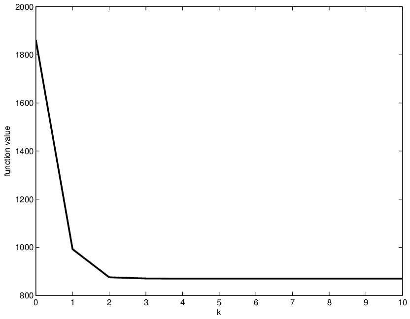
Consider the case where n=3n=3. The target sets are 55 square boxes with centers (−5,0,0)(-5,0,0), (1,4,4)(1,4,4), (0,5,0)(0,5,0), (−4,−3,2)(-4,-3,2) and (0,0,5)(0,0,5) and radii ri=1r_{i}=1 for i=1,…,5i=1,\ldots,5. Our results show that both Algorithm 4 and the subgradient method give an approximate SIB radius r∗≈3.18r_{*}\approx 3.18; see Figure 2.

Refer to caption
MATLAB RESULT
kk rkr_{k}
0 1861.36441
1 992.32230
2 875.27618
3 870.47714
4 869.94621
5 869.82005
6 869.79982
7 869.79676
8 869.79628
9 869.79621
10 869.79619
Figure 3: A smallest intersecting ball problem for cubes in high dimensions.
Example 5.3

Now we illustrate the performance of Algorithm 4 in high dimensions with the same setting in Example 5.2. We choose a modification of the pseudo random sequence from [31] with a0=7a_{0}=7 and for i=1,2,…i=1,2,\ldots

ai+1=mod​(445​ai+1,4096),bi=ai40.96.a_{i+1}=\textrm{mod}(445a_{i}+1,4096),\;\;b_{i}=\frac{a_{i}}{40.96}.

The radii rir_{i} and centers cic_{i} of the square boxes are successively set to b1,b2,…b_{1},b_{2},\ldots in the following order

10​r1,c1​(1),…,c1​(n);10​r2,c2​(1),…,c2​(n);…;10​rm,cm​(1),…,cm​(n).10r_{1},c_{1}(1),\ldots,c_{1}(n);10r_{2},c_{2}(1),\ldots,c_{2}(n);\ldots;10r_{m},c_{m}(1),\ldots,c_{m}(n).

Consider m=100,n=1000m=100,n=1000. Figure 3 shows the approximate values of the radii rkr_{k} for k=0,…,10k=0,\ldots,10.

Refer to caption
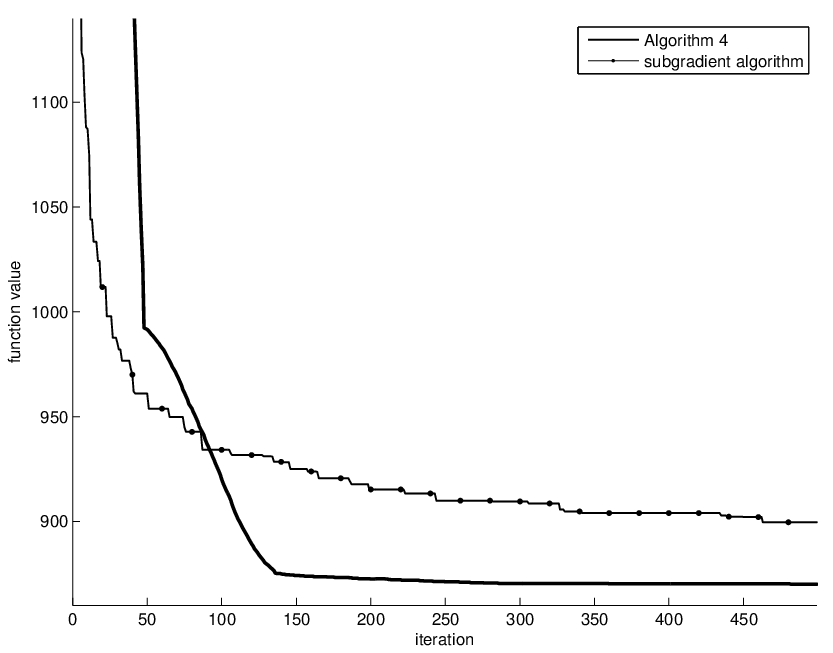
Figure 4: Comparison between minimization majorization algorithm and subgradient algorithm.

We also implement algorithm 4 in comparison with the subgradient algorithm. From our numerical results, we see that Algorithm 4 performs much better than the subgradient algorithm in both accuracy and speed. In the case where the number of target sets is large or the dimension mm is high, the subgradient algorithm seems to be stagnated but Algorithm 4 still performs well. Figure 4 shows that comparison between Algorithm 4 and the subgradient algorithm. Note that in Algorithm 4, we count every iteration of Nesterov’s accelerated gradient method in the total iteration count along the horizontal axis. Thus the “sharp corner” that can be seen at 50 iterations represents the transition form x0x_{0} to x1x_{1}, and a subsequent recalculation of pp by p=σ​pp=\sigma p.

6 Concluding Remarks

Based on the log-exponential smoothing technique and the minimization majorization algorithm, we have developed an effective numerical algorithm for solving the smallest intersecting ball problem. The problem under consideration not only generalizes the Sylvester smallest enclosing circle problem, but also opens up the possibility of applications to other problems of constrained optimization, especially those that appear frequently in machine learning. Our numerical examples show that the algorithm works well for the problem in high dimensions. Although a number of key convergence results are contained in this paper, our future work will further develop an understanding of the convergence rate of this algorithm

Acknowledgement. The author would like to thank Prof. Jie Sun for giving comments that help improve the presentation of the paper.

References

  • [1] J. Alonso, H. Martini, and M. Spirova, Minimal enclosing discs, circumcircles, and circumcenters in normed planes, Comput. Geom. 45 (2012), 258–274.
  • [2] D. Bertsekas, A. Nedic, and A. Ozdaglar, Convex Analysis and Optimization, Athena Scientific, Boston, 2003.
  • [3] S. Boyd and L. Vandenberghe, Convex Optimization, Cambridge University Press, Cambridge, England, 2004.
  • [4] D. Cheng, X. Hu, C. Martin, On the smallest enclosing balls, Commun. Inf. Syst. 6 (2006), 137–160.
  • [5] E. Chi, H. Zhou, K. Lange, Distance Majorization and Its Applications, Math Program., in press.
  • [6] L. Drager, J. Lee, C. Martin, On the geometry of the smallest circle enclosing a finite set of points, J. Franklin Inst. 344 (2007), 929–940.
  • [7] K. Fischer and B. Gartner, The smallest enclosing ball of balls: Combinatorial structure and algorithms, Comput. Geom. 14 ( 2004), 341–-378.
  • [8] S. K. Jacobsen, An algorithm for the minimax Weber problem, European J. Oper. Res. 6 (1981), 144–148.
  • [9] D. W. Hearn and J. Vijay, Efficient algorithms for the (weighted) minimum circle problem, Oper. Res. 30 (1981), 777–-795.
  • [10] J. B. Hiriart-Urruty and C. Lemaréchal, Funndamental of Convex Analysis, Springer-Verlag, 2001.
  • [11] D.R. Hunter, K. Lange, Tutorial on MM algorithms. Amer Statistician 58( 2004), 30–37.
  • [12] K. Lange, D. R. Hunter, I. Yang, Optimization transfer using surrogate objective functions (with discussion). J Comput Graphical Statatisctis 9 (2000), 1–59.
  • [13] J. Mairal. Incremental majorization-minimization optimization with application to large-scale machine learning. arXiv preprint arXiv:1402.4419 (2014).
  • [14] N. M. Nam, N. T. An, R. B. Rector and J. Sun, Nonsmooth algorithms and Nesterov’s smoothing technique for generalized Fermat-Torricelli problems. SIAM J. Optim. 24 (2014), no. 4, 1815–1839.
  • [15] B. S. Mordukhovich and N. M. Nam, An Easy Path to Convex Analysis and Applications, Morgan & Claypool Publishers, 2014.
  • [16] N. M. Nam and N. Hoang, A generalized Sylvester problem and a generalized Fermat-Torricelli problem, to appear in Journal of Convex Analysis.
  • [17] N. M. Nam, N. T. An and J. Salinas, Applications of convex analysis to the smallest intersecting ball problem, J. Convex Anal. 19 (2012), 497–518.
  • [18] Yu. Nesterov, Smooth minimization of non-smooth functions, Math. Program. 103 (2005), 127–152.
  • [19] Yu. Nesterov, Introductory lectures on convex optimization. A basic course. Applied Optimization, 87. Kluwer Academic Publishers, Boston, MA, 2004.
  • [20] Yu. Nesterov, A method for unconstrained convex minimization problem with the rate of convergence O(1k2\frac{1}{k^{2}}). Doklady AN SSSR (translated as Soviet Math. Docl.) 269(1983), 543–547.
  • [21] F. Nielsen and R. Nock, Approximating smallest enclosing balls with applications to machine learning, Internat. J. Comput. Geom. Appl. 19 (2009), 389–414.
  • [22] R. T. Rockafellar, Convex Analysis, Princeton University Press, Princeton, NJ, 1970.
  • [23] A. Saha, S. Vishwanathan, and X. Zhang, Efficient approximation algorithms for minimum enclosing convex shapes, proceedings of SODA, 2011.
  • [24] J. J. Sylvester, A question in the geometry of situation. Quarterly Journal of Pure and Applied Mathematics 1:79(1857).
  • [25] E. Welzl, Smallest enclosing disks (balls ellipsoids). H. Maurer, editor, Lecture Notes in Comput. Sci. 555 (1991), 359–370.
  • [26] S. Xu, R. M. Freund, and J. Sun, Solution methodologies for the smallest enclosing circle problem. A tribute to Elijah (Lucien) Polak. Comput. Optim. Appl. 25(2003), no. 1-3, 283–292.
  • [27] E. A. Yildirim, On the minimum volume covering ellipsoid of ellipsoids, SIAM J. Optim. 17 (2006), 621–641.
  • [28] E. A. Yildirim, Two algorithms for the minimum enclosing ball problem, SIAM J. Optim. 19 (2008), 1368–1391.
  • [29] X. Zhai, Two problems in convex conic optimization, master’s thesis, National University of Singapore, 2007.
  • [30] T. Zhou, D. Tao, and X. Wu, NESVM: a Fast Gradient Method for Support Vector Machines, IEEE International Conference on Data Mining (ICDM), 2010.
  • [31] G. Zhou, K. C. Toh, and J. Sun, Efficient algorithms for the smallest enclosing ball problem, Comput. Optim. Appl. 30 (2005), 147–160.