Role of the phase-matching condition in non-degenerate four-wave mixing in hot vapors for the generation of squeezed states of light
Abstract
Non-degenerate forward four-wave mixing in hot atomic vapors has been shown to produce strong quantum correlations between twin beams of light [McCormick et al, Opt. Lett. 32, 178 (2007)], in a configuration which minimizes losses by absorption. In this paper, we look at the role of the phase-matching condition in the trade-off that occurs between the efficiency of the nonlinear process and the absorption of the twin beams. To this effect, we develop a semi-classical model by deriving the atomic susceptibilities in the relevant double-lambda configuration and by solving the classical propagation of the twin-beam fields for parameters close to those found in typical experiments. These theoretical results are confirmed by a simple experimental study of the nonlinear gain experienced by the twin beams as a function of the phase mismatch. The model shows that the amount of phase mismatch is key to the realization of the physical conditions in which the absorption of the twin beams is minimized while the cross-coupling between the twin beams is maintained at the level required for the generation of strong quantum correlations. The optimum is reached when the four-wave mixing process is not fully phase matched.
pacs
42.50.Gy,42.65.Yj,42.65.HwI Introduction
Continuous-variable entanglement can be generated deterministically with a phase-insensitive optical amplifier. For a gain larger than 1, the system produces a two-mode squeezed state where the signal and the idler (here referred to as probe and conjugate respectively) display EPR-type entanglement [1]. Such an amplifier can be realized using a nonlinear optical process such as parametric down-conversion [2, 3] or four-wave mixing (4WM) [4]. In real physical systems, the presence of absorption reduces the amount of quantum correlations which can be generated, and although 4WM in atomic vapors can lead to large gains, resonant atomic processes are also responsible for losses, which limit the amount of observable squeezing. Recently, a configuration in 4WM was found which reduces absorption [5, 6, *lukin_resonant_2000], and generates large degrees of squeezing [8, 9, 10, 11].
There have been a number of reasons put forward to explain this success. The main one is the nature of the nonlinearly, which is based on coherence effects between the hyperfine electronic ground states rather than on the saturation of a transition of a two-level atom [12, 6, *lukin_resonant_2000]. Indeed, avoiding a large atomic population in the excited state is key to the reduction of the noise associated with spontaneous emission. More specifically, it was pointed out that the D1 line of alkali atoms is particularly amenable to the establishment of a ground state coherence [13]. We show here that the production of squeezing is also due in great part to a judicious choice of the parameters that most greatly influence the phase-matching condition of the nonlinear process, specifically the relative frequencies of the beams and the angle between the beams. Maybe surprisingly, the highest levels of squeezing are achieved when the system is not fully phase matched.
The paper is divided as follows. In section II, we theoretically study 4WM in an atomic vapor in a double-lambda configuration where both pumps are detuned from the atomic resonance. From the atomic susceptibilities we evaluate the impact of the phase-matching condition on the gain and the absorption in the forward-4WM configuration. In section III, we report on a systematic experimental study of the phase-matching condition which confirms the findings of section II. In section IV, we extend our model to take into account the Doppler effect due to the thermal motion of the atoms. Finally in section V we discuss the impact of our theoretical and experimental findings on the possibility of generating strong two-mode squeezing with 4WM in a hot vapor. From the model we deduce the best parameters in terms of beam geometry and beam detunings, and compare them to the recent squeezing experiments of Refs. 8, 9, 10, 11.
II Theoretical model of non-degenerate four-wave mixing
When describing nonlinear media in the presence of off-resonant fields, it is common to separate the response of the system into a linear part and a nonlinear part [14]. The linear contribution leads to an index of refraction which modifies the linear dispersion relation for each of the individual light fields in the medium. The nonlinear part acts as a perturbative source term in the propagation equations. It enables energy transfer between light fields for those configurations where the phase-matching condition is fulfilled, that is to say when the total wave-vector of the waves giving up energy equals the total wave-vector of the waves receiving the energy. The relevant wave-vectors are those in the medium. They are equal to the wave-vectors in vacuum times their corresponding indices of refraction.
In resonant media, such as atomic vapors excited close to atomic transitions, the medium is strongly perturbed by the presence of the light. For instance, optical pumping by a strong pump beam can affect the atomic populations in the hyperfine levels, leading to a strong change in the index of refraction seen by a weaker beam. In this case, the usual expansion separating the linear and the nonlinear responses may not be appropriate. Instead we consider an expansion of the nonlinear polarization to first order in the electric fields of the weak beams and to all orders in the electric fields of the pump beams [6, *lukin_resonant_2000].
We consider the double-lambda configuration, shown in Fig. 1, which was used to demonstrate intensity-difference squeezing and quadrature entanglement in a vapor of 85Rb [15, 16]. A non-degenerate 4WM parametric process drives an atom from one of the hyperfine ground states to the other hyperfine ground state and back to the initial state. In the process, two pump photons are converted into two twin photons, called probe and conjugate, with wave-vectors and in vacuum, and frequencies and . The non-linearity originates in a strong coupling between the probe and the conjugate fields mediated by the coherence of the electronic ground states [12]. Following the usual experimental configuration, we further assume that the two pump photons come from a single field, of wave-vector in vacuum and frequency . We denote the two-photon detuning of the pump and the probe: where is the hyperfine splitting of the ground state. The natural linewidth of the excited state is MHz. In the rest of the paper, we vary by changing the frequency of the probe. The 4WM resonance occurs roughly at (more on this below).
For simplicity, we assume that the coupling strengths of the pump to both transitions are equal, corresponding to a resonant Rabi frequency . Following Ref. 6, *lukin_resonant_2000, we calculate the atomic susceptibilities at the probe and conjugate frequencies in the limit of weak probe and conjugate fields. The detailed calculation is developed in the appendix. The susceptibilities are derived by calculating the steady-state value of the density matrix of a 4-level system interacting with the four fields of the double lambda. The atomic polarization at the frequencies of the probe and the conjugate is proportional to the average oscillating atomic electric dipole at those frequencies and therefore to the off-diagonal components of the density matrix corresponding to these transitions. To first order in the probe and conjugate fields, the atomic polarization is described by two direct susceptibilities, and , and two cross-susceptibilities, and , given by Eqs. (20–23). The cross-susceptibilities are responsible for the 4WM.
The propagation equations for the slowly varying envelopes of the probe and conjugate fields and , using the polarization expressions (18) and (19), are given in steady state by:
| (1) | |||||
| (2) |
Furthermore, if we consider the case of co-propagating, or nearly co-propagating, beams along the axis, these equations read:
| (3) | |||||
| (4) |
where is the projection of the geometric phase-mismatch on the axis, and the conservation of energy imposes the condition .
In the low pump depletion limit, which is usually experimentally the case, the pump Rabi frequency is constant along the vapor cell and these equations are simply first order coupled linear differential equations. When the dynamics is dominated by the cross-terms and no conjugate field is injected, the probe and conjugate fields grow asymptotically exponentially and the system behaves like a phase-insensitive amplifier for a probe input field [14, 17]. At the quantum level, these cross-terms are responsible for the creation of quantum correlations between the output probe and conjugate fields, leading to the production of a two-mode squeezed state [1, 16]. The larger the gain of the amplifier, the greater the amount of squeezing.
The full dynamics is more complicated than pure 4WM because of the presence of the direct terms and . However the general form of Eqs. (3) and (4) offers us a straightforward interpretation of and in terms of effective linear susceptibilities for the probe and the conjugate fields. Note that unlike the usual linear susceptibilities, these effective susceptibilities depend, nonlinearly, on the pump field. Therefore they give rise to a pump-dependent complex index of refraction for the probe and the conjugate. The real part influences the phase-matching of the process, as discussed below. The imaginary part translates into absorption.
In the original proposal by Lukin et al [6, *lukin_resonant_2000], the pump beams are resonant with an atomic transition (). This results in a remarkable situation where the pumps and the twin beams fulfill the two-photon Raman resonance and enter an electromagnetically-induced transparency (EIT) condition [18]. As a result, they see a perfectly transparent medium, as witnessed by a vanishing imaginary part of and . At the same time, the cross-susceptibilities are enhanced by the coherence of the hyperfine electronic ground states. In theory, it should lead to very efficient 4WM and virtually no absorption, even for a weak pump. In practice, the EIT effect in hot vapors is limited because the Doppler effect, the presence of multiple excited hyperfine levels, and the finite transit time of the atoms in the laser beams all act to increase the decoherence rate between the ground states. This causes residual absorption of the probe field and as a result, only low levels of squeezing have been observed in this configuration [19].
In contrast, most recent squeezing experiments in hot atomic vapors operate at large detuning , typically 0.5 to 1 GHz, and at larger pump power [15, 9, 10, 11]. In these conditions, the susceptibilities take a different form from the resonant case. This off-resonant form is depicted in Fig. 2, for typical experimental parameters.
The first important property of these susceptibilities is that the 4WM resonance is shifted from the bare two-photon resonance () by the light shift created by the more resonant pump, on the transition. For typical experimental parameters, the shift is of the order of . In the rest of the paper, we call “blue side” of the 4WM resonance the range of detunings for which the frequency of the probe is above the 4WM resonance. The other side of the 4WM resonance is the “red side” (see Fig. 2).
The second property is that the imaginary part of (dashed line) is maximum at the 4WM resonance, due to Raman absorption. It is therefore not a good place to observe 4WM because the medium is essentially opaque for the probe at this detuning. On the other hand, decays much faster than the magnitude of when moving away from resonance, therefore there is a range of on each side of the 4WM resonance where still exhibits a substantial magnitude while has almost completely vanished (see Fig. 3). These regions of the two-photon detuning are better places to observe quantum effects.
The third important property is the behavior of the real part of (solid line), which is effectively responsible for the index of refraction for the probe. Around the 4WM resonance, is the sum of a dispersive feature resulting from the 4WM coupling and the off-resonance negative susceptibility resulting from the one-photon transition between ground state and excited state. These competing terms lead to a cancellation of around the bare two-photon resonance ().
It is legitimate to wonder if it would not be possible to take advantage of the coherence between the ground states to reduce the probe absorption through the EIT phenomenon, as envisioned in the original proposal. Theoretically, for a very low value of the ground state decoherence rate , it is indeed possible to observe the transparency window at the bare two-photon resonance, as shown in Fig. 3. In practice, such low decoherence rates are not achieved due to imperfections associated with hot vapors. Experimental results reported below and in Refs 20, 21 are compatible with a higher value , for which there is no marked transparency window. In spite of the lack of efficient EIT, the off-resonant value of is small enough compared to the cross-coupling to ensure efficient 4WM, and experimental set-ups do not require special precautions with regards to decoherence sources such as stray magnetic fields.
Note that these considerations do not apply to the conjugate field, which is much further detuned from resonance than the probe. The direct susceptibility of the conjugate is substantially smaller than the other susceptibilities and can be regarded as zero in practice.
Now that adequate ranges of have been identified for which probe losses are negligible compared to 4WM amplification, the question is whether there is a geometric configuration of the light fields for which 4WM is phase matched. To answer this question, we recall from Ref. 6, *lukin_resonant_2000 the solutions to the propagation equations (3) and (4), for a seed on the input probe and no input conjugate:
| (5) | |||||
| (6) |
where is the length of the medium, , , , , , and . We define the probe and conjugate intensity gains and as and .
From these expressions, we plot in Fig. 4 the probe and conjugate gains as a function of and the geometric phase mismatch . One can see that for , the maximum gain is obtained around , for both the probe and the conjugate. When increases, the gain on both the probe and the conjugate increases while the gain resonance moves towards the 4WM resonance (shown with the vertical dashed line). At larger , the gain resonance comes asymptotically within of the 4WM resonance, the probe intensity drops while the conjugate intensity keeps increasing. Finally, at large , the conjugate intensity also drops.
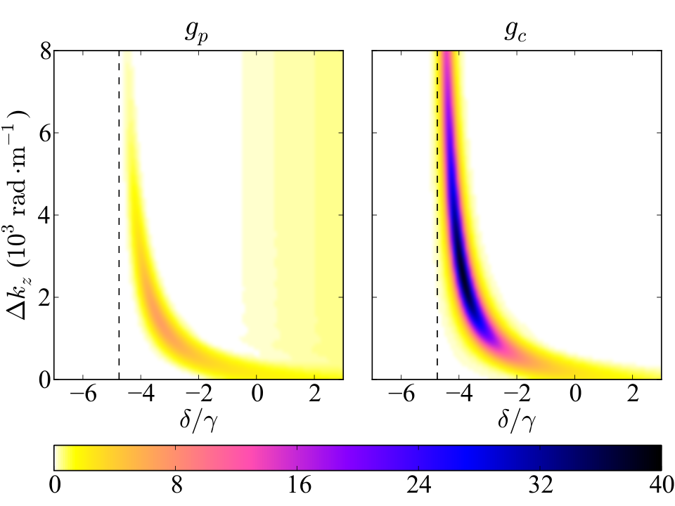
The position of the gain resonance is the result of the 4WM phase-matching (or absence thereof), and is influenced by the effective index of refraction seen by the probe and the conjugate as follows. Since is much smaller than the other susceptibilities, the conjugate effectively propagates in a medium of index 1. The situation is different for the probe, for which the index of refraction changes sign at the 4WM resonance and at , as indicated in Fig. 2. The change in sign of at means that the probe experiences an effective index of refraction, , smaller than 1 for and larger than 1 between and the 4WM resonance. We assume that the index of refraction experienced by the pump, , is close to 1 since the pump tends to optically pump the atoms towards the ground state of the off-resonant transition . This assumption will be refined later.
The geometric phase-matching condition is the phase-matching condition in free space. It is fulfilled only when the beams are rigorously co-propagating, as shown in Fig. 5(a). For the process to be efficient, the effective phase-matching condition must be fulfilled:
| (7) |
as shown in Fig. 5(b). This condition is identical to the geometric phase-matching condition () only when , which occurs around (Fig. 2). When , the effective phase-matching condition (7) imposes , which corresponds to having a finite angle between the pump and the probe and conjugate 11 1 As the angle between the pump and the probe, , is small and is close to 1, the angle between the pump and the conjugate is very close to .. This occurs on the red side of the 4WM resonance, for (see Fig. 2). As increases, the gain resonance is shifted towards higher values of and therefore towards the 4WM resonance. A negative geometric phase mismatch cannot be fulfilled. For this reason, no effective phase matching can happen on the blue side of the 4WM resonance, where .
Close to the 4WM resonance, the increase in accounts for the reduction in probe power with respect to the conjugate power, seen in Fig. 4. In this region, a high level of probe absorption coupled to a large 4WM gain still produces a strong conjugate output. At larger angle , the effective phase-matching condition requires a value of so close to the 4WM resonance that the high probe loss prevents the 4WM from happening at all.
III Experimental verification
In order to verify the theoretical predictions, a test was performed, as shown in Fig. 6 in which a mW pump laser of beam waist mm drives the D1 line at 795 nm in a 12-mm-long cell of 85Rb vapor, heated and temperature stabilized at C. A seed beam at the probe frequency is produced by diverting a fraction of the pump through an AOM operating at GHz in a double-pass arrangement. This seed beam, of power W and waist mm, then intersects with the pump inside the cell at a small angle . The probe and conjugate beams are perpendicularly polarized with respect to the pump which is rejected at the output with a polarizing beam splitter. From the measured input seed power , output probe power , and output conjugate power , the probe and conjugate gains ( and , respectively) are obtained.

A dichroic-atomic-vapor laser lock [23] is in place to regulate the pump frequency thus maintaining a constant . The angle of intersection between the pump and probe is set by manually adjusting a pair of input mirrors, and is adjusted by changing the AOM drive frequency. For a selection of values of , is swept over a range of typically MHz, where noticeable gains and are observed. The angular range used, from 0∘ to 1∘, satisfies the condition that there must be a full overlap of the beams over the cell length (this is achievable for up to ). Figures 7(a, b) show the contour plots of and as a function of and .
The general features of figure 4 are reproduced, including the shift of the gain peaks towards the 4WM resonance when is increased, as well as the crossover between probe power and conjugate power. The crossover is the value of for which the peak conjugate power is equal to the peak probe power. The main discrepancy between the experimental data and the theoretical prediction is the measured drop in probe and conjugate power for . This leads to peak gains for both the probe and the conjugate which are well below the theoretical prediction. There are two main reasons for this behavior. Firstly, for a finite , the Doppler effect due to the thermal motion of the atoms does not cancel between the pump and the twin beams. For , the residual Doppler effect on reaches , which is roughly the width of the gain peak itself. This results in a broadening of the gain resonance at larger angles , when compared to the resonance given by the theoretical model, which is visible in Fig. 7.
Secondly, and perhaps more importantly, when is increased past 0.5∘, the probe beam is subject to a strong effective cross-Kerr interaction with the pump around the gain resonance. This is due to the fact that as the gain peak moves closer to the 4WM resonance the effective index of the probe is resonantly enhanced, as shown by the behavior of in Fig. 2. As a result, the transverse intensity variation of the pump realizes a strong lens for the probe, causing it to emerge from the cell with an angle of divergence comparable to or larger than itself 22 2 The full Kerr action of the pump on the probe is the compound effect of the change of magnitude of the index of refraction at resonance and the frequency shift of the resonance due to the light shift caused by the pump..
The good agreement between the theoretical model and the measurements at angles where the probe focusing is negligible gives us the opportunity to extract the values of those parameters which are not otherwise easily obtained, in particular the pump Rabi frequency , the atom density , and most importantly the decoherence rate . Moreover, as explained in the appendix, we can also introduce the effect of the index of refraction of the pump on the phase-matching condition by replacing the geometric phase mismatch with , where is the pump index of refraction. By fitting the model on the data, as shown in Figs. 7(c, d), we find that , , , and . For this data set, the pump detuning was determined to be by calibrating the position of the 4WM gain against a Rb spectroscopy spectrum. As expected, the index of refraction for the pump on the blue side of the atomic resonance is smaller than one.
One can check that the parameters extracted from the fit are broadly consistent with the estimated experimental conditions. Our pump beam parameters lead to a peak intensity of , which results in a resonant Rabi frequency for a mean electric dipole [25]. From the vapor pressure data summarized in Ref. 25, the number density of 85Rb at C is . Finally the index of refraction for the pump, evaluated for ground state populations of 6% in the lower hyperfine state and 94% in the upper hyperfine state, as given by Eqs. (24–27), and for the electric dipole value given above, is .
IV Doppler broadening
The model developed above does not take into account the Doppler broadening caused by the thermal motion of the atoms in the cell. The good agreement between the model and the experimental data suggests that considering only average values of the single-photon detunings and captures most of the physics at play. However, considering that the probe is typically tuned to the edge of the Doppler profile, it is legitimate to wonder what level of absorption this causes. It turns out that although the EIT has a limited impact, the pump field is highly saturating at resonance and causes a wide Autler-Townes splitting for those atoms resonant with the probe field. This renders even the resonant part of the atomic vapor highly transparent for the probe as long as the optical depth is not too large. In practice, noticeable levels of squeezing can be observed for as low as 500 MHz [8], which is well inside the Doppler profile at our operational temperature.
In order to verify these assumptions, we extended the above model to include the full Doppler distribution of detunings. The result, fitted to the gain curve of the probe as a function of , is shown in Fig. 8. The small discrepancy in the width of the single-photon resonance is due to the fact that the model does not include the hyperfine structure of the excited state, whose main effect is to broaden the apparent Doppler profile.
V Optimizing for quantum noise reduction
The observation of large levels of intensity-difference quantum noise reduction requires a near-perfect phase-insensitive amplifier with a gain of at least a few units. In the case of 4WM in a hot atomic vapor, this means that the absorption of the twin beams must be kept to a minimum while ensuring that efficient 4WM can take place. As pointed out previously, the two-photon detuning which fulfills those two conditions is , and not the 4WM resonance in itself. This is firstly because away from the 4WM resonance the probe susceptibility responsible for the absorption drops faster than the cross-susceptibility responsible for the 4WM gain, and secondly because the ground state coherence reduces the probe absorption at that detuning 33 3 It is not exactly due to the light shift created by the pump beam on the transition..
From the previous discussion, at a detuning , effective phase matching of the 4WM process requires geometric phase-matching . When corrected for the index of refraction for the pump, this condition corresponds to the introduction of a small angle between the pump and the probe beams. This is indeed how the best levels of squeezing have been experimentally observed [8, 9, 10, 11]. The production of squeezed light by non-degenerate 4WM in a hot vapor therefore benefits from two favorable circumstances. First, the optimum angle is small enough that the residual Doppler effect acting on the nearly co-propagating beams is much smaller than the width of the gain peak. Second, the same angle is large enough that the beams participating in the 4WM can be spatially separated at the output of the vapor cell.
It is worth noting that in certain conditions, a small amount of loss on the probe beam can be beneficial. For instance, for a probe seed containing a large amount of classical noise, it is useful to have twin beams of equal powers in order to ensure proper rejection of the classical noise in the balanced detection [8]44 4 We consider here only the case where the detector is perfectly balanced, with equal electronic gains on both inputs.. In particular, the existence of points in the parameter space where the probe and conjugate powers are perfectly balanced has allowed the detection of 8 dB of intensity-difference squeezing at frequencies as low as 2.5 kHz, despite the presence of substantial technical noise on the input probe [8].
Conclusion
We have shown that it is possible to phase-match 4WM in a hot atomic vapor so that absorption is reduced to a level where quantum effects could manifest themselves. Most reports of large squeezing generated by non-degenerate forward 4WM in hot vapors to date have indeed used a similar arrangement as the one presented here, with nearly identical atomic and beam parameters. Furthermore, the model we have developed appears very accurate for small angles between beams, even in its simple form neglecting both the Doppler effect and the Zeeman sub-structure. It allows the robust extraction of parameters which would be difficult to determine by direct measurement, such as the decoherence rate of the ground states.
By providing further insight into the mechanism of the process, the present results may lead to the realization of different configurations or different regimes amenable to the production of interesting quantum states of light, such as multi-spatial-mode phase-sensitive amplifiers [28, *corzo_noiseless_2012].
We acknowledge useful discussions with Colin McCormick, Ennio Arimondo and Paul Lett, and we thank Etienne Pertreux for his help in the early stages of this project. This research was supported by the Engineering and Physical Sciences Research Council grants EP/E036473/1 and EP/I001743/1.
*
Appendix A Expressions for the susceptibilities
A.1 Derivation of the susceptibilities for the probe and the conjugate
In this appendix we derive the dynamics of the double-lambda configuration described in the paper. The response of an atomic system to an optical field is determined by the polarization of the medium, which acts as the driving term in the wave equation. For a medium that consists of non-interacting particles, such as a dilute atomic vapor, the polarization of the medium is of the form [14]
where is the number density of the atomic medium and is the atomic dipole moment operator. The polarization of the medium can be written in terms of the atomic eigenstates, such that it takes the form
where the sum is over all the involved atomic transitions, is the frequency of the field that couples the transition between levels and , is the density matrix element between levels and in a rotating frame at frequency , and is the dipole matrix element between levels and . For an isotropic medium, the polarization of the atomic medium at a particular frequency is given by
Thus, the response is completely determined by the atomic coherence of the corresponding transition.
The equations of motion for the density matrix elements in the rotating frame can be shown to be of the form [14]
where is the detuning of the field at frequency from the transition between levels and , is the population decay rate from level to level , is the dipole dephasing rate, is the total decay rate out of level , and is the dipole dephasing rate due to any other source of decoherence.
We now specialize to our 4WM process in the double-lambda configuration, shown in Figs. 1 and 9, with a single pump field, . For this case the total electric field is of the form
where , , and are the field amplitudes for the pump, the probe, and the conjugate, respectively, and are unit vectors describing the polarization of the fields. We assume that the pump couples the transitions and , the probe couples transition , the conjugate couples transition , and that the transitions and are not dipole allowed. With these assumptions and using the rotating-wave approximation, the equations of motion for the density matrix elements take the form
| (8) | |||||
| (9) | |||||
| (10) | |||||
| (11) | |||||
| (12) | |||||
| (13) | |||||
| (14) | |||||
| (15) | |||||
| (16) | |||||
| (17) |
where and give the Rabi frequencies for the two transitions coupled by the single pump, the Rabi frequency for the transition coupled by the probe, and the Rabi frequency for the transition coupled by the conjugate. In order to completely eliminate the explicit time dependence when doing the rotating-wave approximation, the frequencies of the pump, probe, and conjugate fields need to satisfy the relation
which is just an energy conservation condition for the 4WM process.
In order to solve the above equations and obtain analytical expressions, we assume that the probe and conjugate fields are weak fields, such that we only keep terms to first order in and . In this case, the polarization of the medium at frequency (where indicates probe or conjugate frequency) can be divided into two different terms, one that is proportional to the field at frequency and one that is proportional the field at frequency , such that
| (18) | |||||
| (19) | |||||
In doing this, we have introduced the susceptibility of the atomic medium , which completely characterizes the response of the atomic system for a given field. The direct susceptibilities act as the effective linear susceptibilities for the probe and conjugate, respectively; the cross-susceptibilities are responsible for the 4WM process.
In addition to the approximations mentioned above, we assume the dipole moments for the two pump transitions to be equal, such that . Under these approximations we can solve the density matrix equations, Eqs. (8-17), to all orders in the pump field () and in steady-state condition for and to find that
| (20) | |||||
| (21) | |||||
| (22) | |||||
| (23) | |||||
where we have defined
the population differences
| (24) | |||
| (25) | |||
| (26) | |||
| (27) |
and the complex decay rates
In deriving these equations, we have assumed that the total decay rate out of the excited states are the same and with equal branching ratios to the two ground states; that is, and . In addition, we assume that the additional dipole dephasing term is only significant for the ground state coherence, such that and .
A.2 Index of refraction for the pump
In the above derivation of the susceptibilities for the probe and the conjugate, we have implicitly set , the amplitude for the pump electric field, to be a constant throughout the medium. This assumes that the pump is neither dephased or absorbed. In practice, the pump detuning is large enough to neglect absorption, but even a small index of refraction may have a substantial impact on the phase-matching condition of the 4WM process. The effect of refraction on the pump is to multiply (and therefore ) by a running phase factor as the pump propagates. This can be taken into account by simply replacing in by , where is the index of refraction. The index of refraction created by the population of the ground state can be estimated to be with
where is the dipole matrix element of the transition for large detunings and is the detuning, which is taken to be much larger than the hyperfine splitting of the excited state.
References
- [1] M. D. Reid, Phys. Rev. A 40, 913 (1989).
- [2] A. Heidmann, R. J. Horowicz, S. Reynaud, E. Giacobino, C. Fabre, and G. Camy, Phys. Rev. Lett. 59, 2555 (1987).
- [3] Z. Y. Ou, S. F. Pereira, H. J. Kimble, and K. C. Peng, Phys. Rev. Lett. 68, 3663 (1992).
- [4] C. Silberhorn, P. K. Lam, O. Weiß, F. König, N. Korolkova, and G. Leuchs, Phys. Rev. Lett. 86, 4267 (2001).
- [5] P. R. Hemmer, D. P. Katz, J. Donoghue, M. Cronin-Golomb, M. S. Shahriar, and P. Kumar, Opt. Lett. 20, 982 (1995).
- [6] M. D. Lukin, P. R. Hemmer, M. Löffler, and M. O. Scully, Phys. Rev. Lett. 81, 2675 (1998).
- [7] M. D. Lukin, P. R. Hemmer, and M. O. Scully, in Advances in Atomic Molecular, and Optical Physics, Vol. 42, edited by B. Bederson and H. Walther (Elsevier Academic Press Inc, San Diego, 2000) pp. 347–386.
- [8] C. F. McCormick, A. M. Marino, V. Boyer, and P. D. Lett, Phys. Rev. A 78, 043816 (2008).
- [9] Q. Glorieux, L. Guidoni, S. Guibal, J.-P. Likforman, and T. Coudreau, Phys. Rev. A 84, 053826 (2011).
- [10] M. Jasperse, L. D. Turner, and R. E. Scholten, Optics Express 19, 3765 (2011).
- [11] Z. Qin, J. Jing, J. Zhou, C. Liu, R. C. Pooser, Z. Zhou, and W. Zhang, Opt. Lett. 37, 3141 (2012).
- [12] M. D. Reid, D. F. Walls, and B. J. Dalton, Phys. Rev. Lett. 55, 1288 (1985).
- [13] R. C. Pooser, A. M. Marino, V. Boyer, K. M. Jones, and P. D. Lett, Optics express 17, 16722–16730 (2009a).
- [14] R. W. Boyd, Nonlinear Optics (Academic Press, 2008).
- [15] C. F. McCormick, V. Boyer, E. Arimondo, and P. D. Lett, Opt. Lett. 32, 178 (2007).
- [16] V. Boyer, A. M. Marino, R. C. Pooser, and P. D. Lett, Science 321, 544 (2008).
- [17] R. C. Pooser, A. M. Marino, V. Boyer, K. M. Jones, and P. D. Lett, Phys. Rev. Lett. 103, 010501 (2009b).
- [18] K.-J. Boller, A. Imamoglu, and S. E. Harris, Phys. Rev. Lett. 66, 2593 (1991).
- [19] C. H. van der Wal, M. D. Eisaman, A. André, R. L. Walsworth, D. F. Phillips, A. S. Zibrov, and M. D. Lukin, Science 301, 196 (2003).
- [20] V. Boyer, C. F. McCormick, E. Arimondo, and P. D. Lett, Phys. Rev. Lett. 99, 143601 (2007).
- [21] Q. Glorieux, R. Dubessy, S. Guibal, L. Guidoni, J.-P. Likforman, T. Coudreau, and E. Arimondo, Phys. Rev. A 82, 033819 (2010).
- [22] As the angle between the pump and the probe, , is small and is close to 1, the angle between the pump and the conjugate is very close to .
- [23] K. L. Corwin, Z.-T. Lu, C. F. Hand, R. J. Epstein, and C. E. Wieman, Applied Optics 37, 3295 (1998).
- [24] The full Kerr action of the pump on the probe is the compound effect of the change of magnitude of the index of refraction at resonance and the frequency shift of the resonance due to the light shift caused by the pump.
- [25] D. A. Steck, “Rubidium 85 D line data,” (2012), http://steck.us/alkalidata (revision 2.1.5).
- [26] It is not exactly due to the light shift created by the pump beam on the transition.
- [27] We consider here only the case where the detector is perfectly balanced, with equal electronic gains on both inputs.
- [28] N. Corzo, A. M. Marino, K. M. Jones, and P. D. Lett, Optics Express 19, 21358 (2011).
- [29] N. V. Corzo, A. M. Marino, K. M. Jones, and P. D. Lett, Phys. Rev. Lett. 109, 043602 (2012).