An effective gauge-Higgs operators analysis of new physics associated with the Higgs

We-Fu Chang Wei-Ping Pan Fanrong Xu Affiliation: Department of Physics, National Tsing Hua University, HsinChu 300, Taiwan Email: wfchang@phys.nthu.edu.tw Email: two.joker@gmail.com Email: frxu@phys.nthu.edu.tw Affiliation: E-mail: , ,

Abstract:

We study the new physics(NP) related to the recent discovered $125$ GeV Higgs by employing an important subset of the standard model(SM) gauge invariant dimension-six operators constructed by the the SM Higgs and gauge fields. Explicitly, we perform a model-independent study on the production and decays of the Higgs, the electric dipole moments(EDMs) of the neutron and the electron, and we take into account the anomalous magnetic dipole moments of muon and electron as well. We find that, even all Higgs decay channels agree with the SM predictions, the SM theoretical uncertainties provide a lot of room to host NP associated with the 125 GeV boson. A linear relation is revealed in our numerical study that $\mu_{ZZ}\simeq\mu_{WW}$ and $0.6\lesssim\mu_{ZZ,WW}\lesssim 1.4$ at $95\%$ CL with or without the EDMs constraints. The neutron and electron EDMs severely constrain the relevant Wilson coefficients. Therefore the CP violating components in the $h\rightarrow WW,ZZ$ channels are too small, $\sim{\cal O}(10^{-5})$ , to be detected at the LHC. However, we point out that even the parity of the 125GeV boson has been largely determined to be even in the $h\to ZZ$ channel, one should pay special attention to the potentially large CP violation in the $h\to\gamma\gamma$ and $h\to\gamma Z$ channels. This should be seriously checked in the future spin correlation experiments.

Keywords:

Higgs, Beyond Standard Model, CP violation

1 Introduction

The high energy physics community has been excited about the recent finding of a standard model(SM) like Higgs boson $h$ , the final piece of the SM we had long craved for, at the mass around 125 GeV at the LHC [1, 2]. So far, except the Higgs diphoton decay which is $\sim 1\sigma$ higher than its SM prediction, all other Higgs decay modes agree with the SM predictions within the experimental accuracies[13, 14, 15, 16, 17, 18, 19, 20, 3, 4, 5, 6, 7, 8, 9, 10, 11, 12]. The diphoton excess could be just the statistical fluctuation or due to some unknown systematic error, or it indicates the existence of new physics(NP) especially those connecting the Higgs and gauge sectors. Since last year, there have been many discussion and speculation about the diphoton excess, see for example[21]. Whether the diphoton excess is due to new physics or not will be settled down by more experimental efforts in the coming years. Although the statistics is still weak, the current Higgs decay data has already set some limits to the NP associated with the Higgs boson. On the other hand, we should also bear in mind that the uncertainty of the SM theoretical prediction for the Higgs productions range from $\sim 2\%$ for the vector boson fusion(VBF) to $\sim 15\%$ for the gluon-gluon fusion(GF)[22], the dominate Higgs production mechanism at the LHC, see Table 2. As for the decay branching ratios, the theoretical uncertainties range from $\sim 3\%$ for $h\rightarrow b{b}$ to $\sim 12\%$ for $h\rightarrow c\bar{c}$ [22], see Table 3. So even the experimental precision can be improved to reach a few percent level in the future, still, we will not be able to conclude the total absence of NP associated with the $\sim 125$ GeV boson. The interesting question will then be, “ How much room for new physics is still allowed due to the intrinsic SM theoretical uncertainty?” The main purpose of this paper is aiming for a model-independent constraint on the new physics associated with the Higgs based on the current and future data.

Meanwhile, the mass scale of exotic degrees of freedom(DOF) have been pushed to be greater than around $(0.4-8)$ TeV in various scenarios with different assumptions [23, 24]. Although a general analysis is lacking, it is now wildly believed that the cutoff scale, $\Lambda$ , for physics beyond SM begins to show up, should be much greater than the electroweak symmetry breaking scale, $v\sim 250$ GeV. Motivated by the diphoton excess and the exotic DOF(s) which is(are) heavier than the electroweak scale, it is reasonable to assume that the new physics effects can be captured and described by the dimension-six (dim-6) gauge-Higgs operators. We assume that the NP decouples at $\Lambda\gg v$ where the SM electroweak symmetry is not yet broken. Below the cutoff, there are only SM DOFs and the SM gauge symmetry are still honored by the low energy effective theory. The information and effects of NP are encoded in the form of the effective operators and their corresponding Wilson coefficients; see [25, 26] for the early general discussion. It is not new to study the Higgs physics by using the gauge-Higgs operators, see [27, 28, 29, 30, 31] for the previous studies along the same line and [32] for recent update including the Moriond 2013 data. However, some constraints have been over looked by those authors. The current analysis is so far the most comprehensive one to our best knowledge. We found those contributions which had been over looked indeed play a significant role to constrain NP.

In this work we should perform a model-independent analysis based on a subset of SM gauge invariant dim-6 gauge-Higgs operators. The presence of these dim-6 operators modified the gauge-Higgs couplings so as the Higgs decay and production at the tree-level. We should discuss the constraints on the relevant Wilson coefficients based on the LHC Higgs data and compare it to a benchmark case where all Higgs decay channels sit at the predicted SM values and the SM theoretical uncertainties are used as the experimental errors. We should show that indeed the parasitic NP can live comfortably within the SM theoretical uncertainties without much upsetting the global fit.

In addition to the tree-level processes, the coefficients of CP odd operators can be further constrained by estimating the loop-induced EDM at low energy. The apparent drawback of using effective operators is that we do not have a sensible prediction of the quantum effects at the loop level. The dim-6 gauge-Higgs operators do not close under the RG running[30]. To proceed, we consider the class of new physics in which the fermion EDM operators can be ignored at $\Lambda$ ¹¹ 1 This working assumption is also reasonable from phenomenology point of view. The current experimental limits require that the cutoff scale of these EDM operators to be greater than $10^{4}$ TeV if the corresponding Wilson coefficients are all $\sim{\cal O}(1)$ . Here we further assume the relevant Wilson coefficients for fermion EDMs generated by higher loops at $\Lambda$ or RG running are negligible. and the divergent part of loop integral be removed by the counter terms. Practically, we use dimensional regularization to calculate the leading contribution of CP-odd operator to the fermion EDM in the modified minimal subtraction ( $\overline{MS}$ ) scheme. Similarly, just for a ballpark estimation of how the $(g-2)$ will limit the NP, without any better argument, we also assume the charged lepton $(g-2)$ is negligible at $\Lambda$ . We calculate the loop induced muon and electron $(g-2)$ by using the gauge-Higgs operators at low energy and further constrain the relevant CP even Wilson coefficients. At the end, we will discuss a UV-complete toy model as an example for this assumption to work. But we should keep in mind that this assumption is not valid for the general case.

The paper is organized as follows. In section 2, we will lay out the important subset of the dim-6 gauge-Higgs operators. The needed Feynman rules for later calculation will be summarized there. The modifications to the Higgs decay and production due to these gauge-Higgs operators at the tree-level will be discussed in Section 3. The 1-loop contributions to EDM and g-2 will be given in Section 4. In Section 5, we present the numerical results and some remarks from the global fitting. In section 6, we briefly discuss how a degenerate solution can be resolved by the Higgs pair production cross section. As an example of the UV origin of the gauge-Higgs operators and to illustrate in what condition our analysis is valid, two simple models with scalar color octet, but in different $SU(2)$ representations, will be discussed. A brief summary will be given there as well. Finally, some technical details will be collected in Appendix.

2 Effective Lagrangian

As discussed in previous section, we assume that the NP associated with the SM Higgs production and decay could be largely captured and described by a set of $SU(3)_{C}\times SU(2)_{L}\times U(1)_{Y}$ invariant dim-6 gauge-Higgs effective operators and their Wilson coefficients[33, 28]

\mathscr{L}_{NP}=\sum_{i}(c_{i}\mathcal{O}_{i}+\tilde{c}_{i}\tilde{\mathcal{O}}_{i})\;\;\;(\mbox{i=1, 2, 12, 3})\,.

(1)

The relevant effective gauge-Higgs operators are

		$\displaystyle\mathcal{O}_{1}=\frac{g_{1}^{2}}{2\Lambda^{2}}H^{\dagger}HB_{\mu\nu}B^{\mu\nu},~~\tilde{\mathcal{O}}_{1}=\frac{g_{1}^{2}}{2\Lambda^{2}}H^{\dagger}HB_{\mu\nu}\widetilde{B}^{\mu\nu}\,,$
		$\displaystyle\mathcal{O}_{2}=\frac{g_{2}^{2}}{2\Lambda^{2}}H^{\dagger}HW^{a}_{\mu\nu}W^{a\,\mu\nu},~~\tilde{\mathcal{O}}_{2}=\frac{g_{2}^{2}}{2\Lambda^{2}}H^{\dagger}HW^{a}_{\mu\nu}\widetilde{W}^{a\,\mu\nu}\,,$
		$\displaystyle\mathcal{O}_{12}=\frac{g_{1}g_{2}}{2\Lambda^{2}}H^{\dagger}\tau^{a}HB_{\mu\nu}{W}^{a\,\mu\nu},~~\tilde{\mathcal{O}}_{12}=\frac{g_{1}g_{2}}{2\Lambda^{2}}H^{\dagger}\tau^{a}HB_{\mu\nu}\widetilde{W}^{a\,\mu\nu}\,,$
		$\displaystyle\mathcal{O}_{3}=\frac{g_{3}^{2}}{2\Lambda^{2}}H^{\dagger}HG_{\mu\nu}^{A}G^{A\,\mu\nu},~~\tilde{\mathcal{O}}_{3}=\frac{g_{3}^{2}}{2\Lambda^{2}}H^{\dagger}HG^{A}_{\mu\nu}\widetilde{G}^{A\,\mu\nu}\,,$		(2)

where the dual field strength tensor is defined as $\widetilde{F}_{\mu\nu}=\frac{1}{2}\epsilon_{\mu\nu\lambda\sigma}F^{\lambda\sigma}$ , $(F=B,W,G)$ , and the others are in the standard notations. Note that we have absorbed the SM gauge couplings and the cutoff $\Lambda$ into the definition of the operators. The operator ${\cal O}_{12}$ gives the direct $SU(2)$ - $U(1)_{Y}$ gauge mixing and modifies the oblique parameter $S$ [34] at the tree level[33]

\triangle S=\frac{8\pi v^{2}}{\Lambda^{2}}c_{12}\,,

(3)

when the two Higgs fields are replaced by their VEVs. The current $S$ parameter bound, $S=0.00^{+0.11}_{-0.10}$ [35], already sets a strong limit on $c_{12}$ . Similarly, the $\tilde{\mathcal{O}}_{3}$ operator yields an effective QCD $\theta_{QCD}$ -term and thus $\tilde{c}_{3}$ is strongly constrained by the neutron EDM. Therefore, we will set $c_{12}=\tilde{c}_{3}=0$ in our global analysis which will be discussed in the numerical section.

There are three more dim-6 gauge-Higgs operators which give rise to the tree-level modification to the coupling between Higgs and gauge fields:

(D_{\mu}H)^{\dagger}(D_{\nu}H)B^{\mu\nu}\,,\;(D^{\mu}H)^{\dagger}\sigma^{a}(D^{\nu}H)W^{a}_{\mu\nu}\,,\;|H^{\dagger}D_{\nu}H|^{2}\,.

(4)

However, these operators are severely constrained by electroweak precision tests; for example, the SM gauge boson mass matrix will be altered by these operators at tree-level. Since we are focusing on the Higgs physics at the LHC and it is safe to ignore these operators, we confine our analysis with six out of the eight gauge-Higgs operators given in Eq.(2).

Table 1: Feynman rules for the

hV^{\mu}(k_{1})V^{\prime\nu}(k_{2})

vertices, where

(k_{1},k_{2})

are entering the vertices.

\begin{array}[]{c|c|c}\hline\cr&S^{\mu\nu}(k_{1},k_{2})&P^{\mu\nu}(k_{1},k_{2})\\ \hline\cr\hline\cr h\gamma\gamma&i\,\frac{2vg_{2}^{2}s_{W}^{2}}{\Lambda^{2}}a_{1}&i\,\frac{2vg_{2}^{2}s_{W}^{2}}{\Lambda^{2}}\tilde{a}_{1}\\ h\gamma Z&i\,\frac{vg_{2}^{2}}{\Lambda^{2}}a_{2}&i\,\frac{vg^{2}_{2}}{\Lambda^{2}}\tilde{a}_{2}\\ hgg&i\,\frac{2vg_{3}^{2}}{\Lambda^{2}}c_{3}&i\,\frac{2vg_{3}^{2}}{\Lambda^{2}}\tilde{c}_{3}\simeq 0\\ hZZ&i\,\frac{2vg_{2}^{2}}{\Lambda^{2}}a_{4}&i\,\frac{2vg_{2}^{2}}{\Lambda^{2}}\tilde{a}_{4}\\ hWW&i\,\frac{2vg_{2}^{2}}{\Lambda^{2}}c_{2}&i\,\frac{2vg_{2}^{2}}{\Lambda^{2}}\tilde{c}_{2}\\ \hline\cr\end{array}

The relevant $hV^{\mu}(k_{1})V^{\prime\nu}(k_{2})$ Feynman rules are summarized in Table 1 where $(k_{1},k_{2})$ are the 4-momentum carried by the gauge bosons, and $(\mu,\nu)$ are the corresponding Lorentz indices. The two gauge invariant form factors are defined as

S^{\mu\nu}(k_{1},k_{2})=k_{2}^{\mu}k_{1}^{\nu}-k_{1}\cdot k_{2}g^{\mu\nu}\,,\;P^{\mu\nu}(k_{1},k_{2})=\epsilon^{\alpha\beta\mu\nu}k_{1\alpha}k_{2\beta}\,.

(5)

Also we define

		$\displaystyle a_{1}\equiv c_{1}+c_{2}-c_{12}\simeq c_{1}+c_{2}\,,\;\tilde{a}_{1}\equiv\tilde{c}_{1}+\tilde{c}_{2}-\tilde{c}_{12}\,,$
		$\displaystyle a_{2}\equiv s_{2W}\left(c_{2}-c_{1}t_{W}^{2}-\frac{1}{2}c_{12}(1-t_{W}^{2})\right)\simeq s_{2W}\left(c_{2}-c_{1}t_{W}^{2}\right)\,,$
		$\displaystyle\tilde{a}_{2}\equiv s_{2W}\left(\tilde{c}_{2}-\tilde{c}_{1}t_{W}^{2}-\frac{1}{2}\tilde{c}_{12}(1-t_{W}^{2})\right)\,,$
		$\displaystyle a_{4}\equiv c_{W}^{2}(c_{2}+c_{1}t_{W}^{4}+c_{12}t_{W}^{2})\simeq c_{W}^{2}(c_{2}+c_{1}t_{W}^{4})\,,$
		$\displaystyle\tilde{a}_{4}\equiv c_{W}^{2}(\tilde{c}_{2}+\tilde{c}_{1}t_{W}^{4}+\tilde{c}_{12}t_{W}^{2})\,,$		(6)

where $\sin\theta_{W}$ is denoted as $s_{W}$ for notational convenience. Similarly, we adopt the following abbreviations: $\cos\theta_{W}\rightarrow c_{W}$ , $\sin 2\theta_{W}\rightarrow s_{2W}$ , $\tan\theta_{W}\rightarrow t_{W}$ etc. From Table 1, one can easily obtain the corresponding $hhVV^{\prime}$ Feynman rules by replacing the VEV, $v$ , by the Higgs field. Due to the non-Abelian nature of $SU(2)_{L}$ , the operators ${\cal O}_{2},\tilde{{\cal O}}_{2,12}$ also give rise to the tree-level $\gamma WW$ coupling when both SM Higgs fields take their VEVs. The extra $\gamma WW$ interaction has been overlooked in the previous studies. However it gives nonzero contributions to the fermion EDM and $(g-2)$ . Explicitly, after electroweak SSB, the relevant Lagrangian is

\delta\mathscr{L}_{\gamma VV}=~~~c_{2}g_{2}^{2}\frac{v^{2}}{4\Lambda^{2}}W^{a}_{\mu\nu}W^{a,\mu\nu}+\tilde{c}_{2}g_{2}^{2}\frac{v^{2}}{4\Lambda^{2}}W^{a}_{\mu\nu}\widetilde{W}^{a,\mu\nu}-\tilde{c}_{12}g_{1}g_{2}\frac{v^{2}}{4\Lambda^{2}}B_{\mu\nu}\widetilde{W}^{3,\mu\nu}\,.

(7)

The $\tilde{c}_{2}$ term is equivalent to a total derivative which has no effect in the local perturbation calculation. The $c_{2}$ term modifies the canonical normalization of the kinematic term of $SU(2)$ gauge fields. Thus the $c_{2}$ -corresponding $\gamma WW$ form factor is same as in the SM but the coupling is now the SM one times $-c_{2}g_{2}^{2}v^{2}/\Lambda^{2}$ .

For the triple $\gamma^{\alpha}(k_{1})W^{+,\beta}(k_{2})W^{-,\lambda}(k_{3})$ coupling, where all three momenta are entering the vertex, the corresponding Feynman rules for $\tilde{c}_{12}$ can be spelled out

\tilde{\Gamma}_{6}^{\alpha\beta\lambda}=i\,\frac{g_{2}^{3}s_{W}v^{2}}{2\Lambda^{2}}\tilde{c}_{12}\epsilon^{\mu\alpha\beta\lambda}k_{1\mu}\,.

(8)

3 Higgs Production and decay

The SM Higgs production cross sections and its branching ratios have been calculated and maintained by “LHC Higgs Cross Section Working Group” [22]. For the later convenience, we collect the SM results in Table 2 and 3. Note that the inherent theoretical uncertainties of the SM prediction for both Higgs production and decays range from a few percents to about $\sim 20\%$ .

Table 2: Cross sections of the SM Higgs boson at

125\mathrm{GeV}

[22], where WH and ZH stand for the associated production with W and Z respectively. The uncertainties are shown in percentages.

\begin{array}[]{|l|c|c|c|}\hline\cr\vrule\lx@intercol\hfil\sigma(\mathrm{pb})\hfil\lx@intercol\vrule\lx@intercol\lx@intercol{\hline}&\mathrm{LHC}~7\,\mathrm{TeV}~(\%)&\mathrm{LHC}~8\,\mathrm{TeV}~(\%)&\mathrm{LHC}~14\,\mathrm{TeV}~(\%)\\ \hline\cr\mathrm{GF}&15.32^{+14.7}_{-14.9}&19.52^{+14.7}_{-14.7}&49.85^{+19.6}_{-14.6}\\ \mathrm{VBF}&1.205^{+2.7}_{-2.4}&1.578^{+2.8}_{-3.0}&4.180^{+2.8}_{-3.0}\\ \mathrm{WH}&0.5729^{+3.7}_{-4.3}&0.6966^{+3.7}_{-4.1}&1.504^{+4.1}_{-4.4}\\ \mathrm{ZH}&0.3158^{+4.9}_{-5.1}&0.3943^{+5.1}_{-5.0}&0.8830^{+6.4}_{-5.5}\\ \hline\cr\end{array}

Table 3: Branching ratios of different decay channels for the SM Higgs boson at

125\mathrm{GeV}

[22]. The uncertainties are shown in percentages.

\begin{array}[]{|c|c|c|c|c|c|c|c|}\hline\cr\vrule\lx@intercol\hfil 10^{2}\times\mathcal{B}(h\to ij)\hfil\lx@intercol\vrule\lx@intercol\lx@intercol{\hline}bb(\%)&cc(\%)&\tau\tau(\%)&\gamma\gamma(\%)&ZZ(\%)&WW(\%)&gg(\%)&\gamma Z(\%)\\ \hline\cr 57.7^{+3.2}_{-3.3}&2.91^{+12.2}_{-12.2}&6.32^{+5.7}_{-5.7}&0.228^{+5.0}_{-4.9}&2.64^{+4.3}_{-4.2}&21.5^{+4.3}_{-4.2}&8.57^{+10.2}_{-10.0}&0.154^{+9.0}_{-8.8}\\ \hline\cr\end{array}

Both CP-even and CP-odd operators affect the Higgs production and decay at tree level, and the two kinds of contributions do not mix. It is useful to define the following ratios to characterize different production and decay channels of the SM Higgs

\alpha_{ij}=\frac{\Gamma(h\to ij)}{\Gamma^{\mathrm{SM}}(h\to ij)}\,,\qquad\gamma_{XY}=\frac{\sigma(XY\to h)}{\sigma^{\mathrm{SM}}(XY\to h)}\,,

(9)

where $(i,j)$ and $(X,Y)$ stand for the final states and the initial particles respectively. At tree-level, the gauge-Higgs operators have no effects on the SM Yukawa couplings so that $\alpha_{ff}=1$ . Since the gluon-gluon fusion(GF) is the dominate contribution to the Higgs production at the LHC, for simplicity we will ignore the change to the other production channels due to the presence of the gauge-Higgs operators. Next, we discuss how the gauge-Higgs operators modify $\gamma_{gg}$ and the relevant $\alpha_{ij}$ .

3.1 Gluon fusion

The effective operators which describe short distance features will not change gluon PDF and kinematics, so we just need to focus on partonic cross section, which is

\hat{\sigma}_{\mathrm{LO}}(gg\to h)=\sigma_{0}^{h}m_{h}^{2}\delta(\hat{s}-m_{h}^{2})=\frac{\pi^{2}}{8m_{h}}\Gamma(h\to gg)\delta(\hat{s}-m_{h}^{2})\,.

(10)

Then the ratio of cross section is

\gamma_{gg}\equiv\frac{\hat{\sigma}(gg\to h)}{\hat{\sigma}_{\mathrm{SM}}(gg\to h)}=\frac{\Gamma(h\to gg)}{\Gamma_{\mathrm{SM}}(h\to gg)}\,.

(11)

In the SM, Higgs decays to two gluons via heavy quark loop, and the decay width is well-known[36]

\Gamma(h\to gg)=\frac{G_{F}\alpha_{s}^{2}m_{h}^{3}}{64\sqrt{2}\pi^{3}}\left|A_{\frac{1}{2}}(\tau_{t})\right|^{2}\,,

(12)

where $\tau_{t}=\frac{m_{h}^{2}}{4m_{t}^{2}}$ , and $A_{\frac{1}{2}}$ is given by

		$\displaystyle A_{\frac{1}{2}}(\tau)=2\left[\tau+(\tau-1)f(\tau)\right]\tau^{-2}\,,$
		$\displaystyle f(\tau)=\left\{\begin{array}[]{ll}\arcsin^{2}\sqrt{\tau}&\tau\leq 1\\ -\frac{1}{4}\left[\ln\frac{1+\sqrt{1-\tau^{-1}}}{1-\sqrt{1-\tau^{-1}}}-i\pi\right]^{2}&\tau>1\end{array}\right.\,.$

Incorporate the CP-even and CP-odd effective operator contributions, the total decay width can be calculated to be

\Gamma(h\to gg)=\frac{G_{F}\alpha_{s}^{2}m_{h}^{3}}{64\sqrt{2}\pi^{3}}\left(\left|A_{\frac{1}{2}}(\tau_{t})+\frac{16\sqrt{2}\pi^{2}}{G_{F}\Lambda^{2}}c_{3}\right|^{2}+\left|\frac{16\sqrt{2}\pi^{2}}{G_{F}\Lambda^{2}}\tilde{c}_{3}\right|^{2}\right)\,,

(15)

which agrees with [29]. But as had already stated, the $\tilde{c}_{3}$ is severely constrained by neutron EDM, only the CP-even operator ${\cal O}_{3}$ is relevant to the ratio of gluon-gluon fusion cross section

\gamma_{gg}=\left|1+\frac{16\sqrt{2}\pi^{2}}{G_{F}\Lambda^{2}A_{\frac{1}{2}}(\tau_{t})}c_{3}\right|^{2}\,.

(16)

3.2 Diphoton decay

The $h\rightarrow 2\gamma$ decay width relates to the amplitude

\Gamma=\frac{1}{32\pi\,m_{h}}|\mathcal{M}^{\gamma\gamma}|^{2}\,,

(17)

where

\mathcal{M}^{\gamma\gamma}=\mathcal{M}_{\mathrm{SM}}^{h\to\gamma\gamma}+\frac{2vg_{2}^{2}s_{W}^{2}}{\Lambda^{2}}a_{1}S^{\alpha\beta}(k_{1},k_{2})\epsilon_{1\alpha}^{*}\epsilon_{2\beta}^{*}+\frac{2vg_{2}^{2}s_{W}^{2}}{\Lambda^{2}}\tilde{a}_{1}P^{\alpha\beta}(k_{1},k_{2})\epsilon^{*}_{1\alpha}\epsilon^{*}_{2\beta}\,,

(18)

with the SM contribution [36, 37]

		$\displaystyle\mathcal{M}^{h\to\gamma\gamma}_{\mathrm{SM}}=M_{1}S_{\mu\nu}(k_{1},k_{2})\epsilon^{\mu}_{1}\epsilon^{\nu}_{2}\,,$
		$\displaystyle M_{1}=\frac{\alpha}{2\pi}\left(\sqrt{2}G_{F}\right)^{\frac{1}{2}}\left(A_{1}(\tau_{W})+\frac{4}{3}A_{\frac{1}{2}}(\tau_{t})\right)\,,$		(19)

where $A_{\frac{1}{2}}$ is from top quark loop as given in the GF section, and $A_{1}$ is from the W boson loop,

A_{1}(\tau)=-\left[2\tau^{2}+3\tau+3(2\tau-1)f(\tau)\right]\tau^{-2}\,,

(20)

and parameter $\tau_{i}=\frac{m_{h}^{2}}{4m_{i}^{2}}$ . It is straightforward to calculate the ratio of decay rates

	$\displaystyle\alpha_{\gamma\gamma}$	$\displaystyle=$	$\displaystyle\frac{\|\mathcal{M}(h\to\gamma\gamma)\|^{2}}{\|\mathcal{M}_{\mathrm{SM}}(h\to\gamma\gamma)\|^{2}}$		(21)
		$\displaystyle=$	$\displaystyle\left\|1+\frac{8\sqrt{2}\pi^{2}a_{1}}{G_{F}\Lambda^{2}[A_{1}(\tau_{W})+\frac{4}{3}A_{\frac{1}{2}}(\tau_{t})]}\right\|^{2}+\left\|\frac{8\sqrt{2}\pi^{2}\tilde{a}_{1}}{G_{F}\Lambda^{2}[A_{1}(\tau_{W})+\frac{4}{3}A_{\frac{1}{2}}(\tau_{t})]}\right\|^{2}\,.$		(21)

3.3 $h\to\gamma Z$

The decay rate for $h\to\gamma Z$ in the rest frame of Higgs boson is

\Gamma=\frac{1}{16\pi m_{h}}\left(1-\frac{m_{Z}^{2}}{m_{h}^{2}}\right)|\mathcal{M}^{\gamma Z}|^{2}\,.

(22)

The amplitude including high dimensional operators’ contributions is

\mathcal{M}^{\gamma Z}=\mathcal{M}_{\mathrm{SM}}^{(h\to\gamma Z)}+\frac{vg_{2}^{2}}{\Lambda^{2}}a_{2}S^{\mu\nu}\epsilon^{*}_{1\mu}\epsilon^{*}_{2\nu}+\frac{vg^{2}_{2}}{\Lambda^{2}}\tilde{a}_{2}P^{\mu\nu}\epsilon^{*}_{1\alpha}\epsilon^{*}_{2\beta}\,,

(23)

and the SM contribution [36, 38, 39] is given as

		$\displaystyle\mathcal{M}_{\mathrm{SM}}^{(h\to\gamma Z)}=M_{2}S^{\mu\nu}\epsilon^{}_{1\mu}\epsilon^{}_{2\nu}\,,$
		$\displaystyle M_{2}=\frac{\alpha}{2\pi}\left(\sqrt{2}G_{F}\right)^{\frac{1}{2}}(A_{F}+A_{W})\,,$
		$\displaystyle A_{F}=-\frac{2\hat{v}_{t}}{c_{W}s_{W}}A^{\gamma Z}_{\frac{1}{2}}(\tau_{t},\lambda_{t})\,,\;A_{W}=-\frac{1}{s_{W}}A^{\gamma Z}_{1}(\tau_{W},\lambda_{W})\,,$		(24)

where $\tau_{i}=\frac{m_{h}^{2}}{4m_{i}^{2}}$ , $\lambda_{i}=\frac{m_{Z}^{2}}{4m_{i}^{2}}$ (i= $t,W$ ), and fermion vector coupling $\hat{v}_{f}=2I_{f}^{3}-4Q_{f}s_{W}^{2}$ . The relevant functions are

		$\displaystyle A^{\gamma Z}_{\frac{1}{2}}(\tau,\lambda)=[I_{1}(\tau,\lambda)-I_{2}(\tau,\lambda)]\,,$
		$\displaystyle A^{\gamma Z}_{1}(\tau,\lambda)=c_{W}\left\{4\left(3-t_{W}^{2}\right)I_{2}(\tau,\lambda)+\left[(1+2\tau)t_{W}^{2}-(5+2\tau)\right]I_{1}(\tau,\lambda)\right\}\,,$
		$\displaystyle I_{1}(\tau,\lambda)=\frac{1}{2(\lambda-\tau)}+\frac{1}{2(\lambda-\tau)^{2}}\left[f(\tau)-f(\lambda)\right]+\frac{\lambda}{(\lambda-\tau)^{2}}\left[g(\tau)-g(\lambda)\right]\,,$
		$\displaystyle I_{2}(\tau,\lambda)=-\frac{1}{2(\lambda-\tau)}\left[f(\tau)-f(\lambda)\right]\,,$
		$\displaystyle g(\tau)=\left\{\begin{array}[]{ll}\sqrt{\tau^{-1}-1}\arcsin\sqrt{\tau}&\tau<1\\ \frac{\sqrt{1-\tau^{-1}}}{2}\left[\ln\frac{1+\sqrt{1-\tau^{-1}}}{1-\sqrt{1-\tau^{-1}}}-i\pi\right]&\tau\geq 1\end{array}\right.\,.$

Then the ratio of decay rates is

	$\displaystyle\alpha_{\gamma Z}$	$\displaystyle=$	$\displaystyle\frac{\|\mathcal{M}(h\to\gamma Z)\|^{2}}{\|\mathcal{M}_{\mathrm{SM}}(h\to\gamma Z)\|^{2}}$		(27)
		$\displaystyle=$	$\displaystyle\left\|1+\frac{8\sqrt{2}\pi^{2}a_{2}}{G_{F}\Lambda^{2}(A_{F}+A_{W})}\right\|^{2}+\left\|\frac{8\sqrt{2}\pi^{2}\tilde{a}_{2}}{G_{F}\Lambda^{2}(A_{F}+A_{W})}\right\|^{2}\,.$		(27)

3.4 $h\to WW^{},ZZ^{}$

Unlike the cases of $h\rightarrow gg,\gamma\gamma,\gamma Z$ which are 1-loop processes in the SM, the leading contributions to $h\to WW^{*},ZZ^{*}$ start at tree-level in the SM. Moreover, the SM tree-level $hV^{\mu}V^{\nu}$ vertex is $\sim g^{\mu\nu}$ which mixes nontrivially with the form factor $S^{\mu\nu}$ when squaring the amplitude. So $\alpha_{WW,ZZ}$ can not be expressed as $|1+\epsilon c_{even}|^{2}+|\epsilon^{\prime}c_{odd}|^{2}$ , where $\epsilon,\epsilon^{\prime}$ are some small numbers, as in the previous cases. To obtain the $h\to VV^{*}$ (V=W,Z) decay, one needs to perform a straightforward tree-level calculation and take care of the phase space integration of the 3-body final state. When the decay final states of gauge boson $V^{*}$ are massless, the expression can be largely simplified but still not very illustrating. The details can be found in the appendix. With the presence of the gauge-Higgs operators, the ratio of $h\to VV^{*}$ decay rates are

		$\displaystyle\alpha_{WW}=\frac{R_{1}(m_{W}/m_{h},a_{W})}{R_{1}(m_{W}/m_{h},0)}+\tilde{c}^{2}_{2}\frac{32m_{h}^{2}m_{W}^{2}}{\Lambda^{4}}\frac{R_{2}(m_{W}/m_{h})}{R_{1}(m_{W}/m_{h},0)}\,,$
		$\displaystyle\alpha_{ZZ}=\frac{R_{1}(m_{Z}/m_{h},a_{Z})}{R_{1}(m_{Z}/m_{h},0)}+\tilde{a}^{2}_{4}\frac{32m_{h}^{2}m_{Z}^{2}c_{W}^{4}}{\Lambda^{4}}\frac{R_{2}(m_{Z}/m_{h})}{R_{1}(m_{Z}/m_{h},0)}\,,$		(28)

where the relevant CP even NP is encoded by two parameters:

a_{W}=\frac{8m_{W}^{2}}{\Lambda^{2}}c_{2}\,,\;a_{Z}=\frac{8m_{W}^{2}}{\Lambda^{2}}a_{4}\,.

Our results for $\alpha_{gg,\gamma\gamma,\gamma Z}$ agree with [29] and the explicit expression for $\alpha_{WW,ZZ}$ are however new. Now we are fully equipped for the later numerical analysis on the LHC Higgs decay data.

3.5 Numerical expressions for $\alpha$ ’s

Taking $\Lambda=1$ TeV as a reference point, numerically, we have

$\displaystyle\alpha_{gg}$	$\displaystyle=$	$\displaystyle\gamma_{gg}=(1+13.90c_{3})^{2}\,,$
$\displaystyle\alpha_{\gamma\gamma}$	$\displaystyle=$	$\displaystyle[1-1.48(c_{1}+c_{2})]^{2}+2.18(\tilde{c}_{1}+\tilde{c}_{2}-\tilde{c}_{12})^{2}\,,$
$\displaystyle\alpha_{\gamma Z}$	$\displaystyle=$	$\displaystyle\left[1+0.46c_{1}-1.54c_{2}\right]^{2}+0.71\left[0.55\tilde{c}_{1}-1.82\tilde{c}_{2}+0.64\tilde{c}_{12}\right]^{2}\,,$
$\displaystyle\alpha_{WW}$	$\displaystyle=$	$\displaystyle 1-0.019c_{2}+1.3\times 10^{-4}c_{2}^{2}+5.2\times 10^{-5}\tilde{c}_{2}^{2}\,,$	(29)
$\displaystyle\alpha_{ZZ}$	$\displaystyle=$	$\displaystyle 1-0.86\times 10^{-3}c_{1}-0.0096c_{2}+2.6\times 10^{-7}c_{1}^{2}+5.8\times 10^{-6}c_{1}c_{2}+3.0\times 10^{-5}c_{2}^{2}$
		$\displaystyle+1.3\times 10^{-5}(\tilde{c}_{2}+0.09\tilde{c}_{1}+0.28\tilde{c}_{12})^{2}\,.$

By re-scaling $c_{i}\rightarrow c_{i}\times(\Lambda/1\mbox{TeV})^{2}$ , one can easily obtain the numerical expression for the cutoff scale which differs from $1$ TeV. Since the $h\rightarrow\gamma\gamma,Z\gamma,gg$ are the loop precesses in the SM, these modes are more sensitive to the NP. One can see that the prefactors associated with $c$ ’s and $\tilde{c}$ ’s in $\alpha_{gg,\gamma\gamma,\gamma Z}$ are all around a fews. On the other hand, the leading contributions for $h\rightarrow WW,ZZ$ begin at tree-level in the SM. The NP modification to these modes are relatively two orders weaker, by a loop factor $\sim 1/16\pi^{2}$ , compared to $h\rightarrow gg,\gamma\gamma,\gamma Z$ .

4 EDM and g-2

Refer to caption — Figure 1: The 1-loop contributions to electron and quark EDMs and charged lepton g-2. The gray bulbs represent the effective gauge-Higgs operators. Note that the mirror image diagrams are not displayed.

First, we set our convention. The electric dipole moment (EDM) of a fermion, $d_{f}$ , is defined by the low energy effective Lagrangian

\mathscr{L}_{\mathrm{EDM}}=-\frac{1}{2}d_{f}\bar{u}(p_{2})i\gamma_{5}\sigma_{\mu\nu}u(p_{1})F^{\mu\nu}\,,

(30)

where $u$ and $\bar{u}$ are the spinor wavefunction. It is well known that the fermion EDM starts at least at 3-loop level for quarks and 4-loop level for leptons in the SM. However, with the CP-odd operators in the effective Lagrangian (1), the fermion EDM can be generated at one-loop level, and there are three possible contributions from the CP-odd $h\gamma\gamma$ , $h\gamma Z$ , and $\gamma WW$ interactions, see Fig.1. We note in passing that quarks can acquire nonvanishing chromoEDM if $\tilde{c}_{3}\neq 0$ . Similar consideration of using the EDM to constrain the CP-odd Wilson coefficients can be found in [28, 27], where only the contributions from Fig.1(a) has been taken into account. As discussed in the introduction, we perform the 1-loop calculation by dimensional regularization and extract the finite part by $\overline{MS}$ scheme. Our result for the complete 1-loop contributions is summarized as

d_{f}=-e\frac{\alpha}{\pi}\frac{m_{f}}{v^{2}}\left[Q_{f}\tilde{a}_{1}K_{1}(\Lambda,m_{h})+\tilde{a}_{2}\frac{\frac{1}{2}I_{f}-Q_{f}s_{W}^{2}}{s_{W}^{2}s_{2W}}K_{2}(\Lambda,m_{Z},m_{h})+\frac{\tilde{c}_{12}}{4s_{W}^{2}}K_{1}(\Lambda,m_{W})\right]\,,

(31)

where the definition of $\tilde{a}_{1},\tilde{a}_{2}$ have been given in Eq.(6), $I_{f}$ is fermion’s isospin, and in our convention, $e=|e|$ and $Q_{e}=-1$ . In the bracket, the first, second, and third term represent the contributions from Fig.1(a),(b), and (c) respectively. In the limit that $m_{f}\ll m_{h}$ , the functions $K_{1,2}$ take the form

	$\displaystyle K_{1}(\mu,x)$	$\displaystyle\equiv$	$\displaystyle\frac{v^{2}}{\Lambda^{2}}\left[\frac{3}{4}+\frac{1}{2}\ln\frac{\mu^{2}}{x^{2}}\right]\,,$
	$\displaystyle K_{2}(\mu,x,y)$	$\displaystyle\equiv$	$\displaystyle\frac{v^{2}}{\Lambda^{2}}\left[\frac{3}{4}+\frac{1}{2}\frac{(x^{2}\ln\frac{\mu^{2}}{x^{2}}-y^{2}\ln\frac{\mu^{2}}{y^{2}})}{(x^{2}-y^{2})}\right]\,,$		(32)

where $\mu$ is the dimensional regularization scale. Similar result for the $h\gamma\gamma$ contribution can be found in [28], our result is different from [27] up to a finite term. For neutron, we adopt the QCD sum rule estimation

d_{n}=(1\pm 0.5)\left[1.1e(\tilde{d}_{d}+0.5\tilde{d}_{u})+1.4(d_{d}-0.25d_{u})\right]\,,

(33)

given in [40] to relate the quark EDM and neutron EDM²² 2 In principle, when RG running is taken into account one gets a better estimation of neutron EDM. See [41] for the discussion of RG running of dim-5, dim-6 CP odd operators and the bound on the left-right model scale from the neutron EDM. For a recent study on the RG running of dim-6 CP odd operators and the neutron EDM bound, see [42].. We take $m_{u}=2.3$ MeV, $m_{d}=4.8$ MeV, and $\alpha=1/128.0$ for our numerical study. The quark chromoEDM’s are ignored due to the $\theta_{QCD}$ constraint. In terms of the Wilson coefficients, we obatin

		$\displaystyle d_{e}=(7.00\tilde{c}_{1}+7.39\tilde{c}_{2}-16.07\tilde{c}_{12})\times 10^{-26}~e\,\mathrm{cm}\,,$
		$\displaystyle d_{n}=(1.91\tilde{c}_{1}+10.04\tilde{c}_{2}-16.25\tilde{c}_{12})\times 10^{-25}e\,\mathrm{cm}\,.$		(34)

From the latest bounds: $|d_{e}|<1.05\times 10^{-27}$ e cm(90% C.L.)[43], and $|d_{n}|<2.9\times 10^{-26}$ e cm (90% C.L.)[44], we obtain two inequalities

		$\displaystyle\|66.69\tilde{c}_{1}+70.37\tilde{c}_{2}-153.01\tilde{c}_{12}\|<1\qquad(1.6\sigma)\,,$
		$\displaystyle(1\pm 0.5)\times\|6.60\tilde{c}_{1}+34.64\tilde{c}_{2}-56.02\tilde{c}_{12}\|<1\qquad(1.6\sigma)\,,$		(35)

When combining the above two conditions together, the allowed region is a solid tube with tiny parallelogram cross section passing through the origin along the $\{0.735,1.478,1.0\}$ direction in the $\{\tilde{c}_{1},\tilde{c}_{2},\tilde{c}_{12}\}$ space.

The same 1-loop diagrams in Fig.1 with CP-even operators give rise to $a_{f}$ , the anomalous magnetic dipole moment (AMDM) of charged leptons. The AMDM can be extracted from the charged lepton’s photon form factor,

i\mathcal{M}=ie\bar{u}(p_{2})\left[\gamma^{\mu}F_{1}(q^{2})+\frac{i\sigma^{\mu\nu}q_{\nu}}{2m}F_{2}(q^{2})\right]u(p_{1}),\qquad a_{f}\equiv\frac{g-2}{2}=F_{2}(0)\,,

(36)

where the momentum transfer $q=p_{2}-p_{1}$ . Again, we perform the 1-loop calculation, in the unitary gauge, with dimensional regularization and in the $\overline{MS}$ scheme. We obtain the following result

a_{f}=-\frac{\alpha}{\pi}\frac{m_{f}^{2}}{v^{2}}\left[2a_{1}Q_{f}K_{1}(\Lambda,m_{h})+2a_{2}\frac{\frac{1}{2}I_{f}-Q_{f}s_{W}^{2}}{s_{W}^{2}s_{2W}}K_{2}(\Lambda,m_{Z},m_{h})+\frac{5}{6}{c_{2}v^{2}\over s_{W}^{2}\Lambda^{2}}\right]\,.

(37)

The first and second term in the bracket are the finite part of Fig.1(a) and (b) respectively. The third term, which has no divergence, stems from the effective dim-4 $(WW\gamma)$ interaction introduced by operator ${\cal O}_{2}$ . The contribution to $a_{f}$ from this new $(WW\gamma)$ interaction can be obtained by multiplying the factor $-(c_{2}g_{2}^{2}v^{2}/\Lambda^{2})$ to the well known SM $WW\gamma$ contribution[45]. Numerically, we obtain $\Delta a_{\mu}=1.61(c_{1}+0.41c_{2})\times 10^{-10}$ for $\Lambda=1$ TeV.

For charged lepton anomalous magnetic diploe moment, the deviation of experimental measurement from the SM prediction are

	$\displaystyle\Delta a_{\mu}$	$\displaystyle=$	$\displaystyle a_{\mu}^{\mathrm{exp}}-a_{\mu}^{\mathrm{SM}}=(2.39\pm 0.79)\times 10^{-9}\,(1\sigma)\,\mbox{ \cite[cite]{[\@@bibref{}{PDG2012,gm2-exp}{}{}]} }\,,$
	$\displaystyle\Delta a_{e}$	$\displaystyle=$	$\displaystyle a_{e}^{\mathrm{exp}}-a_{e}^{\mathrm{SM}}=-10.6(8.1)\times 10^{-13}\,(1\sigma)\,\mbox{\cite[cite]{[\@@bibref{}{e-gm2}{}{}]} }\,.$		(38)

Since the gauge-Higgs operators are flavor blind, the resulting $\Delta a_{f}$ scales as $m_{f}^{2}$ so $\Delta a_{e}=(m_{e}/m_{\mu})^{2}\Delta a_{\mu}$ . Assuming that $\Delta a_{e,\mu}$ are solely attributed to the gauge-Higgs operators and using the latest data, Eq.(38), we obtain a best fit at $\Delta a_{\mu}=2.37\times 10^{-9}$ from the least square fit, and

c_{1}+0.41c_{2}=15.25\pm 5.09\,.

(39)

The allowed region is basically a wide infinite strip away from the origin on the $c_{1}$ - $c_{2}$ plane.

5 Numerical analysis

To quantify how each Higgs decay channel differs from its SM prediction at the LHC, we follow [48] and use the signal strength parameter $\hat{\mu}$ which is defined as

\hat{\mu}_{ij}=\frac{\sigma(X\to h)\mathcal{B}(h\to ij)}{\sigma(X\to h)_{\mathrm{SM}}\mathcal{B}(h\to ij)_{\mathrm{SM}}}\,,

(40)

where $X$ stands for the initial partons in proton, and $i,j$ represent the decay products. The branching fractions are given by $\mathcal{B}_{ij}\equiv\mathcal{B}(h\to ij)=\Gamma_{ij}/\Gamma_{\mathrm{tot}}$ , and $\Gamma_{\mathrm{tot}}$ is the actual total Higgs decay width. The $\Gamma_{\mathrm{tot}}$ is related to the SM prediction by $\Gamma_{\mathrm{tot}}=C_{\mathrm{tot}}\Gamma_{\mathrm{tot}}^{\mathrm{SM}}$ . Then, in terms of $\alpha$ ’s and $\mathcal{B}$ ’s, $C_{\mathrm{tot}}$ can be expressed as the sum of all contributions from the major decay channels

	$\displaystyle C_{\mathrm{tot}}$	$\displaystyle\sim$	$\displaystyle\mathcal{B}_{bb}^{\mathrm{SM}}+\mathcal{B}_{\tau\tau}^{\mathrm{SM}}+\mathcal{B}_{cc}^{\mathrm{SM}}+\alpha_{\gamma\gamma}\mathcal{B}_{\gamma\gamma}^{\mathrm{SM}}+\alpha_{gg}\mathcal{B}_{gg}^{\mathrm{SM}}+\alpha_{WW}\mathcal{B}_{WW}^{\mathrm{SM}}+\alpha_{ZZ}\mathcal{B}_{ZZ}^{\mathrm{SM}}+\alpha_{Z\gamma}\mathcal{B}_{Z\gamma}^{\mathrm{SM}}$		(41)
		$\displaystyle\sim$	$\displaystyle 0.67+0.0023\alpha_{\gamma\gamma}+0.086\gamma_{gg}+0.026\alpha_{ZZ}+0.215\alpha_{WW}+0.0015\alpha_{Z\gamma}\,,$		(41)

where the SM branching ratios for a 125 GeV Higgs are adopted from [22] and note that $\alpha_{ff}=1$ at tree-level since the gauge-Higgs operators do not modify the Yukawa interactions. Due to the parton distribution function, the loop induced gluon fusion is the dominate production mechanism ( $\sim 87-88\%$ ) at the LHC for a Higgs with mass around $125$ GeV. And among all production channels, it is most sensitive to new physics. Therefore, it is a fairly good approximation to take $\sigma(gg\to h)/\sigma(gg\to h)_{\mathrm{SM}}\sim\gamma_{gg}$ . Therefore we have

\hat{\mu}_{ij}\sim\frac{\gamma_{gg}\alpha_{ij}}{C_{\mathrm{tot}}}\,.

(42)

As the common practice, a function $\chi^{2}$ is defined for multi-parameters fitting

\chi^{2}=\sum_{i}\frac{(\hat{\mu}_{i}-\bar{\mu}_{i})^{2}}{\delta_{i}^{2}}\,,

(43)

where $\bar{\mu}_{i}$ is the mean experimental value, $\delta_{i}$ is the combined uncertainty from both the experimental and theoretical sides, and $\hat{\mu}_{i}$ is the theoretic prediction either from a specific model or determined by the effective gauge-Higgs operators. We use the most updated Higgs data collected and analyzed by ATLAS and CMS groups, see Tab.4.

Table 4: The signal strength

\bar{\mu}

from Moriond 2013.

\begin{array}[]{c|c|c}\hline\cr\bar{\mu}_{ij}&\mathrm{CMS}&\mathrm{ATLAS}\\ \hline\cr\hline\cr ZZ^{*}&0.91^{+0.30}_{-0.24}~(\mathrm{inclusive})&1.7^{+0.5}_{-0.4}~(\mathrm{inclusive})~\mbox{ \cite[cite]{[\@@bibref{}{ATLAS-ZZ,ATLAS-bosonic}{}{}]} }\\ &1.0^{+2.4}_{-2.3}~(\mathrm{qqH,VH})&\\ &0.9^{+0.5}_{-0.4}~(\mathrm{GF})~~\mbox{\cite[cite]{[\@@bibref{}{CMS-bosonic, CMS-ZZ}{}{}]} }&\\ WW^{*}&0.76^{+0.21}_{-0.21}~(\mathrm{inclusive})~~\mbox{\cite[cite]{[\@@bibref{}{CMS-bosonic, CMS-WW}{}{}]} }&1.01\pm 0.31~(\mathrm{inclusive})~\mbox{\cite[cite]{[\@@bibref{}{ATLAS-bosonic-QCD, ATLAS-WW}{}{}]}}\\ \gamma\gamma&0.78^{+0.28}_{-0.26}~(\mathrm{MVA})&1.65^{+0.34}_{-0.30}~(\mathrm{inclusive})~\mbox{\cite[cite]{[\@@bibref{}{ATLAS-gamma, ATLAS-bosonic}{}{}]} }\\ &1.11^{+0.32}_{-0.30}~(\mathrm{cut\;based})~\mbox{\cite[cite]{[\@@bibref{}{CMS-bosonic-QCD, CMS-gamma}{}{}]} }&\\ \gamma Z&<9~\mbox{\cite[cite]{[\@@bibref{}{CMS-gammaZ}{}{}]}}&<18.2~\mbox{\cite[cite]{[\@@bibref{}{ATLAS-gammaZ, ATLAS-bosonic}{}{}]}}\\ \hline\cr bb&\mathrm{HCP12}:~~1.3^{+0.7}_{-0.6}~(\mathrm{VH})~\mbox{\cite[cite]{[\@@bibref{}{LHC-fermionic}{}{}]} }&1.09\pm 0.20\pm 0.22~(\mathrm{VH})~\mbox{\cite[cite]{[\@@bibref{}{ATLAS-fermionic, ATLAS-bb}{}{}]} }\\ \tau\tau&1.1^{+0.4}_{-0.4}~(\mathrm{inclusive})~\mbox{\cite[cite]{[\@@bibref{}{CMS-fermionic, CMS-tautau}{}{}]} }&0.7\pm 0.7~(\mathrm{inclusive})~\mbox{\cite[cite]{[\@@bibref{}{LHC-fermionic, ATLAS-tautau}{}{}]} }\\ \hline\cr\hline\cr\end{array}

Since we explicitly take $\sigma(gg\to h)/\sigma(gg\to h)_{\mathrm{SM}}\sim\gamma_{gg}=\alpha_{gg}$ , in the CMS $h\rightarrow ZZ^{*}$ channels, we only use the gluon-gluon fusion data. We drop $\bar{\mu}_{bb}$ from the global fitting for both groups have large uncertainties and both are via the VH production.

5.1 Pseudo Global fit of ATLAS and CMS results

To proceed, we first treat the five $\alpha$ ’s in Eq.(41) as mutually independent free parameters and conduct a pseudo global fit by using the current LHC data listed in Tab.4. The best fit locates at

\gamma^{\mathrm{LHC}}_{gg}=0.99,\quad\alpha^{\mathrm{LHC}}_{\gamma\gamma}=1.26,\quad\alpha^{\mathrm{LHC}}_{WW}=0.84,\quad\alpha^{\mathrm{LHC}}_{ZZ}=1.30,\quad\alpha^{\mathrm{LHC}}_{Z\gamma}=1.00

(44)

with minimum $\chi_{0}^{2}=4.94$ , and the $1\sigma$ boundary corresponds to the contour of $\chi_{1\sigma}^{2}=\chi_{0}^{2}+5.89$ for a five parameters fit. And the $1\sigma$ model-independent correlations between $\alpha_{ij}$ and $\gamma_{gg}$ are displayed in Fig 2.

Basically the message from doing this trivial exercise is clear and simple: (1) the current LHC data more or less agrees with the SM, and (2) the larger the Higgs gluon-gluon fusion production the smaller the Higgs decay widthes and vice versa. We see that the global fit prefers a SM-like Higgs gluon fusion production. However, this still introduces a degenerate solution to $c_{3}$ , $(1+13.92c_{3})=\pm\sqrt{1.0\pm 0.7}$ . And the two corresponding $1\sigma$ allowed region for $c_{3}$ are $\in[-0.167,-0.114]$ and $\in[-0.029,0.023]$ . This degeneracy for $c_{3}$ also inevitably exists in the later global fitting. We will discuss how to lift this degeneracy phenomenologically in Sec.6.

5.2 Limits on the gauge-Higgs Wilson coefficient by using the Higgs data alone

Next, we do the global fit by using the current LHC data in terms of $c_{1,2,3}$ and $\tilde{c}_{1,2,12}$ . For a 6-dimensional parameter fitting, the $95\%$ CL ( $68\%$ CL) contour corresponds to $\chi^{2}_{95(68)}=\chi^{2}_{min}+12.59(7.01)$ . To have an idea how the Wilson coefficients will be constrained when the experimental sensitivity are improved and eventually compatible with the SM theoretical uncertainties, we also consider a ‘fake’ data set that all signal strengthes equal one, $\bar{\mu}=1.0$ . And we take the combined SM theoretical uncertainties, $\sigma_{SM}=\sqrt{\sigma_{BR}^{2}+\sigma_{GF}^{2}}$ , from Tab.2 and Tab.3, as the ‘experimental’ errors. The 95%CL results are shown in Fig.3.

Some features of our results: (1) The CP even Wilson coefficients are well constrained by the current LHC data. The LHC limits on $c_{1},c_{2}$ and $c_{3}$ are basically compatible, around two times bigger, with the benchmark experimental sensitivity by using the SM theoretical predictions and uncertainties as input. (2) On the other hand, the constraints on the CP-odd Wilson coefficients $\tilde{c}_{1,2,12}$ are poor by using the Higgs decays data alone. However, they seem to fall on a long line segment in the parameter space. This linear relation can be easily understood as roughly the solution to make the CP odd contributions vanish simultaneously in $\alpha_{\gamma\gamma}$ and $\alpha_{\gamma Z}$ , Eq.(29), since the two are most sensitive to the presence of CP-odd contributions.

The most important message from this drill is: there still is the allowance for NP with $c_{1,2}\sim$ a few and $\tilde{c}$ ’s $\sim{\cal O}(100)$ for $\Lambda=1$ TeV hiding in the SM theoretical uncertainties.

Interestingly, from our numerical study, we find a linear correlation among $\alpha_{WW}$ vs $\alpha_{ZZ}$ and the signal strength $\mu_{WW}$ vs $\mu_{ZZ}$ , see Fig.4. Our results show that at $95\%$ CL $\alpha_{ZZ}\sim 1.5\alpha_{WW}$ and $1.0\lesssim\alpha_{ZZ}\lesssim 1.6$ . However when converted to signal strength it becomes $\mu_{ZZ}\sim\mu_{WW}$ and $0.6\lesssim\mu_{ZZ,WW}\lesssim 1.4$ . The best fit values for both cases are SM-like.

5.3 Constraints on the gauge-Higgs Wilson coefficient by using the Higgs data plus EMD’s and AMDMs

Finally, we include 4 more data points, $d_{e}$ , $d_{n}$ , $\triangle a_{e}$ , and $\triangle a_{\mu}$ into the global fitting. And the $95\%$ CL results are shown in Fig.5.

One can clearly see that when the electron and neutron EDM are included in the global fitting, the limits on the CP-odd Wilson coefficients are dramatically improved. Even giving extra, say $\sim{\cal O}(10)$ , uncertainties to the 1-loop EDM estimations by using the effective operators, the inclusion of EDMs into the analysis still plays an important role to limit the CP properties of 125 GeV boson. More implications of including the EDM constraints will be discussed in Section 6.3.

Some interesting correlations emerge among $\alpha_{\gamma Z,ZZ,WW}$ , see Fig.6 and Fig.7(a). Roughly, we observe that

	$\displaystyle(\alpha_{WW}-1)\sim 2(\alpha_{ZZ}-1)\,,$
	$\displaystyle(\alpha_{\gamma Z}-1)\sim 6.5\times 10^{3}(\alpha_{WW}-1)^{2}\sim 2.57\times 10^{4}(\alpha_{ZZ}-1)^{2}\,.$		(45)

These relations can be easily understood. Since the EDMs strongly constrain the CP-odd Wilson coefficients, the $\alpha$ ’s will be dominated by the CP-even Wilson coefficients $c_{1}$ and $c_{2}$ . From Eq.(29), we see that $\alpha_{\gamma Z,WW,ZZ}$ are more sensitive to $c_{2}$ than $c_{1}$ , thus the approximate relations follow. However, when translated into the signal strength, only the relation between $\mu_{ZZ}$ and $\mu_{WW}$ is hold, see Fig.7(b). Therefore, we find that $\mu_{ZZ}\sim\mu_{WW}$ and $0.6\lesssim\mu_{ZZ,WW}\lesssim 1.4$ is quite robust with or without taking EDM constraints into account. To test the relations given in Eq.(45), better than $\lesssim 1\%$ accuracy of determination the individual absolute Higgs decay width is required. This will be very challenging at the LHC but could be done at the precision Higgs machines in the future.

6 Discussion and Conclusion

6.1 Discriminate the degenerate solutions

From the global fit of the latest LHC Higgs data, in the presence of effective gauge-Higgs operators, we obtain $\gamma_{gg}\simeq 1.0\pm 0.4$ . This introduces a degenerate solution to $c_{3}$ , $1+13.92c_{3}=\pm\sqrt{1.0\pm 0.4}$ . One solution is SM like with $c_{3}$ centers around zero. Another possible solution, $c_{3}\sim-0.14$ , corresponds to that the NP gluon-gluon fusion amplitude equals minus two times the SM amplitude. We would like to point out that this degeneracy can be easily lifted once the LHC has enough Higgs pair production data in the high luminosity phase. The Higgs pair production by gluon-gluon fusion in the SM, $G^{\mu}(p_{a})G^{\nu}(p_{b})\rightarrow h(p_{c})h(p_{d})$ , has been analyzed in [49] and summarized in the review paper [36]. In the SM, the two gluons must carry the same color and this process receives contributions from the triangle diagram and box diagram. Both diagrams yield the spin-0 form factor while the box diagram contributes additional spin-2 form factor. The SM amplitude is

\mathcal{M}(G^{a}G^{b}\to H^{c}H^{d})=\frac{G_{F}\alpha_{s}s}{2\sqrt{2}\pi}\left[{3m_{h}^{2}\over s-m_{h}^{2}}F_{T}A_{0\mu\nu}+(F_{B}A_{0\mu\nu}+G_{B}A_{2\mu\nu})\right]\epsilon^{\mu}_{a}\epsilon^{\nu}_{b}\,,

(46)

where $s=(p_{a}+p_{b})^{2}$ , and the spin-0/2 form factors $A_{0}^{\mu\nu}(\propto S^{\mu\nu})/A_{2}^{\mu\nu}$ are given by

		$\displaystyle A_{0}^{\mu\nu}=g^{\mu\nu}-\frac{p_{a}^{\nu}p_{a}^{\mu}}{p_{a}\cdot p_{b}}\,,$		(47)
		$\displaystyle A_{2}^{\mu\nu}=g^{\mu\nu}+\frac{p_{c}^{2}p_{a}^{\nu}p_{b}^{\mu}}{p_{T}^{2}(p_{a}\cdot p_{b})}-\frac{2(p_{b}\cdot p_{c})p_{a}^{\nu}p_{c}^{\mu}}{p_{T}^{2}(p_{a}\cdot p_{b})}-\frac{2(p_{a}\cdot p_{c})p_{b}^{\mu}p_{c}^{\nu}}{p_{T}^{2}(p_{a}\cdot p_{b})}+\frac{2p_{c}^{\mu}p_{c}^{\nu}}{p_{T}^{2}}\,.$

For more details, see [49]. The operator ${\cal O}_{3}$ provides an additional contribution to the spin-0 amplitude, and the amplitude square becomes

|\mathcal{M}|^{2}=\frac{G_{F}^{2}\alpha_{s}^{2}s^{2}}{8\pi^{2}}\left(\left|\frac{3m_{h}^{2}}{s-m_{h}^{2}}F_{T}+F_{B}-\frac{8\sqrt{2}\pi^{2}}{G_{F}\Lambda^{2}}c_{3}\right|^{2}+|G_{B}|^{2}\right)\,.

(48)

If taking $\Lambda=1\mathrm{TeV}$ , the exotic solution that $c_{3}\sim-0.14$ gives $-\frac{8\sqrt{2}\pi^{2}}{G_{F}\Lambda^{2}}c_{3}\sim+1.34$ inside the spin-0 amplitude square. Because of the cancelation between the contributions from $F_{T}$ and $F_{B}$ ³³ 3 In the large quark mass limit $F_{T}=\frac{2}{3}+\mathcal{O}(s/m_{Q}^{2})$ , $F_{B}=-\frac{2}{3}+\mathcal{O}(s/m_{Q}^{2})$ , and $G_{B}=\mathcal{O}(s/m_{Q}^{2})$ [49]., this exotic solution generates a sizable deviation from the SM prediction. Therefore, this two-fold degeneracy could be resolved by the future Higgs pair production data.

6.2 UV complete models

Here we discuss and make comparisons the validity of our effective operator analysis of two UV complete toy models. Let’s first examine the model which contains an additional color octet scalar $S$ whose SM quantum number is $(8,2,1/2)$ [33] on top of the SM. The most general scalar potential is

$\displaystyle V$	$\displaystyle=$	$\displaystyle\frac{\lambda}{4}\left(H^{\dagger i}H_{i}\right)^{2}+2m_{S}^{2}\mathrm{Tr}S^{\dagger i}S_{i}+\lambda_{1}H^{\dagger i}H_{i}\mathrm{Tr}S^{\dagger j}S_{j}+\lambda_{2}H^{\dagger i}H_{j}\mathrm{Tr}S^{\dagger j}S_{i}$	(49)
		$\displaystyle+\left(\lambda_{3}H^{\dagger i}H^{\dagger j}\mathrm{Tr}S_{i}S_{j}+\lambda_{4}H^{\dagger i}\mathrm{Tr}S^{\dagger j}S_{j}S_{i}+\lambda_{5}H^{\dagger i}\mathrm{Tr}S^{\dagger j}S_{i}S_{j}+h.c.\right)$
		$\displaystyle+\lambda_{6}\mathrm{Tr}S^{\dagger i}S_{i}S^{\dagger j}S_{j}+\lambda_{7}\mathrm{Tr}S^{\dagger i}S_{j}S^{\dagger j}S_{i}+\lambda_{8}\mathrm{Tr}S^{\dagger i}S_{i}\mathrm{Tr}S^{\dagger j}S_{j}$
		$\displaystyle+\lambda_{9}\mathrm{Tr}S^{\dagger i}S_{j}\mathrm{Tr}S^{\dagger j}S_{i}+\lambda_{10}\mathrm{Tr}S_{i}S_{j}\mathrm{Tr}S^{\dagger i}S^{\dagger j}+\lambda_{11}\mathrm{Tr}S_{i}S_{j}S^{\dagger j}S^{\dagger i}\,,$

where $i,j$ are the $SU(2)$ indices, and $m_{S}$ is the mass of the color octet scalar. The custodial symmetry requires the following relations to be held: $2\lambda_{3}=\lambda_{2},2\lambda_{6}=2\lambda_{7}=\lambda_{11},\lambda_{9}=\lambda_{10}$ for the real couplings[33], and $\lambda_{4}=\lambda_{5}^{*}$ for the complex ones[50]. And the SM quarks can now couple to both $H$ and $S$ by:

-\mathcal{L}_{Y}=y^{U}_{ij}\bar{Q}_{Li}\tilde{H}u_{Rj}+y^{D}_{ij}\bar{Q}_{Li}Hd_{Rj}+Y^{U}_{ij}\bar{Q}_{Li}\tilde{S}^{A}T^{A}u_{Rj}+Y^{D}_{ij}\bar{Q}_{Li}S^{A}T^{A}d_{Rj}+h.c.\,,

(50)

where $T^{A}$ is the $SU(3)$ generator, and $A$ is the color index. The Yukawa couplings $y$ and $Y$ are in general complex.

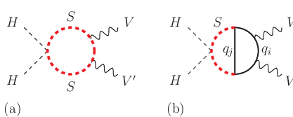In Fig.8 we show how we can generate these effective gauge-Higgs operators. One typical diagram to produce CP-even operator is Fig.8(a), which is at one-loop level. Based on a naive dimensional analysis, the Wilson coefficients are given [33]

		$\displaystyle\frac{c_{3}}{\Lambda^{2}}=\frac{3}{2}\frac{c_{2}}{\Lambda^{2}}=\frac{3}{2}\frac{c_{1}}{\Lambda^{2}}=\frac{2\lambda_{1}+\lambda_{2}}{64\pi^{2}m_{S}^{2}}\,,$
		$\displaystyle\frac{c_{12}}{\Lambda^{2}}=\frac{\lambda_{2}}{48\pi^{2}m_{S}^{2}}\,.$		(51)

And the CP violating operators are generated at two-loop level, see Fig.8(b). A ball park estimation gives

\frac{\tilde{c}_{1,2,12,3}}{\Lambda^{2}}\sim\sum_{i,j}\frac{\mathrm{Im}[u^{*}_{ij}v_{ij}]}{(16\pi^{2})^{2}}\frac{m_{q_{i}}m_{q_{j}}}{m_{S}^{2}\mathrm{max}\{m^{2}_{q_{i,j}},m_{H}^{2}\}}\,.

(52)

where $q_{i,j}$ are in the mass basis and the octet Yukawa are parameterized as $\bar{q}_{i}T^{A}(u_{ij}+v_{ij}\gamma^{5})q_{j}S^{A}$ . Even though the CP violating phase is of order one, the strength of $\tilde{c}$ ’s are roughly two orders smaller than the CP-even Wilson coefficients in this model.

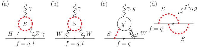Since this model is UV complete, we are able to discuss the fermion EDM and AMDM at above the electroweak scale without encountering any divergence. The charged lepton (g-2) starts at two-loop level, see Fig.9(a,b)⁴⁴ 4 The resulting 2-loop (g-2) can be read and translated from [51] where the similar diagrams due to exotic scalars have been considered. . Both Fig.9(a) and Fig.9(b) can be related to the diagram shown in Fig.8(a) by substituting VEV(s) for either one or two of external $H$ legs. And this is exactly what we have performed in the gauge-Higgs operator analysis for $\triangle a_{e}$ and $\triangle a_{\mu}$ .

For the most general Yukawa coupling, Eq.(50), the SM quarks receive nonzero EDM at 2-loop level, see Fig.9(c,d)⁵⁵ 5 The formulas in [52], where EDMs are generated via the similar diagrams in SUSY models, can be easily translated for use in this Octet model. . Both Fig.9(c) and Fig.9(d) are independent of Fig.8(b), and our gauge-Higgs operator estimations for quark EDMs are subleading. On the other hand, there are two kinds of contributions to the SM lepton EDM: (1) 3-loop diagrams, by connecting Fig.8(b) to the lepton line by either the SM Higgs or gauge bosons. These leading contributions have been taken care of by our gauge-Higgs operator analysis. (2) 4-loop diagrams, first by joining the two external quark lines to form a loop in Fig.9(c) or 9(d), and then connecting the resulting bulb to the lepton lines via either SM Higgs or gauge bosons. So our gauge-Higgs operator estimation for lepton EDM are indeed the leading contribution. Nevertheless, in the case that Yukawa couplings are most general, one needs to incorporate the Fermion EDM/ AMDM effective operators in the analysis, see [53] for an earlier study on the interplay of the 4-fermi operators and the electric and magnetic diploe operators.

To avoid the FCNC and other phenomenological problems, it is a common practice to assume that $Y_{ij}^{U/D}=\beta^{U/D}y_{ij}^{U/D}$ , where $\beta^{U/D}$ are real. In that case, both Yukawa are real in the fermion mass basis, and the contributions from Fig.9(c) and Fig.9(d) vanish. However, the CP violating gauge-Higgs operators, Fig.8(b), vanish as well and we do not have any say about the CP violation constraint. Assuming that $\Lambda=m_{S}=1\mathrm{TeV}$ , our numerical gives $-3\lesssim c_{1}\lesssim 4$ , $-2.5\lesssim c_{2}\lesssim 3$ , $-0.25\lesssim c_{12}\lesssim 0.25$ (from S parameter ), and $-0.02\lesssim c_{3}\lesssim 0.015$ , if we take the SM-like solution, then

	$\displaystyle-118\lesssim\lambda_{2}\lesssim 118\,,$
	$\displaystyle-12.6\lesssim 2\lambda_{1}+\lambda_{2}\lesssim 9.5\,.$		(53)

In addition to the positivity conditions for the scalar potential, Eq.(49), the above limits provide further nontrivial constrains on the parameter space of this model.

Based on the above discussion, one can tailor a modified UV complete model where our gauge-Higgs operator analysis is applicable. In one of the modified versions, the octet scalar is replaced by a real $SU(2)$ triplet, $S_{t}$ , which carries the SM quantum number $(8,3,0)$ . Because of the $SU(2)$ representation, it has no Yukawa couplings to all SM fermions and thus there is neither FCNC problems nor the EDM contributions from Fig.9(c) and Fig.9(d). The most general renormalizable potential of the Octet-triplet scalar is

$\displaystyle V(S_{t})$	$\displaystyle=$	$\displaystyle\frac{\lambda}{4}(H^{\dagger}H)^{2}+m_{S_{t}}^{2}\,\text{Tr}(S_{t}^{i}S_{t}^{i})+i\,\mu_{t}\,\epsilon^{ijk}\,\text{Tr}(S_{t}^{i}S_{t}^{j}S_{t}^{k})$	(54)
		$\displaystyle+\lambda_{t1}H^{\dagger}H\,\text{Tr}(S_{t}^{i}S_{t}^{i})+\lambda_{t2}\,\text{Tr}(S_{t}^{i}S_{t}^{i}S_{t}^{j}S_{t}^{j})+\lambda_{t3}\,\text{Tr}(S_{t}^{i}S_{t}^{j}S_{t}^{i}S_{t}^{j})$
		$\displaystyle+\lambda_{t4}\,\text{Tr}(S_{t}^{i}S_{t}^{i})\,\text{Tr}(S_{t}^{j}S_{t}^{j})+\lambda_{t5}\,\text{Tr}(S_{t}^{i}S_{t}^{j})\,\text{Tr}(S_{t}^{i}S_{t}^{j})$

where $i,j,k=1,2,3$ are the $SU(2)$ indices for adjoint representation. Moreover, we introduce a pair of exotic vector fermions, $\psi_{L,R}$ , whose SM quantum numbers are $(6,2,1/2)$ . The vector fermions admit a Dirac mass and a Yukawa coupling to $S_{t}$ ,

{\cal L}\supset m_{\psi}\bar{\psi}_{L}\psi_{R}+\eta_{t}\bar{\psi}_{L}S_{t}\psi_{R}+h.c.

(55)

The Dirac mass $m_{\psi}$ is taken to be real without losing any generality and assumed to be much larger than $v$ so that the exotic fermions decouple as $S_{t}$ does when energy is below the electroweak scale. The Yukawa $\eta_{t}$ is complex in general. The CP violating gauge-Higgs operators can be generated at two-loop levels, by replacing $(S,q)\rightarrow(S_{t},\psi)$ in Fig.8(b), and a rough estimation for the Wilson coefficients are

\frac{\tilde{c}_{1,2,12,3}}{\Lambda^{2}}\sim\frac{1}{(16\pi^{2})^{2}}\frac{\mathrm{Re}\,\eta_{t}\,\mathrm{Im}\,\eta_{t}}{\mathrm{max}\{m_{S_{t}}^{2},m_{\psi}^{2}\}}\,.

(56)

For $m_{S_{t}}\sim m_{\psi}\sim 1$ TeV, the $\theta_{QCD}$ gives the strongest constraint that $|\eta_{t}|^{2}|\sin 2\theta_{t}|<1.01\times 10^{-6}$ . The CP-even Wilson coefficients are generated at 1-loop level ( by replacing $S$ by $S_{t}$ in Fig.8(a) )

\frac{4}{3}\frac{c_{3}}{\Lambda^{2}}=\frac{3}{4}\frac{c_{2}}{\Lambda^{2}}=\frac{\lambda_{t1}}{16\pi^{2}m_{S_{t}}^{2}}\,,

(57)

but nonzero $c_{1}$ and $c_{12}$ need to be generated at higher-loop level since $S_{t}$ carries no hypercharge. And our global fit yields that $-4.2\leq\lambda_{t1}\leq 3.2$ .

6.3 Predictions for the CP-odd decays

The spin and parity of the 125 GeV boson has been largely determined to be $J^{P}=0^{+}$ from the analysis of the polar angular distribution in the $h\rightarrow 2\gamma$ mode[8, 16] (for spin) and the polarization correlation in the $h\rightarrow ZZ\rightarrow 4l$ decay[9, 17] (for parity). However, the current spin-parity analyses are all based on limited number of events and simple working assumptions, namely the boson is assumed to be either purely scalar, pseudoscalar, or spin-2 object ect. But we have to keep in mind that even the 125 GeV boson is an elementary scalar, the CP violation decays can still be generated by quantum corrections. For a given model, whether we have the required experimental sensitivity to detect the CP-odd composition is the question.

If at low energy the new physics can be indeed described by the gauge-Higgs operators alone, our numerical study predicts interesting model-independent relations among the Higgs CP-odd decay modes. As has been discussed in Sec.4, also from Fig.5(e,f), the three CP-odd Wilson coefficients follow a linear relation on a line segment with end points at $\tilde{c}^{2}_{12}\sim 0.56/1.0$ for using the SM predictions/ LHC data as input. For $\Lambda=1$ TeV, we have (c.f. Eq.(29))

$\displaystyle\alpha^{\not\!\!CP}_{\gamma\gamma}$	$\displaystyle\sim 3.21\,\tilde{c}^{2}_{12}\,,$	(58)
$\displaystyle\alpha^{\not\!\!CP}_{\gamma Z}$	$\displaystyle\sim 1.92\,\tilde{c}^{2}_{12}\,,$
$\displaystyle\alpha^{\not\!\!CP}_{ZZ}$	$\displaystyle\sim 4.3\times 10^{-5}\,\tilde{c}^{2}_{12}\,,$
$\displaystyle\alpha^{\not\!\!CP}_{WW}$	$\displaystyle\sim 1.13\times 10^{-4}\,\tilde{c}^{2}_{12}\,.$

Note that both $h\rightarrow WW$ and $h\rightarrow ZZ$ channels are not sensitive to the presence of the CP-odd gauge-Higgs operators.

We are interested in the CP violation fraction, $CPV_{ij}=\Gamma^{ij}_{\not\!\!CP}/\Gamma^{ij}$ , which is more relevant for the parity determination. In Fig.10, we show the $95\%$ CL CP violation fraction correlations between: (a) $h\to ZZ$ and $h\to\gamma\gamma$ , and (b) $h\to WW$ and $h\to\gamma\gamma$ . Note the possible large CPV fractions due to the gauge-Higgs effective operators in the $h\to\gamma\gamma$ and $h\to\gamma Z$ modes, which are not constrained at all by the global fit.

Apparently, it is not likely to probe the CP violation fractions, at the level of $\lesssim$ ( a few ) $\times 10^{-5}$ , in the $h\rightarrow WW,ZZ$ channels at the LHC⁶⁶ 6 See [54] for other proposals of measuring the CP nature of Higgs at the LHC.. This agrees with the current parity determination results[9, 17]. And hypothetically, any future observation of $\sim$ a few % level CP violation fraction in the $h\rightarrow ZZ$ mode will definitely indicate the existence of new physics beyond the gauge-Higgs sector and additional effective operators must be included.

For making use of $h\rightarrow 2\gamma,\gamma Z$ channels to probe the CP-odd components of the 125 GeV boson, we need to study the vector boson spin correlation. This could be neatly done in the future $e^{+}e^{-}$ , $e\gamma$ , or $\gamma\gamma$ colliders, see for example [55]. For that we have a model-independent prediction: $\alpha_{\not\!\!CP}^{\gamma\gamma}:\alpha_{\not\!\!CP}^{\gamma Z}\sim 1.67:1$ . However, as shown in Fig.11, when the above relation is converted into the CPV fraction, the relation is smeared but more or less follows a linear relation. From the plot, the CPV fraction correlation between these two modes is roughly

CPV_{\gamma z}\sim(0.65\pm 0.35)CPV_{\gamma\gamma}\;\;(68\%\mbox{CL}).

(59)

However, the slope becomes $(0.92\pm 0.7)$ for the $95\%$ CL fit. Although not being very predictive, this prediction can be checked once the experimental sensitivities meet the SM theoretical uncertainties and the CPV fractions in $\gamma\gamma$ and $\gamma Z$ modes are measured in the future.

Nevertheless, from our numerical study, we found potentially large CP violating compositions in the $h\to\gamma\gamma,\gamma Z$ decays.

6.4 Summary

We have studied the new physics associated with the 125 GeV boson where the NP is assumed to be characterized by the effective gauge-Higgs operators. By global fitting we studied the correlations among various Higgs to di-boson decay modes. In addition to the updated Higgs measurements accumulated at the LHC, we also considered the case when the experimental sensitivities are compatible with the SM theoretic uncertainties. We found that there is plenty of room for new physics to hide in the shadow of the inherent SM theoretical uncertainties. From the global fit, we found a robust prediction that $\mu_{ZZ}\simeq\mu_{WW}$ and $0.6\lesssim\mu_{ZZ,WW}\lesssim 1.4$ at $95\%$ CL, see Figs.4 and 7. This can be tested at the LHC with more data in the near future.

Moreover, we take into account the constraints of EDMs and AMDMs under the assumption that the gauge-Higgs operators give the dominate contributions to them. We found very strong constraints on the CP-odd Wilson coefficients and our numerical indicated that the CP violating $hVV$ interactions in the $h\rightarrow WW$ and $h\rightarrow ZZ$ modes are too small, $\sim{\cal O}(10^{-5})$ at most, to be detected at the LHC, see Fig.10. However, the CP-odd fraction in the $h\gamma\gamma$ and $h\gamma Z$ channels could be as large as ${\cal O}(1)$ .

Two more intriguing relations are predicted if the EDM constraints are included: (1) $(\alpha_{WW}-1)\sim 2(\alpha_{ZZ}-1)$ , and (2) $(\alpha_{\gamma Z}-1)\sim 6500(\alpha_{WW}-1)^{2}$ . These predictions could be tested at the future precision Higgs machines.

The caveats: we should keep in mind that our results are valid only for the class of NP which manifests itself in the form of the gauge-Higgs operators discussed in this work. So our results are not applicable if (1) existence of any light exotic degree of freedom below the electroweak scale which interacts with the Higgs boson, or (2) the NP is beyond the realm which can be largely charted by the gauge-Higgs operators. On the other hand, any violation of our above predictions will indicate that the new physics must go beyond the gauge-Higgs sector.

Acknowledgments.

Work was supported by the Taiwan NSC, Grant No. 99-2112-M-007-006-MY3. FX is also supported by the Taiwan NSC, Grant No. 101-2811-M-007-051 .

Appendix A Decay width of $h\rightarrow WW^{},ZZ^{}$

Details of calculating the width of $h\rightarrow VV^{*}$ ( $V=W,Z$ ) are collected in this section. We consider the case that the virtute gauge boson $V^{*}$ subsequently decays into two fermions $f$ and $f^{\prime}$ with their momentums labeled as: $h(P)\rightarrow V(p_{1})+f(p_{2})+f^{\prime}(p_{3})$ . In the center of mass frame of $f$ and $f^{\prime}$ , the three-body decay width is given by the following phase integral

		$\displaystyle\Gamma=\frac{1}{256\pi^{3}m_{h}^{3}}\int^{(M-m_{1})^{2}}_{(m_{2}+m_{3})^{2}}ds_{1}\int^{s_{2+}}_{s_{2-}}ds_{2}\left(\|\mathcal{M}_{1}\|^{2}+\|\mathcal{M}_{2}\|^{2}\right)\,,$		(60)
		$\displaystyle s_{2\pm}=m_{1}^{2}+m_{3}^{2}+\frac{1}{2s_{1}}\left[(s-s_{1}-m_{1}^{2})(s_{1}+m_{3}^{2}-m_{2}^{2})\pm\lambda^{\frac{1}{2}}(s_{1},m_{3}^{2},m_{2}^{2})\lambda^{\frac{1}{2}}(s_{1},M^{2},m_{1}^{2})\right]\,,$
		$\displaystyle\lambda(a,b,c)\equiv a^{2}+b^{2}+c^{2}-2ab-2ac-2bc\,,$		(61)

where the kinematical variables are defined as: $s=P^{2}$ , $p_{4}\equiv(p_{2}+p_{3})$ , $s_{1}=p_{4}^{2}$ , $s_{2}=(p_{1}+p_{3})^{2}$ , $s_{3}=(p_{1}+p_{2})^{2}$ , and $\mathcal{M}_{1}$ and $\mathcal{M}_{2}$ are the CP-even and CP-odd amplitudes respectively The phase space integral is largely simplified when the final state fermions are massless which is a good approximation in our case.

Beside the SM contribution, the CP-even amplitude also receives the contributions from ${\cal O}_{1}$ and ${\cal O}_{2}$ and

	$\displaystyle\|\mathcal{M}_{1}\|^{2}$	$\displaystyle=$	$\displaystyle\frac{4N_{c}^{f}(g_{V}^{2}+g_{A}^{2})}{(s_{1}-m_{V}^{2})^{2}}\times\left[\left(m_{V}^{2}4\sqrt{2}G_{F}-a_{V}^{{}^{\prime}2}s_{1}\right)(2p_{1}\cdot p_{2}p_{1}\cdot p_{3}-p_{1}^{2}p_{2}\cdot p_{3})\right.$		(62)
			$\displaystyle\left.\hskip 93.89418pt+(m_{V}^{2}2(\sqrt{2}G_{F})^{\frac{1}{2}}-a_{V}^{{}^{\prime}}p_{1}\cdot p_{4})^{2}2p_{2}\cdot p_{3}\right]\,,$		(62)

where $a^{\prime}_{W}=2c_{2}vg_{2}^{2}/\Lambda^{2}$ , $a^{\prime}_{Z}=2a_{4}vg_{2}^{2}/\Lambda^{2}$ , $N_{c}^{f}$ the color factor of the final state fermions, and $(g_{V},g_{A})=(g_{2}/2c_{W})(I_{3}-2Q_{f}s_{W}^{2},-I_{3})$ for $Z^{0}$ and $g_{V}=-g_{A}=g_{2}/2\sqrt{2}$ for $W^{\pm}$ . And $\mathcal{M}_{2}$ is completely beyond the SM,

	$\displaystyle\|\mathcal{M}_{2}\|^{2}=8(g_{V}^{2}+g_{A}^{2})\left(\frac{\tilde{a}^{\prime}_{V}}{s_{1}-m_{V}^{2}}\right)^{2}\times\left[(p_{1}\cdot p_{4})(p_{3}\cdot p_{4}p_{1}\cdot p_{2}+p_{2}\cdot p_{4}p_{1}\cdot p_{3})\right.$
	$\displaystyle\left.-p_{4}^{2}p_{1}\cdot p_{2}p_{1}\cdot p_{3}-p_{1}^{2}p_{2}\cdot p_{4}p_{3}\cdot p_{4}\right]\,,$		(63)

where $\tilde{a}^{\prime}_{W}=2\tilde{c}_{2}vg_{2}^{2}/\Lambda^{2}$ , and $\tilde{a}^{\prime}_{Z}=2\tilde{a}_{4}vg_{2}^{2}/\Lambda^{2}$ . Summing up all massless final states, the corresponding CP-even decay widths are:

		$\displaystyle\Gamma_{1}^{W}=\frac{9G_{F}^{2}m_{W}^{4}m_{h}}{8\pi^{3}}R_{1}(m_{W}/m_{h},a_{W}^{\prime})\qquad(\mathrm{for}~W)\,,$
		$\displaystyle\Gamma_{1}^{Z}=\frac{3G_{F}^{2}m_{Z}^{4}m_{h}}{32\pi^{3}}\delta_{Z}R_{1}(m_{Z}/m_{h},a_{Z}^{\prime})\qquad(\mathrm{for}~Z)\,,$		(64)

with $\delta_{Z}=\left(7-\frac{40}{3}s_{W}^{2}+\frac{160}{9}s_{W}^{4}\right)$ , the phase space factor $R_{1}$ will be given in below. The $\delta_{Z}$ factor is different from [36] and differs by a factor of 3 for W case, but our results are consistent with [56].

For the CP-odd part, the decay widths for W and Z bosons are

		$\displaystyle\Gamma_{2}^{W}=\tilde{c}_{2}^{2}\frac{9m_{h}^{3}g_{2}^{6}v^{2}}{32\pi^{3}\Lambda^{4}}R_{2}(\epsilon)=\tilde{c}^{2}_{2}\frac{9G_{F}^{2}m_{W}^{4}m_{h}}{8\pi^{3}}\cdot\frac{32m_{h}^{2}m_{W}^{2}}{\Lambda^{4}}R_{2}(\epsilon)\,,$
		$\displaystyle\Gamma_{2}^{Z}=\tilde{a}^{2}_{4}\delta_{Z}\frac{3G_{F}^{2}m_{Z}^{4}m_{h}}{32\pi^{3}}\cdot\frac{32m_{h}^{2}m_{Z}^{2}c_{W}^{4}}{\Lambda^{4}}R_{2}(\epsilon)\,.$		(65)

The two functions $R_{1},R_{2}$ can be expressed in the form of integrals,

		$\displaystyle R_{1}(\epsilon,a_{V}^{\prime})\equiv\epsilon^{2}\int^{(1-\epsilon)^{2}}_{0}d\tilde{s}_{1}\int^{\tilde{s}_{2+}}_{\tilde{s}_{2-}}d\tilde{s}_{2}\frac{1}{(\tilde{s}_{1}-\epsilon^{2})^{2}}$
		$\displaystyle\hskip 28.45274pt\left\{\left(1-\frac{a_{V}^{{}^{\prime}2}\tilde{s}_{1}}{4\sqrt{2}G_{F}\epsilon^{2}}\right)\left((1-\tilde{s}_{1}-\tilde{s}_{2})(\tilde{s}_{2}-\epsilon^{2})\frac{1}{\epsilon^{2}}-\tilde{s}_{1}\right)+2\tilde{s}_{1}\left(1-a^{\prime}_{V}\frac{1-\epsilon^{2}-\tilde{s}_{1}}{4(\sqrt{2}G_{F})^{\frac{1}{2}}\epsilon^{2}}\right)^{2}\right\}\,,$
		$\displaystyle R_{2}(\epsilon)\equiv\int^{(1-\epsilon)^{2}}_{0}d\tilde{s}_{1}\int^{\tilde{s}_{2+}}_{\tilde{s}_{2-}}d\tilde{s}_{2}\frac{\tilde{s}_{1}}{(\tilde{s}_{1}-\epsilon^{2})^{2}}\left[\frac{1}{4}(1-\epsilon^{2}-\tilde{s}_{1})^{2}-\frac{1}{2}\epsilon^{2}\tilde{s}_{1}-\frac{1}{2}(\tilde{s}_{2}-\epsilon^{2})(1-\tilde{s}_{1}-\tilde{s}_{2})\right]\,,$

with the relevant parameters introduced as $\epsilon=\frac{m_{V}}{m_{h}}$ , $\tilde{s}_{1}=\frac{s_{1}}{m_{h}^{2}}$ , $\tilde{s}_{2}=\frac{s_{2}}{m_{h}^{2}}$ , and $\tilde{s}_{2\pm}=\frac{1}{2}(1+\epsilon^{2}-\tilde{s}_{1})\pm\frac{1}{2}\sqrt{[(1+\epsilon)^{2}-\tilde{s}_{1}][(1-\epsilon)^{2}-\tilde{s}_{1}]}$ . The analytical form for $R_{1,2}$ can be obtained:

		$\displaystyle R_{1}(\epsilon,a)=-\frac{1}{72\epsilon^{2}}\left[A+B\arctan\frac{(1-\epsilon^{2})\sqrt{4\epsilon^{2}-1}}{1-3\epsilon^{2}}+C\ln\epsilon\right]\,,$		(66)
		$\displaystyle\hskip 28.45274ptA=(1-\epsilon^{2})\left[36a\epsilon^{2}(-5+9\epsilon^{2})+6(2-13\epsilon^{2}+47\epsilon^{4})+a^{2}(17-82\epsilon^{2}+89\epsilon^{4})\right]\,,$
		$\displaystyle\hskip 28.45274ptB=\frac{6}{\sqrt{4\epsilon^{2}-1}}\left[6(\epsilon^{2}-8\epsilon^{4}+20\epsilon^{6})+12a(\epsilon^{2}-8\epsilon^{4}+14\epsilon^{6})+a^{2}(-1+11\epsilon^{2}-40\epsilon^{4}+54\epsilon^{6})\right]\,,$
		$\displaystyle\hskip 28.45274ptC=6\left[6(\epsilon^{2}-6\epsilon^{4}+4\epsilon^{6})+12a(\epsilon^{2}-6\epsilon^{4}+2\epsilon^{6})+a^{2}(-1+9\epsilon^{2}-30\epsilon^{4}+6\epsilon^{6})\right]\,,$
		$\displaystyle R_{2}(\epsilon)=\frac{(1-\epsilon^{2})}{36}\left(-17+64\epsilon^{2}+\epsilon^{4}\right)+\frac{\ln\epsilon}{6}(1+6\epsilon^{4}-9\epsilon^{2})$
		$\displaystyle\hskip 42.67912pt+\frac{(7\epsilon^{2}-1)}{6}\sqrt{4\epsilon^{2}-1}\arctan\frac{(\epsilon^{2}-1)\sqrt{4\epsilon^{2}-1}}{3\epsilon^{2}-1}\,,$		(67)

References

- [1] ATLAS Collaboration, Phys. Lett. B 716 (2012) 1-29; 1207.7214 [hep-ex].
- [2] CMS Collaboration, Phys. Lett. B 716 (2012) 30-61; 1207.7235 [hep-ex];
- [3] Fabrice Hubaut, ”Latest ATLAS studies on Higgs to diboson states”, talk given in Moriond-2013, EW.
- [4] E. Mountricha, ”Study of Higgs production in Bosonic Decay Channels at ATLAS”, talk given in Moriond-2013, QCD.
- [5] Victoria Martin,, ”Searches for the BEH boson into fermions at ATLAS”, talk given in Moriond-2013, EW.
- [6] D. Puigh, ”Searches for Standard Model Scalar Boson Decaying to Fermions at the LHC”, talk given in Moriond-2013, QCD.
- [7] ATLAS collaboration, ATLAS-CONF-2013-009.
- [8] ATLAS collaboration, ATLAS-CONF-2013-012.
- [9] ATLAS collaboration, ATLAS-CONF-2013-013.
- [10] ATLAS collaboration, ATLAS-CONF-2013-030.
- [11] ATLAS collaboration, ATLAS-CONF-2012-160.
- [12] ATLAS collaboration, ATLAS-CONF-2012-161.
- [13] Guillelmo Gómez-Ceballos, ”Study of Standard Model Scalar Production in Bosonic Decay Channels in CMS”, talk given in Moriond-2013, EW.
- [14] C. Ochando, ”Study of Higgs production in Bosonic Decays Channels in CMS”, talk given in Moriond-2013, QCD.
- [15] Valentina Dutta, ”Search for the Standard Model Scalar Boson Decaying to Fermions at CMS”, talk given in Moriond-2013, EW.
- [16] CMS collaboration, CMS PAS HIG-13-001.
- [17] CMS collaboration, CMS PAS HIG-13-002.
- [18] CMS collaboration, CMS PAS HIG-13-003.
- [19] CMS collaboration, CMS PAS HIG-13-004.
- [20] CMS collaboration, CMS PAS HIG-13-006.
- [21] J. Cao, Z. Heng, T. Liu and J. M. Yang, Phys. Lett. B 703, 462 (2011); C. Englert, T. Plehn, D. Zerwas and P. M. Zerwas, Phys. Lett. B 703, 298 (2011);Y. Bai, J. Fan and J. L. Hewett, JHEP 1208, 014 (2012);M. Carena, S. Gori, N. R. Shah and C. E. M. Wagner, JHEP 1203, 014 (2012);U. Ellwanger, JHEP 1203 (2012) 044;A. Arvanitaki and G. Villadoro, JHEP 1202, 144 (2012);B. Batell, S. Gori and L. -T. Wang, JHEP 1206, 172 (2012);A. Arhrib, R. Benbrik, M. Chabab, G. Moultaka and L. Rahili, JHEP 1204, 136 (2012); A. Arhrib, R. Benbrik and N. Gaur, Phys. Rev. D85, 095021 (2012);S. Kanemura and K. Yagyu, Phys. Rev. D 85 (2012) 115009;D. Carmi, A. Falkowski, E. Kuflik and T. Volansky, JHEP 1207, 136 (2012);A. Azatov, R. Contino and J. Galloway, JHEP 1204, 127 (2012);J. R. Espinosa, C. Grojean, M. Muhlleitner and M. Trott, JHEP 1205, 097 (2012);P. Draper and D. McKeen, Phys. Rev. D 85, 115023 (2012);Dawson and Furlan, Phys.Rev. D86 (2012)01502; Carena, Gori, Shah, Wagner, and Wang, JHEP 1207 (2012)175; Akeroyd and Moretti, Phys.Rev. D86 (2012)035015; Carena, Low, and Wagner, JHEP 1208 (2012) 060; J. A. Azatov, R. Contino, D. Del Re, J. Galloway, M. Grassi and S. Rahatlou, JHEP 1206 (2012) 134;M. Klute, R. Lafaye, T. Plehn, M. Rauch and D. Zerwas, Phys. Rev. Lett. 109, 101801 (2012);K. Kumar, R. Vega-Morales and F. Yu, Phys. Rev. D 86, 113002 (2012);L. Wang and X. -F. Han, Phys. Rev. D 86, 095007 (2012);N. Bonne and G. Moreau, Phys. Lett. B 717, 409 (2012);J. Cao, Z. Heng, J. M. Yang and J. Zhu, JHEP 1210, 079 (2012);W. -F. Chang, J. N. Ng and J. M. S. Wu, Phys. Rev. D86(2012)033003;T. Corbett, O. J. P. Eboli, J. Gonzalez-Fraile and M. C. Gonzalez-Garcia, Phys. Rev. D86 (2012) 075013;J. Baglio, A. Djouadi and R. M. Godbole, Phys. Lett. B716, 203 (2012);M. Montull and F. Riva, JHEP 1211 (2012) 018;J. R. Espinosa, C. Grojean, M. Muhlleitner and M. Trott, JHEP 1212, 045 (2012);S. Banerjee, S. Mukhopadhyay and B. Mukhopadhyaya, JHEP 1210 (2012) 062;A. Joglekar, P. Schwaller and C. E. M. Wagner, JHEP 1212, 064 (2012);F. Bonnet, T. Ota, M. Rauch and W. Winter, Phys. Rev. D 86 (2012) 093014;J. R. Espinosa, C. Grojean, V. Sanz and M. Trott, JHEP 1212, 077 (2012);Bellazzini, Petersson, and Torre, Phys.Rev. D86 033016(2012); Ke, Luo, Shan, Wang, and Wang, Phys.Lett. B7181334 (2013); Low, Lykken, and Shaughnessy, Phys.Rev. D86 093012(2012); Giardino, Kannike, Raidal, and Strumia, Phys.Lett. B718 469(2012); Buckley and Hooper, Phys.Rev. D86 075008(2012); Carmi, Falkowski, Kuflik, Volansky, and Zupan, JHEP 1210 196 (2012); An, Liu, and Wang, Phys.Rev. D86 075030(2012); Abe, Chen, and He, JHEP 1301 082(2013); Bertolini and McCullough, JHEP 1212 118(2012); Joglekar, Schwaller, and Wagner, JHEP 1212 064(2012); N. Arkani-Hamed, K. Blum, R. T. D’Agnolo and J. Fan, JHEP 1301, 149 (2013);N. Haba, K. Kaneta, Y. Mimura and R. Takahashi, Phys. Lett. B718 (2013) 1441;Almeida, Bertuzzo, Machado, and Funchal, JHEP 1211 (2012) 085; D. S. M. Alves, P. J. Fox and N. J. Weiner, arXiv:1207.5499 [hep-ph]; Batell, McKeen, and Pospelov, JHEP 1210 (2012) 104; Giudice, Paradisi, and Strumia, JHEP1210 (2012) 186; Delgado, Nardini, and Quiros, Phys.Rev. D86 (2012) 115010; Kearney, Pierce, and Weiner, Phys.Rev. D86 (2012) 113005; M. Hashimoto and V. A. Miransky, Phys. Rev. D86, 095018 (2012);Schmidt-Hoberg and Staub, JHEP 1210 (2012) 195; M. Reece, arXiv:1208.1765 [hep-ph]; Davoudiasl, Lee, and Marciano, Phys.Rev. D86 (2012) 095009; Cai, Chao, and Yang, JHEP 1212 (2012) 043; Bae, Jung, and Kim, Phys.Rev. D87(2013) 015014; Voloshin, Phys.Rev. D86 (2012) 093016; Kitahara, JHEP 1211 (2012) 021; Chun, Lee, and Sharma, JHEP 1211 (2012) 106; Lee, Park, and Park, JHEP 1212 (2012) 037; E. Bertuzzo, P. A. N. Machado and R. Zukanovich Funchal, JHEP 1302, 086 (2013); B. Batell, S. Gori and L. -T. Wang, JHEP 1301, 139 (2013); W. Huang, J. Shu and Y. Zhang, JHEP 1303, 164 (2013); Altmannshofer, Gori, and Kribs, Phys.Rev. D86 (2012) 115009; G. Moreau, Phys. Rev. D87, 015027 (2013);C. -Q. Geng, D. Huang, Y. Tang and Y. -L. Wu, Phys. Lett. B719, 164 (2013);Chala, JHEP 1301 (2013) 122; I. Picek and B. Radovcic, Phys. Lett. B719, 404 (2013);K. Choi, S. H. Im, K. S. Jeong and M. Yamaguchi, JHEP 1302, 090 (2013);B. Batell, S. Jung and H. M. Lee, JHEP 1301, 135 (2013);Schmidt-Hoberg, Staub, and Winkler, JHEP 1301 (2013) 124; H. Davoudiasl, I. Lewis and E. Ponton, arXiv:1211.3449 [hep-ph]; T. Corbett, O. J. P. Eboli, J. Gonzalez-Fraile and M. C. Gonzalez-Garcia, Phys. Rev. D87, 015022 (2013);M. Carena, S. Gori, I. Low, N. R. Shah and C. E. M. Wagner, JHEP 1302, 114 (2013);F. Arbabifar, S. Bahrami and M. Frank, Phys. Rev. D87, 015020 (2013);M. Berg, I. Buchberger, D. M. Ghilencea and C. Petersson, arXiv:1212.5009 [hep-ph]; G.-n. Li, G. Guo, B. Ren, Y.-J. Zheng, X.-G. He, 1212.5528[hep-ph]; C. Han, N. Liu, L. Wu, J. M. Yang and Y. Zhang, arXiv:1212.6728 [hep-ph]; W. Chao, J. -H. Zhang and Y. Zhang, arXiv:1212.6272 [hep-ph]; S. Funatsu, H. Hatanaka, Y. Hosotani, Y. Orikasa and T. Shimotani, arXiv:1301.1744 [hep-ph]; J. Fan and M. Reece, arXiv:1301.2597 [hep-ph]; P.S. Bhupal Dev, D.K. Ghosh, N. Okada and I. Saha, 1301.3453[hep-ph]; Phys. Rev. D 87 (2013) 015022; J. Cao, L. Wu, P. Wu and J. M. Yang, arXiv:1301.4641 [hep-ph]; C. -S. Chen, C. -Q. Geng, D. Huang and L. -H. Tsai, arXiv:1301.4694 [hep-ph]; C. Cheung, S. D. McDermott and K. M. Zurek, arXiv:1302.0314; W. -Z. Feng and P. Nath, arXiv:1303.0289 [hep-ph]; A. Falkowski, F. Riva and A. Urbano, arXiv:1303.1812;
- [22] https://twiki.cern.ch/twiki/bin/view/LHCPhysics/CrossSections
- [23] https://twiki.cern.ch/twiki/bin/view/AtlasPublic/ExoticsPublicResults
- [24] https://twiki.cern.ch/twiki/bin/view/CMSPublic/PhysicsResultsEXO .
- [25] W. Buchmüller and D. Wyler, Nucl. Phys. B 268 (1986), 621-653.
- [26] B. Grzadkowski, M. Iskrzynski, M. Misiak, J. Rosiek, JHEP 10 (2010) 085.
- [27] X. Zhang and B.-L. Young, Phys. Rev. D 49, 563 (1994).
- [28] D. McKeen, M. Pospelov and A. Ritz, Phy. Rev. D 86, 113004 (2012); 1208.4597 [hep-ph].
- [29] A.V. Manohar, M.B. Wise, Phys. Lett. B 636 (2006) 107-113; hep-ph/0601212.
- [30] Christophe Grojean, Elizabeth E. Jenkins, Aneesh V. Manohar, Michael Trotta, arXiv: 1301.2588 [hep-ph]; J. E.-Miró, J.R. Espinosaa, E. Massoa, A. Pomarol, arXiv: 1302. 5661v1 [hep-ph].
- [31] E. Masso and V. Sanz, arXiv: 1211. 1320[hep-ph]; P. Agrawal, S. Mitra, A. Shivaji, 1211. 4362 [hep-ph]; C. Degrande, N. Greiner, W. Kilian, O. Mattelaer, H. Mebane, T. Stelzer, S. Willenbrock, C. Zhang, 1205.4231 [hep-ph]; F. Bonnet, M. B. Gavela, T. Ota, W. Winter, Phys.Rev. D 85 (2012) 035016; S. Banerjee, S. Mukhopadhyay and B. Mukhopadhyaya, JHEP 10 (2012) 062; G. Belanger, B. Dumont, U. Ellwanger, J.F. Gunion, S. Kraml, JHEP 1302 (2013) 053; T. Corbett, O.J.P. Eboli, J. Gonzalez-Fraile, M.C. Gonzalez-Garcia, Phys.Rev. D87 (2013) 015022; B. Batell, S. Gori, L.-T. Wang, JHEP 1206 (2012) 172; R. Alonso, M. B. Gavela, L. Merlo, S. Rigolin, and J. Yepes, arXiv:1212.3305 [hep-ph]; R. Alonso, M. B. Gavela, L. Merlo, S. Rigolin, and J. Yepes, arXiv:1212.3307 [hep-ph].
- [32] A. Azatov, J. Galloway and , Int. J. Mod. Phys. A 28, 1330004 (2013); R. Contino, M. Ghezzi, C. Grojean, M. Mühlleitner and M. Spira, arXiv: 1303.3876v1 [hep-ph]; J. Ellis and T. You, arXiv: 1303.3879v1 [hep-ph]; A. Falkowski, F. Riva, A. Urbano, arXiv: 1303.1812v2 [hep-ph]; A. Djouadi and G. Moreau, arXiv: 1303.6591v1 [hep-ph].
- [33] A.V. Manohar and M.B. Wise, Phys. Rev. D 74, 035009 (2006).
- [34] M.E. Peskin and T. Takeuchi, Phys. Rev. D 46, 381 (1992); Phys. Rev. Lett. 8, 964 (1990).
- [35] J. Erler and P. Langacker “Electroweak model and constraints on new physics”, PDGLive.
- [36] A. Djouadi, Phys. Rept. 457 (2008) 1-216.
- [37]
B.L. Ioffe and V.A. Khoze, Sov. J. Part. Nucl. 9 (1978) 50 [Fiz. Elem. Chast. Atom.
Yadra 9 (1978) 118]; M.A.Shifman, A.I.Vainshtein, M.B. Voloshin, and V.I. Zakharov,
Sov. J. Nucl. Phys. 30 (1979) 711 [Yad. Fiz. 30 (1979) 1368].
R. Gastmans, S.L. Wu, T.T. Wu, 1108.5872 [hep-ph]; D. Huang, Y. Tang, Y.-L. Wu, 1109.4846v2 [hep-ph]. - [38] J.F. Gunion, H.E. Haber, G. Kane, S. Dawson, “The Higgs Hunter’s Guide”, Westview Press, 2000.
- [39] L.Bergstrom and G. Hulth, Nucl. Phys. B 259 (1985) 137 [Erratum-ibid. B 276 (1986) 744].
- [40] M. Pospelov and A. Ritz, hep-ph/0010037v2.
- [41] F. Xu, H. An, and X. Ji, JHEP 1003, 088 (2010).
- [42] W. Dekens, and J. de Vries, arXiv:1303.3156 [hep-ph].
- [43] J.J. Hudson, D.M. Kara, I.J. Smallman, B.E. Sauer, M.R. Tarbutt and E.A. Hinds, Nature 473, 493 (2011).
- [44] C.A. Baker, et. al. Phys. Rev. Lett. 97, 131801 (2006).
- [45] I. Bars and M. Yoshimura, Phys. Rev. D 6 (1972) 374; K. Fujikawa, B.W. Lee and A.I. Sanda, Phys. Rev. D 6(1972) 2923; W.A. Bardeen, R. Gastmans and B. Lautrup, Nucl. Phys. B 46 (1972), 319-331.
- [46] G.W. Bennett, et. at. (Muon (g-2) Collaboration)), Phys. Rev. D 73, 072003 (2006).
- [47] G.F. Giudice, P. Paradisi, M. Passera, JHEP 1211 (2012) 113; 1208.6583 [hep-ph].
- [48] V. Barger, M. Ishida and W.-Y. Keung, Phys. Rev. Lett. 108, 261801 (2012).
- [49] T. Phehn, M. Spira, P.M. Zerwas, Nucl. Phys. B 479 (1996) 46-64.
- [50] X.-G. He, G. Valencia, H. Yokoya, JHEP 1112 (2011) 030; C. P. Burgess, M. Trott and S. Zuberi, JHEP 0909, 082 (2009); L. M. Carpenter and S. Mantry, arXiv:1104.5528 [hep-ph]. J. Cao, P. Wan, J. M. Yang and J. Zhu, arXiv:1303.2426 [hep-ph].
- [51] See for example, K. -m. Cheung, C. -H. Chou and O. C. W. Kong, Phys. Rev. D 64, 111301 (2001); D. Chang, W. -F. Chang, C. -H. Chou and W. -Y. Keung, Phys. Rev. D 63, 091301 (2001).
- [52] See for example, T. H. West, Phys. Rev. D 50, 7025 (1994); T. Kadoyoshi and N. Oshimo, Phys. Rev. D 55, 1481 (1997); D. Chang, W. -Y. Keung and A. Pilaftsis, Phys. Rev. Lett. 82, 900 (1999) [Erratum-ibid. 83, 3972 (1999)]; A. Pilaftsis, Phys. Lett. B 471, 174 (1999); D. Chang, W. -F. Chang and W. -Y. Keung, Phys. Lett. B 478, 239 (2000); D. Chang, W. -F. Chang and W. -Y. Keung, Phys. Rev. D 71, 076006 (2005); G. F. Giudice and A. Romanino, Phys. Lett. B 634, 307 (2006).
- [53] W. -F. Chang and J. N. Ng, JHEP 0510, 091 (2005); W. -F. Chang and J. N. Ng, hep-ph/0512334.
- [54] T. Plehn, D. L. Rainwater and D. Zeppenfeld, Phys. Rev. Lett. 88, 051801 (2002); V. Hankele, G. Klamke, D. Zeppenfeld and T. Figy, Phys. Rev. D 74, 095001 (2006); G. Klamke and D. Zeppenfeld, JHEP 0704, 052 (2007); F. Campanario, M. Kubocz and D. Zeppenfeld, Phys. Rev. D 84, 095025 (2011); C. Englert, M. Spannowsky and M. Takeuchi, JHEP 1206, 108 (2012); S. Berge and W. Bernreuther, Phys. Lett. B 671, 470 (2009); S. Berge, W. Bernreuther, B. Niepelt and H. Spiesberger, Phys. Rev. D 84, 116003 (2011); B. Coleppa, K. Kumar and H. E. Logan, Phys. Rev. D 86, 075022 (2012).
- [55] K. Hagiwara, and M. L. Stong, Z. Phys. C 62, 99 (1994); M. Kramer, J. H. Kuhn, M. L. Stong, P. M. Zerwas and , Z. Phys. C 64, 21 (1994); G. J. Gounaris, F. M. Renard, N. D. Vlachos and , Nucl.Phys. B 459, 51 (1996); S. Y. Choi, K. Hagiwara, M. S. Baek and , Phys. Rev. D 54, 6703 (1996); G. J. Gounaris, G. P. Tsirigoti and , Phys. Rev. D 56, 3030 (1997) [Erratum-ibid. D 58, 059901 (1998)]; E. Gabrielli, V. A. Ilyin, B. Mele and , Phys. Rev. D 60, 113005 (1999); I. F. Ginzburg, Nucl. Phys. Proc. Suppl. 82, 367 (2000); I. F. Ginzburg, I. P. Ivanov and , Eur. Phys. J. C 22, 411 (2001).
- [56] W.-Y. Keung and W.J. Marciano, Phys. Rev. D(R), 30 (1984)248.