跳到论文正文
W Papers独立论文阅读器 arXiv:1303.6923 论文正文 计算阅读时间 · 0%
引用这篇论文根据当前论文元数据生成,正式投稿前建议核对。


License: arXiv.org perpetual non-exclusive license
arXiv:1303.6923v3 [math.NA] 30 Oct 2013

Coupled BEM-FEM for the convected Helmholtz equation with non-uniform flow in a bounded domain

Fabien Casenave Affiliation: Université Paris-Est, CERMICS (ENPC), 6-8 Avenue Blaise Pascal, Cité DescartesF-77455 Marne-la-Vallée, France Affiliation: EADS-IW, 18 rue Marius Terce, 31300 Toulouse, France    Alexandre Ern Affiliation: Université Paris-Est, CERMICS (ENPC), 6-8 Avenue Blaise Pascal, Cité DescartesF-77455 Marne-la-Vallée, France    Guillaume Sylvand Affiliation: EADS-IW, 18 rue Marius Terce, 31300 Toulouse, France
Abstract

We consider the convected Helmholtz equation modeling linear acoustic propagation at a fixed frequency in a subsonic flow around a scattering object. The flow is supposed to be uniform in the exterior domain far from the object, and potential in the interior domain close to the object. Our key idea is the reformulation of the original problem using the Prandtl–Glauert transformation on the whole flow domain, yielding (i) the classical Helmholtz equation in the exterior domain and (ii) an anisotropic diffusive PDE with skew-symmetric first-order perturbation in the interior domain such that its transmission condition at the coupling boundary naturally fits the Neumann condition from the classical Helmholtz equation. Then, efficient off-the-shelf tools can be used to perform the BEM-FEM coupling, leading to two novel variational formulations for the convected Helmholtz equation. The first formulation involves one surface unknown and can be affected by resonant frequencies, while the second formulation avoids resonant frequencies and involves two surface unknowns. Numerical simulations are presented to compare the two formulations.

1 Introduction

The scope of the present work is the computation of linear acoustic wave propagation at a fixed frequency in the presence of a flow. When the flow is at rest, the simplest model is the classical Helmholtz equation for the acoustic potential. This equation can be reduced to finding unknown functions defined on the surface of the scattering object and solving integral equations which can be effectively approximated by the Boundary Element Method (BEM) [41]. When the medium of propagation is non-uniform, a volumic resolution has to be considered using, e.g., a Finite Element Method (FEM). If such non-uniformities occur only in a given bounded domain, it is possible to benefit from the advantages of both a volumic resolution and an integral equation formulation. Coupling BEM and FEM at the boundary of the given bounded domain allows this. Coupled BEM-FEM can be traced back to McDonald and Wexler [34], Zienkiewicz, Kelly and Bettess [45], Johnson and Nédélec [26] and Jin and Liepa [25]. Over the last decade, such methods have been investigated, among others, for electromagnetic scattering [21, 29, 30], elasticity [11], and fluid-structure [13] or solid-solid interactions [33, 44]. Coupled BEM-FEM for the classical Helmholtz equation can present resonant frequencies, leading to infinitely many solutions. All these solutions deliver the same acoustic potential in the exterior domain, but the numerical procedure becomes ill-conditioned. This problem has been solved in [8, 22], where a stabilization of the coupling, based on combined field integral equations (CFIE), has been proposed by introducing an additional unknown at the coupling surface.

When the medium of propagation is not at rest, the simplest governing equation is the convected Helmholtz equation resulting from the linearized harmonic Euler equations. Nonlinear interaction between acoustics and fluid mechanics is not considered herein; we refer to the early work of Lighthill for aerodynamically generated acoustic sources [31, 32], to [20] for a review on nonlinear acoustics, and to [43] for the coupling of Computational Aero Acoustic (CAA) and Computational Fluid Dynamics (CFD) solvers. Moreover, we assume that the flow is potential close to the scattering object and uniform far away from it. This geometric setup leads to a partition of the unbounded medium of propagation into two subdomains, the bounded interior domain near the scattering object where the flow is non-uniform and the unbounded exterior domain far away from the object where the flow is uniform. The main contribution of this work is the reformulation of the convected Helmholtz equation using the Prandtl–Glauert transformation on the whole flow domain, yielding (i) the classical Helmholtz equation in the exterior domain and (ii) an anisotropic diffusive PDE with skew-symmetric first-order perturbation in the interior domain such that its transmission condition at the coupling boundary naturally fits the Neumann condition from the classical Helmholtz equation. The Prandtl–Glauert transformation has been used in [14] for the uniformly convected Helmholtz equation. In the present case where the flow is non-uniform in the interior domain, this reformulation allows us to use efficient off-the-shelf tools to perform a BEM-FEM coupling. Namely, a FEM is utilized in the interior domain to discretize the anisotropic second-order PDE, a BEM is utilized for the classical Helmholtz equation in the exterior domain, and Dirichlet-to-Neumann maps are used for the coupling. We emphasize that the key advantage of using the Prandtl–Glauert transformation is that the BEM part of the resolution only involves integral operators corresponding to the classical Helmholtz equation. We consider two approaches for the coupling, leading, to the authors’ knowledge, to two novel coupled BEM-FEM formulations for the convected Helmholtz equation. The first formulation involves one surface unknown and can be affected by resonant frequencies, while the second one uses the stabilized CFIE technique from [8, 22], avoids resonant frequencies, and involves two surface unknowns. Our numerical results show that the first formulation yields results polluted by spurious oscillations in the close vicinity of resonant frequencies, whereas the second formulation yields consistent solutions at all frequencies. This advantage of the second formulation is particularly relevant in practice at high frequencies, where the density of resonant frequencies is higher.

We briefly discuss alternative methods from the literature to solve the convected Helmholtz equation in unbounded domains. In some cases with simple geometries, the far-field solution is analytically known [39]. Boundary integral equations involving the Green kernel associated with the convected Helmholtz equation have been derived in [4]. Other numerical methods include infinite finite elements [5, 46] and the method of fundamental solutions [16]. An alternative approach to treat unbounded domains is to use Perfectly Matched Layers (PML), combined with a volumic resolution using, e.g., the FEM. Versions of PML for the convected Helmholtz equation are considered in [3, 36]. The use of PML allows one to consider unbounded domains of propagation, but the solution is only available within the domain of computation. This can be a drawback in the following situations: (i) when one is interested in the pressure field far away from the scattering object, or (ii) when scattering objects are located far away from each other so that the volumic resolution has to be carried out in a very large area. Instead, with coupled BEM-FEM, the volumic resolution only takes place in the areas where the flow is non-uniform, and the pressure can be retrieved at any point of the exterior domain using known representation formulae, regardless of the distance of this point to the scattering objects. However, coupled BEM-FEM exhibit matrices with dense blocks for the unknowns on the boundary, and an additional treatment is sometimes needed to avoid resonant frequencies. These two points are addressed in this work.

The material is organized as follows: off-the-shelf tools useful to carry out the coupling are recalled in Section 2. The Prandtl–Glauert transformation of the convected Helmholtz equation is derived in Section 3. The coupled variational formulations are obtained in Section 4, and the most salient points in their mathematical analysis are presented. The finite-dimensional approximation of the coupled formulations is addressed in Section 5, along with a discussion on the structure of the linear systems and the algorithms to solve them effectively. Finally, numerical results are presented in Section 6, and some conclusions are drawn in Section 7.

2 Classical tools for BEM-FEM coupling of the classical Helmholtz equation

In this section, the ingredients used to carry out the BEM-FEM coupling are recalled in the context of the classical Helmholtz equation (so that the medium of propagation is at rest).

2.1 Boundary integral operators

Γ ∞ n Ω + Ω -
Figure 1: Geometric setup for the classical Helmholtz equation

Figure 1 describes the geometric setup considered in this section. Let Ω−\Omega^{-} be a bounded open set with boundary Γ∞\Gamma_{\infty}, and set Ω+:=ℝ3\Ω−¯\Omega^{+}:=\mathbb{R}^{3}\backslash\overline{\Omega^{-}}. The surface Γ∞\Gamma_{\infty} is assumed to be Lipschitz. The one-sided Dirichlet traces on Γ∞\Gamma_{\infty} of a smooth function uu in Ω+∪Ω−\Omega^{+}\cup\Omega^{-} are defined as γ0±​u±=u±|Γ∞\gamma_{0}^{\pm}u^{\pm}=u^{\pm}|_{\Gamma_{\infty}}, and the one-sided Neumann traces as γ1±​u±=(∇u±)|Γ∞⋅𝒏\gamma_{1}^{\pm}u^{\pm}=\left(\boldsymbol{\nabla}u^{\pm}\right)|_{\Gamma_{\infty}}\cdot\boldsymbol{n}, where u±=u|Ω±u^{\pm}=u|_{\Omega^{\pm}} and where 𝒏\boldsymbol{n} is the unit normal vector to Γ∞\Gamma_{\infty} conventionally pointing towards Ω+\Omega^{+}. These trace operators are extended to bounded linear operators γ0±:H1​(Ω±)→H12​(Γ∞)\gamma_{0}^{\pm}:H^{1}(\Omega^{\pm})\rightarrow H^{\frac{1}{2}}(\Gamma_{\infty}) and γ1±:H⁡(Δ,Ω±)→H−12​(Γ∞)\gamma_{1}^{\pm}:H(\Delta,\Omega^{\pm})\rightarrow H^{-\frac{1}{2}}(\Gamma_{\infty}) , where H12​(Γ∞)H^{\frac{1}{2}}(\Gamma_{\infty}) and H−12​(Γ∞)H^{-\frac{1}{2}}(\Gamma_{\infty}) are the usual Sobolev spaces on Γ∞\Gamma_{\infty}, and H⁡(Δ,Ω±):={v∈H1​(Ω±),Δ​v∈L2​(Ω±)}H(\Delta,\Omega^{\pm}):=\{v\in H^{1}(\Omega^{\pm}),\Delta v\in L^{2}(\Omega^{\pm})\} (see [42, Lemma 20.2]). It is actually sufficient to consider functional spaces on compact subsets of Ω+\Omega^{+} to define exterior traces on Γ∞\Gamma_{\infty}. For u∈H1​(Ω+∪Ω−)u\in H^{1}(\Omega^{+}\cup\Omega^{-}), the jump and average of its Dirichlet traces across Γ∞\Gamma_{\infty} are defined respectively as [γ0​u]Γ∞=γ0+​u+−γ0−​u−\left[\gamma_{0}u\right]_{\Gamma_{\infty}}=\gamma_{0}^{+}u^{+}-\gamma_{0}^{-}u^{-} and {γ0​u}Γ∞=12​(γ0+​u++γ0−​u−)\left\{\gamma_{0}u\right\}_{\Gamma_{\infty}}=\frac{1}{2}\left(\gamma_{0}^{+}u^{+}+\gamma_{0}^{-}u^{-}\right). For u∈H⁡(Δ,Ω+∪Ω−):={v∈H1​(Ω+∪Ω−),Δ​v∈L2​(Ω+∪Ω−)}u\in H(\Delta,\Omega^{+}\cup\Omega^{-}):=\{v\in H^{1}(\Omega^{+}\cup\Omega^{-}),\Delta v\in L^{2}(\Omega^{+}\cup\Omega^{-})\}, the jump and average of its Neumann traces across Γ∞\Gamma_{\infty} are defined respectively as [γ1​u]Γ∞=γ1+​u+−γ1−​u−\left[\gamma_{1}u\right]_{\Gamma_{\infty}}=\gamma_{1}^{+}u^{+}-\gamma_{1}^{-}u^{-} and {γ1​u}Γ∞=12​(γ1+​u++γ1−​u−)\left\{\gamma_{1}u\right\}_{\Gamma_{\infty}}=\frac{1}{2}\left(\gamma_{1}^{+}u^{+}+\gamma_{1}^{-}u^{-}\right). When a trace is single-valued on Γ∞\Gamma_{\infty}, we omit the superscripts ±\pm. Furthermore, the L2​(Γ∞)L^{2}(\Gamma_{\infty})-inner product ⟨⋅,⋅⟩L2​(Γ∞),L2​(Γ∞):L2​(Γ∞)×L2​(Γ∞)→ℂ\langle\cdot,\cdot\rangle_{L^{2}(\Gamma_{\infty}),L^{2}(\Gamma_{\infty})}:L^{2}(\Gamma_{\infty})\times L^{2}(\Gamma_{\infty})\rightarrow\mathbb{C} is defined as ⟨λ,μ⟩L2​(Γ∞),L2​(Γ∞)=∫Γ∞λ¯​(𝒚)​μ​(𝒚)​𝑑s​(𝒚)\langle\lambda,\mu\rangle_{L^{2}(\Gamma_{\infty}),L^{2}(\Gamma_{\infty})}=\int_{\Gamma_{\infty}}\overline{\lambda}(\boldsymbol{y}){\mu}(\boldsymbol{y})ds(\boldsymbol{y}), where ⋅¯\overline{\cdot} denotes the complex conjugate, and is extended to a duality pairing on H−12​(Γ∞)×H12​(Γ∞)H^{-\frac{1}{2}}(\Gamma_{\infty})\times H^{\frac{1}{2}}(\Gamma_{\infty}) denoted by ⟨⋅,⋅⟩H−12​(Γ∞),H12​(Γ∞)\langle\cdot,\cdot\rangle_{H^{-\frac{1}{2}}(\Gamma_{\infty}),H^{\frac{1}{2}}(\Gamma_{\infty})}. We then define the product

(λ,μ)Γ∞={⟨λ,μ⟩H−12​(Γ∞),H12​(Γ∞)if ​λ∈H−12​(Γ∞),μ∈H12​(Γ∞),⟨μ,λ⟩¯H−12​(Γ∞),H12​(Γ∞)if ​λ∈H12​(Γ∞),μ∈H−12​(Γ∞).\left(\lambda,\mu\right)_{\Gamma_{\infty}}=\left\{\begin{aligned} \langle\lambda,\mu\rangle_{H^{-\frac{1}{2}}(\Gamma_{\infty}),H^{\frac{1}{2}}(\Gamma_{\infty})}&\qquad\textnormal{if }\lambda\in H^{-\frac{1}{2}}(\Gamma_{\infty})&,&\quad\mu\in H^{\frac{1}{2}}(\Gamma_{\infty}),\\ \overline{\langle\mu,\lambda\rangle}_{H^{-\frac{1}{2}}(\Gamma_{\infty}),H^{\frac{1}{2}}(\Gamma_{\infty})}&\qquad\textnormal{if }\lambda\in H^{\frac{1}{2}}(\Gamma_{\infty})&,&\quad\mu\in H^{-\frac{1}{2}}(\Gamma_{\infty}).\end{aligned}\right. (1)

Consider the following equations:

Δ​u+k2​u\displaystyle\Delta u+k^{2}u =0in Ω+∪Ω−,\displaystyle=0\quad\textnormal{in }{\Omega^{+}\cup\Omega^{-}}, (2a)
limr→+∞r⁡(∂u∂r−i​k​u)\displaystyle\lim_{r\rightarrow+\infty}r\left(\frac{\partial{u}}{\partial{r}}-iku\right) =0,\displaystyle=0, (2b)

where kk is the wave number. A function solving (2a) is said to be a piecewise Helmholtz solution and a function solving (2a)-(2b) is said to be a radiating piecewise Helmholtz solution. The condition at infinity (2b) is the Sommerfeld radiation condition, that guarantees existence and uniqueness for Helmholtz exterior problems [35, Theorem 9.10].

For all λ∈C0​(Γ∞)\lambda\in C^{0}(\Gamma_{\infty}), the single-layer potential is defined as 𝒮⁡(λ)​(𝒙)=∫Γ∞E⁡(𝒚−𝒙)​λ​(𝒚)​𝑑s​(𝒚)\mathcal{S}(\lambda)(\boldsymbol{x})=\int_{\Gamma_{\infty}}E(\boldsymbol{y}-\boldsymbol{x})\lambda(\boldsymbol{y})ds(\boldsymbol{y}), 𝒙∈ℝ3\Γ∞\boldsymbol{x}\in\mathbb{R}^{3}\backslash\Gamma_{\infty}, where E⁡(𝒙)=exp⁡(i​k​|𝒙|)4​π​|𝒙|E(\boldsymbol{x})=\frac{\exp(i{k}\left|\boldsymbol{x}\right|)}{4\pi\left|\boldsymbol{x}\right|} is the fundamental solution of (2a)-(2b). For all μ∈C0​(Γ∞)\mu\in C^{0}(\Gamma_{\infty}), the double-layer potential is defined as 𝒟⁡(μ)​(𝒙)=∫Γ∞∇𝒚E​(𝒚−𝒙)​μ​(𝒚)​𝑑s​(𝒚)\mathcal{D}(\mu)(\boldsymbol{x})=\int_{\Gamma_{\infty}}\boldsymbol{\nabla}_{\boldsymbol{y}}E(\boldsymbol{y}-\boldsymbol{x})\mu(\boldsymbol{y})ds(\boldsymbol{y}), 𝒙∈ℝ3\Γ∞\boldsymbol{x}\in\mathbb{R}^{3}\backslash\Gamma_{\infty}. From [41, Theorem 3.1.16], these operators can be extended to bounded linear operators 𝒮:H−12​(Γ∞)→Hloc1​(ℝ3)\mathcal{S}:H^{-\frac{1}{2}}(\Gamma_{\infty})\rightarrow H^{1}_{\rm loc}(\mathbb{R}^{3}) and 𝒟:H12​(Γ∞)→Hloc1​(ℝ3\Γ∞)\mathcal{D}:H^{\frac{1}{2}}(\Gamma_{\infty})\rightarrow H^{1}_{\rm loc}(\mathbb{R}^{3}\backslash\Gamma_{\infty}) where, for any open set XX, Hloc1(X)={u∈H1(K),∀K⊂X compact}H^{1}_{\rm loc}(X)=\{u\in H^{1}(K),\forall K\subset X\textnormal{ compact}\}. Moreover, both operators map onto radiating piecewise Helmholtz solutions. Recalling [26, Theorem 3.1.1], a radiating piecewise Helmholtz solution uu can be represented from its Dirichlet and Neumann jumps across Γ∞\Gamma_{\infty} in the form

u=−𝒮⁡([γ1​u]Γ∞)+𝒟⁡([γ0​u]Γ∞)in ​Ω+∪Ω−.u=-\mathcal{S}([\gamma_{1}u]_{\Gamma_{\infty}})+\mathcal{D}([\gamma_{0}u]_{\Gamma_{\infty}})\quad\textnormal{in }\Omega^{+}\cup\Omega^{-}. (3)

The operators

S\displaystyle S :H−12​(Γ∞)→H12​(Γ∞),\displaystyle:H^{-\frac{1}{2}}(\Gamma_{\infty})\rightarrow H^{\frac{1}{2}}(\Gamma_{\infty}), S​λ\displaystyle\quad S\lambda =γ0​(𝒮​λ),\displaystyle=\gamma_{0}\left(\mathcal{S}\lambda\right), (4)
D\displaystyle D :H12​(Γ∞)→H12​(Γ∞),\displaystyle:H^{\frac{1}{2}}(\Gamma_{\infty})\rightarrow H^{\frac{1}{2}}(\Gamma_{\infty}), D​μ\displaystyle\quad D\mu ={γ0​(𝒟​μ)}Γ∞,\displaystyle=\left\{\gamma_{0}\left(\mathcal{D}\mu\right)\right\}_{\Gamma_{\infty}},
D~\displaystyle\tilde{D} :H−12​(Γ∞)→H−12​(Γ∞),\displaystyle:H^{-\frac{1}{2}}(\Gamma_{\infty})\rightarrow H^{-\frac{1}{2}}(\Gamma_{\infty}), D~​λ\displaystyle\quad\tilde{D}\lambda ={γ1​(𝒮​λ)}Γ∞,\displaystyle=\left\{\gamma_{1}\left(\mathcal{S}\lambda\right)\right\}_{\Gamma_{\infty}},
N\displaystyle N :H12​(Γ∞)→H−12​(Γ∞),\displaystyle:H^{\frac{1}{2}}(\Gamma_{\infty})\rightarrow H^{-\frac{1}{2}}(\Gamma_{\infty}), N​μ\displaystyle\quad N\mu =−γ1​(𝒟​μ),\displaystyle=-\gamma_{1}\left(\mathcal{D}\mu\right),

are respectively the single-layer, double-layer, transpose (or dual) of the double-layer, and hypersingular boundary integral operators. The Dirichlet and Neumann traces are well-defined, and the functional setting can be found in [35, Theorem 7.1]. From [26, Theorem 3.1.2], if uu is a radiating piecewise Helmholtz solution, there holds

(12​I−DSN12​I+D~)​([γ0​u]Γ∞Γ∞)=−(γ0−​u−γ1−​u−).\begin{pmatrix}\begin{array}[]{cc}\frac{1}{2}I-D&S\\ N&\frac{1}{2}I+\tilde{D}\end{array}\end{pmatrix}\begin{pmatrix}\begin{array}[]{cc}[{\gamma_{0}}u]_{\Gamma_{\infty}}\\[0.0pt] {}_{\Gamma_{\infty}}\end{array}\end{pmatrix}=-\begin{pmatrix}\begin{array}[]{cc}\gamma_{0}^{-}u^{-}\\ \gamma_{1}^{-}u^{-}\end{array}\end{pmatrix}. (5)

2.2 Transmission problems

Consider the following transmission problem:

F⁡(u)\displaystyle F(u) =0in Ω−,\displaystyle=0\quad\textnormal{in }{\Omega^{-}}, (6a)
Δ⁡(u−uinc)+k2​(u−uinc)\displaystyle\Delta(u-u_{\rm inc})+k^{2}(u-u_{\rm inc}) =0in Ω+,\displaystyle=0\quad\textnormal{in }{\Omega^{+}}, (6b)
γ0+​u+−γ0−​u−\displaystyle{\gamma_{0}^{+}}u^{+}-{\gamma_{0}^{-}}u^{-} =0on Γ∞,\displaystyle=0\quad\textnormal{on }\Gamma_{\infty}, (6c)
γ1+​u+−γ1−​u−\displaystyle{\gamma_{1}^{+}}u^{+}-{\gamma_{1}^{-}}u^{-} =0on Γ∞,\displaystyle=0\quad\textnormal{on }\Gamma_{\infty}, (6d)
limr→+∞r⁡(∂(u−uinc)∂r−i​k​(u−uinc))\displaystyle\lim_{r\rightarrow+\infty}r\left(\frac{\partial{(u-u_{\rm inc})}}{\partial{r}}-i{k}(u-u_{\rm inc})\right) =0,\displaystyle=0, (6e)

where FF denotes some differential operator and uincu_{\rm inc} is an incident acoustic field. The field uincu_{\rm inc} is created by a source located in Ω+\Omega^{+}, and solves the classical Helmholtz equation outside the support of this source. In particular,

Δ​uinc+k2​uinc=0in ​Ω−.\Delta u_{\rm inc}+k^{2}u_{\rm inc}=0\quad\textnormal{in }{\Omega^{-}}. (7)

Let now uu solve (6) and let vv be the function defined by v|Ω+=u−uincv|_{\Omega^{+}}=u-u_{\rm inc} and v|Ω−=−uincv|_{{\Omega^{-}}}=-u_{\rm inc}. The function vv is a radiating piecewise Helmholtz solution (this follows from (6b) and (6e) on Ω+\Omega^{+}, and from (7) on Ω−{\Omega^{-}}). Moreover, since the field uincu_{\rm inc} is continuous across Γ∞\Gamma_{\infty},

[γ0​v]Γ∞=γ0+​(u−uinc)++γ0−​uinc−=γ0+​(u−uinc)++γ0+​uinc+=γ0+​u+.\left[\gamma_{0}v\right]_{\Gamma_{\infty}}=\gamma_{0}^{+}(u-u_{\rm inc})^{+}+\gamma_{0}^{-}u^{-}_{\rm inc}=\gamma_{0}^{+}(u-u_{\rm inc})^{+}+\gamma_{0}^{+}u^{+}_{\rm inc}={\gamma_{0}^{+}}u^{+}. (8)

Likewise, [γ1​v]Γ∞=γ1+​u+\left[\gamma_{1}v\right]_{\Gamma_{\infty}}={\gamma_{1}^{+}}u^{+}. Then, (5) applied to vv yields

(12​I−DSN12​I+D~)​(γ0​uγ1​u)=(γ0​uincγ1​uinc).\begin{pmatrix}\begin{array}[]{cc}\frac{1}{2}I-D&S\\ N&\frac{1}{2}I+\tilde{D}\end{array}\end{pmatrix}\begin{pmatrix}\begin{array}[]{cc}{\gamma_{0}}u\\ {\gamma_{1}}u\end{array}\end{pmatrix}=\begin{pmatrix}\begin{array}[]{cc}\gamma_{0}u_{\rm inc}\\ \gamma_{1}u_{\rm inc}\end{array}\end{pmatrix}. (9)

A D​t​NDtN operator maps any function θ\theta to the Neumann trace γ1​u\gamma_{1}u where uu solves the exterior Helmholtz problem, with γ0​u=θ\gamma_{0}u=\theta as Dirichlet boundary condition on Γ∞\Gamma_{\infty}. Various D​t​NDtN maps can be derived from (9). Two examples are detailed in Sections 2.3 and 2.4 below.

2.3 An unstable DtN map

Using the first line of (9), γ1​u=S−1​((D−12​I)​(γ0​u)+γ0​uinc)\gamma_{1}u=S^{-1}\left(\left(D-\frac{1}{2}I\right)\left(\gamma_{0}u\right)+\gamma_{0}u_{\rm inc}\right). At this point, the inverse of SS is written formally. Conditions of inversibility are discussed below. From the second line of (9), γ1​u=−N⁡(γ0​u)+(12​I−D~)​(γ1​u)+γ1​uinc\gamma_{1}u=-N(\gamma_{0}u)+\left(\frac{1}{2}I-{\tilde{D}}\right)\left(\gamma_{1}u\right)+\gamma_{1}u_{\rm inc}. Injecting into the right-hand side of this relation the expression of γ1​u\gamma_{1}u derived above yields the D​t​NDtN affine map: D​t​Nunstab:H12​(Γ∞)→H−12​(Γ∞)DtN_{\rm unstab}:H^{\frac{1}{2}}(\Gamma_{\infty})\rightarrow H^{-\frac{1}{2}}(\Gamma_{\infty}) such that

D​t​Nunstab​(γ0​u)=−N⁡(γ0​u)+(12​I−D~)​(λ)+γ1​uinc,DtN_{\rm unstab}(\gamma_{0}u)=-N(\gamma_{0}u)+\left(\frac{1}{2}I-{\tilde{D}}\right)(\lambda)+\gamma_{1}u_{\rm inc}, (10)

where the auxiliary field λ∈H−12​(Γ∞)\lambda\in H^{-\frac{1}{2}}(\Gamma_{\infty}) is such that

(D−12​I)​(γ0​u)−S​λ=−γ0​uinc.\left(D-\frac{1}{2}I\right)(\gamma_{0}u)-S\lambda=-{\gamma_{0}}u_{\rm inc}. (11)

The main difficulty with the map (10) stems from the fact that ker⁡(S)\ker(S) depends on whether −k2-k^{2} belongs to the set Λ\Lambda of Dirichlet eigenvalues for the Laplacian on the bounded domain Ω−\Omega^{-}. Specifically, ker⁡(S)={0}\ker(S)=\left\{0\right\} if −k2∉Λ-k^{2}\notin\Lambda, while ker⁡(S)\ker(S) contains nontrivial elements if −k2∈Λ-k^{2}\in\Lambda.

Remark 2.1.

The D​t​NunstabDtN_{\rm unstab} affine map was proposed by Costabel to obtain a symmetric coupling in the case of self-adjoint operators [12]. The D​t​NunstabDtN_{\rm unstab} map can be well-defined for certain operators, for instance for transmission problems for the Laplace equation, the unstability being here linked to the specificity of the Helmholtz equation.

2.4 A stable DtN map

The idea of considering a linear combination of SS and 12​I+D~\frac{1}{2}I+\tilde{D} to derive well-posed boundary integral equations was independently proposed by Brakhage and Werner [6], Leis [28] and Panich [38]. This is the so-called Combined Field Integral Equation (CFIE). However, SS and D~\tilde{D} map H−12​(Γ∞)H^{-\frac{1}{2}}(\Gamma_{\infty}) into different spaces (H12​(Γ∞)H^{\frac{1}{2}}(\Gamma_{\infty}) and H−12​(Γ∞)H^{-\frac{1}{2}}(\Gamma_{\infty}) respectively). This inconsistency in the functional setting can be solved by considering a regularizing compact operator from H−12​(Γ∞)H^{-\frac{1}{2}}(\Gamma_{\infty}) into H12​(Γ∞)H^{\frac{1}{2}}(\Gamma_{\infty}), as observed by Buffa and Hiptmair [8].

We briefly recall the approach of [8]. Let ∇Γ∞\boldsymbol{\nabla}_{\Gamma_{\infty}} denote the surfacic gradient on Γ∞\Gamma_{\infty}. Consider the following Hermitian sesquilinear form: For all p,q∈H1​(Γ∞)p,q\in H^{1}(\Gamma_{\infty}),

δΓ∞​(p,q)=(∇Γ∞p,∇Γ∞q)Γ∞+(p,q)Γ∞,\delta_{\Gamma_{\infty}}(p,q)=\left(\boldsymbol{\nabla}_{\Gamma_{\infty}}p,\boldsymbol{\nabla}_{\Gamma_{\infty}}q\right)_{\Gamma_{\infty}}+\left(p,q\right)_{\Gamma_{\infty}}, (12)

and the regularizing operator M:H−1​(Γ∞)→H1​(Γ∞)M:H^{-1}(\Gamma_{\infty})\rightarrow H^{1}(\Gamma_{\infty}) defined through the following implicit relation: For all p∈H1​(Γ∞)p\in H^{1}(\Gamma_{\infty}), δΓ∞​(M​p,q)=(p,q)Γ∞\delta_{\Gamma_{\infty}}(Mp,q)=(p,q)_{\Gamma_{\infty}} for all q∈H1​(Γ∞)q\in H^{1}(\Gamma_{\infty}). It is readily seen that M=(−ΔΓ∞+I)−1M=(-\Delta_{\Gamma_{\infty}}+I)^{-1}, where ΔΓ∞\Delta_{\Gamma_{\infty}} is the Laplace–Beltrami operator on Γ∞\Gamma_{\infty}. Many choices of D​t​NDtN maps based on CFIE strategies with the regularizing operator MM lead to well-posed systems whatever the value of kk. The present choice hinges on the inversion of the operator S+i​η​M​(12​I+D~)S+i\eta M\left(\frac{1}{2}I+{\tilde{D}}\right) mapping H−12​(Γ∞)H^{-\frac{1}{2}}(\Gamma_{\infty}) into H12​(Γ∞)H^{\frac{1}{2}}(\Gamma_{\infty}) since, from [8, Lemma 4.1], this operator is bijective as long as the coupling parameter η\eta is such that Re⁡(η)≠0{\rm Re}(\eta)\neq 0. To do so, the first line of (9) and the application of MM to the second line of (9) are used to obtain

((12​I−D)+i​η​M​NS+i​η​M​(12​I+D~)N12​I+D~)​(γ0​uγ1​u)=(γ0​uinc+i​η​M​γ1​uincγ1​uinc).\begin{pmatrix}\begin{array}[]{cc}\left(\frac{1}{2}I-D\right)+i\eta MN&S+i\eta M\left(\frac{1}{2}I+\tilde{D}\right)\\ N&\frac{1}{2}I+\tilde{D}\end{array}\end{pmatrix}\begin{pmatrix}\begin{array}[]{cc}\gamma_{0}u\\ \gamma_{1}u\end{array}\end{pmatrix}=\begin{pmatrix}\begin{array}[]{cc}\gamma_{0}u_{\rm inc}+i\eta M\gamma_{1}u_{\rm inc}\\ \gamma_{1}u_{\rm inc}\end{array}\end{pmatrix}. (13)

Then, using both equations in (13) in the same fashion as in Section 2.3 leads to D​t​Nstab:H12​(Γ∞)→H−12​(Γ∞)DtN_{\rm stab}:H^{\frac{1}{2}}(\Gamma_{\infty})\rightarrow H^{-\frac{1}{2}}(\Gamma_{\infty}) such that

D​t​Nstab​(γ0​u)=−N⁡(γ0​u)+(12​I−D~)​(λ)+γ1​uinc,\displaystyle DtN_{\rm stab}(\gamma_{0}u)=-N(\gamma_{0}u)+\left(\frac{1}{2}I-{\tilde{D}}\right)(\lambda)+\gamma_{1}u_{\rm inc}, (14)

where λ∈H−12​(Γ∞)\lambda\in H^{-\frac{1}{2}}(\Gamma_{\infty}) is such that

S⁡(λ)+(12​I−D)​(γ0​u)+i​η​p=γ0​uinc,S(\lambda)+\left(\frac{1}{2}I-D\right)(\gamma_{0}u)+i\eta p=\gamma_{0}u_{\rm inc}, (15)

and p∈H1​(Γ∞)p\in H^{1}(\Gamma_{\infty}) is such that for all q∈H1​(Γ∞)q\in H^{1}(\Gamma_{\infty}),

δΓ∞​(p,q)=(N⁡(γ0​u),q)Γ∞+((12​I+D~)​(λ),q)Γ∞−(γ1​uinc,q)Γ∞.\delta_{\Gamma_{\infty}}(p,q)=\left(N(\gamma_{0}u),q\right)_{\Gamma_{\infty}}+\left(\left(\frac{1}{2}I+{\tilde{D}}\right)(\lambda),q\right)_{\Gamma_{\infty}}-\left(\gamma_{1}u_{\rm inc},q\right)_{\Gamma_{\infty}}. (16)

3 The aeroacoustic problem

This section describes the problem of acoustic scattering by a solid object in a non-uniform convective flow, together with the underlying physical assumptions.

3.1 Notation and preliminaries

uniform flowexterior domainpotential flowinterior domainsolid object = φ | Ω + + φ sc φ inc | Ω + n n Ω + Ω - φ | Ω - Γ Γ ∞
Figure 2: Geometric setup for the convected Helmholtz equation

Figure 2 describes the geometric setup. The interior domain, corresponding to the area near the scattering object where the convective flow is non-uniform, is denoted by Ω−\Omega^{-}. In the exterior domain, Ω+\Omega^{+}, the convective flow is assumed to be uniform. The complete medium of propagation, denoted by Ω⊂ℝ3\Omega\subset\mathbb{R}^{3}, is such that Ω=Ω+∪Ω−∪Γ∞=ℝ3\{solid object}¯\Omega=\Omega^{+}\cup\Omega^{-}\cup\Gamma_{\infty}=\mathbb{R}^{3}\backslash\overline{\{\textnormal{solid object}\}}, where Γ∞=∂Ω+∩∂Ω−\Gamma_{\infty}=\partial{\Omega^{+}}\cap\partial{\Omega^{-}} is the boundary between the interior and exterior domains. The surface Γ∞\Gamma_{\infty} is assumed to be Lipschitz. Such an assumption is sufficiently large to include for instance polyhedric surfaces resulting from the use of a finite element mesh in Ω−\Omega^{-}. The surface of the solid scattering object, denoted by Γ=∂Ω−\Γ∞\Gamma=\partial{\Omega^{-}}\backslash\Gamma_{\infty}, is assumed to be Lipschitz. The source term gg is time-harmonic with pulsation ω\omega and is assumed to be located in Ω+\Omega^{+}. Typically, this source term can be an acoustic monopole located at xs∈Ω+x_{s}\in\Omega^{+} of amplitude AsA_{s}, so that g=As​δxsg=A_{s}\delta_{x_{s}}, where δxs\delta_{x_{s}} denotes the Dirac mass distribution at xsx_{s}.

The speed of sound when the medium of propagation is at rest is denoted by cc, the wave number by kk, the density by ρ\rho, and the acoustic velocity and pressure, respectively, by 𝒗\boldsymbol{v} and pp. The rescaled velocity is defined as 𝑴=c−1​𝒗\boldsymbol{M}=c^{-1}\boldsymbol{v}, where M=|𝑴|M=\left|\boldsymbol{M}\right| is the Mach number. The subscript ∞\infty refers to uniform flow quantities related to Ω+\Omega^{+}, whereas the subscript 00 refers to point-dependent flow quantities related to Ω−\Omega^{-}, that is, ρ|Ω−=ρ0(𝒙)\rho_{|\Omega^{-}}=\rho_{0}(\boldsymbol{x}), ρ|Ω+≡ρ∞\rho_{|\Omega^{+}}\equiv\rho_{\infty}, k|Ω−=k0(𝒙)k_{|\Omega^{-}}=k_{0}(\boldsymbol{x}), k|Ω+≡k∞k_{|\Omega^{+}}\equiv k_{\infty}, c|Ω−=c0(𝒙)c_{|\Omega^{-}}=c_{0}(\boldsymbol{x}), c|Ω+≡c∞c_{|\Omega^{+}}\equiv c_{\infty}, 𝑴|Ω−=𝑴0(𝒙)\boldsymbol{M}_{|\Omega^{-}}=\boldsymbol{M}_{0}(\boldsymbol{x}), and 𝑴|Ω+≡𝑴∞\boldsymbol{M}_{|\Omega^{+}}\equiv\boldsymbol{M}_{\infty}. The convective flow is continuous through Γ∞\Gamma_{\infty} and tangential on Γ\Gamma. Hence ρ\rho, kk and 𝑴\boldsymbol{M} are continuous through Γ∞\Gamma_{\infty}, and 𝑴⋅𝒏=0\boldsymbol{M}\cdot\boldsymbol{n}=0 on Γ\Gamma.

The physical quantities are associated with complex quantities with the following convention on, for instance, the acoustic pressure: p↔Re⁡(p​exp⁡(−i​ω​t))p\leftrightarrow{\rm Re}\left(p\exp\left(-i\omega t\right)\right). In what follows, we always refer to the complex quantity. Furthermore, the Hermitian product of two vectors 𝑼,𝑾∈ℂ3\boldsymbol{U},\boldsymbol{W}\in\mathbb{C}^{3} is denoted by 𝑼¯⋅𝑾=∑i=13Ui¯​Wi\overline{\boldsymbol{U}}\cdot\boldsymbol{W}=\sum_{i=1}^{3}\overline{U_{i}}W_{i}, and the associated Euclidian norm in ℂ3\mathbb{C}^{3} is denoted by ∥⋅∥\|\cdot\|.

3.2 The convected Helmholtz equation

In the interior domain Ω−\Omega^{-}, the convective flow is supposed to be stationary, inviscid, isentropic, potential and subsonic. The acoustic effects are considered to be a first-order perturbation of this flow. With these assumptions, there exists an acoustic potential φ\varphi such that 𝒗=∇φ\boldsymbol{v}=\boldsymbol{\nabla}{\varphi}.

Following [23, Equation (F27)] and [19], and making use of the acoustic potential, the linearization of the Euler equations leads to

ρ⁡(k2​φ+i​k​𝑴⋅∇φ)+∇⋅(ρ⁡(∇φ−(𝑴⋅∇φ)​𝑴+i​k​φ​𝑴))=g​ in ​Ω,\rho\left(k^{2}\varphi+ik\boldsymbol{M}\cdot\boldsymbol{\nabla}{\varphi}\right)+\boldsymbol{\nabla}\cdot\left(\rho\left(\boldsymbol{\nabla}{\varphi}-\left(\boldsymbol{M}\cdot\boldsymbol{\nabla}{\varphi}\right)\boldsymbol{M}+ik\varphi\boldsymbol{M}\right)\right)=g\textnormal{\penalty\ \penalty\ \penalty\ in }\Omega, (17)

where φ\varphi is the unknown acoustic potential, and ρ\rho, kk, 𝑴\boldsymbol{M}, and gg are known. Equation (17) is the convected Helmholtz equation. Under the assumption that the acoustic perturbations are perfectly reflected by the solid object, the acoustic potential verifies an homogeneous Neumann boundary condition on Γ\Gamma:

∇φ⋅𝒏=0on Γ.\boldsymbol{\nabla}\varphi\cdot\boldsymbol{n}=0\quad\textnormal{on }\Gamma. (18)

Problem (17)-(18) is completed by a Sommerfeld-like boundary condition at infinity.

In the exterior domain Ω+\Omega^{+} where the flow quantities are uniform, equation (17) becomes

Δ​φ+k∞2​φ+2​i​k∞​𝑴∞⋅∇φ−𝑴∞⋅∇(𝑴∞⋅∇φ)=g​ in ​Ω+.\Delta\varphi+k_{\infty}^{2}\varphi+2ik_{\infty}\boldsymbol{M}_{\infty}\cdot\boldsymbol{\nabla}\varphi-\boldsymbol{M}_{\infty}\cdot\boldsymbol{\nabla}\left(\boldsymbol{M}_{\infty}\cdot\boldsymbol{\nabla}\varphi\right)=g\textnormal{\penalty\ \penalty\ \penalty\ in }\Omega^{+}. (19)

If there were no scattering object and if the convective flow were uniform in ℝ3\mathbb{R}^{3} (and thus equal to the flow at infinity), the source term gg would create an acoustic potential denoted by φinc\varphi_{\rm inc} in ℝ3\mathbb{R}^{3}. This potential, which solves (19) in ℝ3\mathbb{R}^{3}, has an analytical expression, and φinc\varphi_{\rm inc} and 𝒏⋅∇φinc\boldsymbol{n}\cdot\boldsymbol{\nabla}\varphi_{\rm inc} are continuous across Γ∞\Gamma_{\infty}. The acoustic potential scattered by the solid object is defined as φsc=φ−φinc\varphi_{\rm sc}=\varphi-\varphi_{\rm inc} in Ω+\Omega^{+}. Eliminating the known acoustic potential φinc\varphi_{\rm inc} created by the source yields

Δ​φsc+k∞2​φsc+2​i​k∞​𝑴∞⋅∇φsc−𝑴∞⋅∇(𝑴∞⋅∇φsc)=0​ in ​Ω+.\Delta\varphi_{\rm sc}+k_{\infty}^{2}\varphi_{\rm sc}+2ik_{\infty}\boldsymbol{M}_{\infty}\cdot\boldsymbol{\nabla}\varphi_{\rm sc}-\boldsymbol{M}_{\infty}\cdot\boldsymbol{\nabla}\left(\boldsymbol{M}_{\infty}\cdot\boldsymbol{\nabla}\varphi_{\rm sc}\right)=0\textnormal{\penalty\ \penalty\ \penalty\ in }\Omega^{+}. (20)

3.3 The Prandtl–Glauert transformation

The Prandtl–Glauert transformation was introduced by Glauert [18] to study the compressible effects of the air on the lift of an airfoil and was applied to subsonic aeroacoustic problems by Amiet and Sears [2]. Herein, the Prandtl–Glauert transformation is applied in the complete medium of propagation and is based on the reduced velocity 𝑴∞\boldsymbol{M}_{\infty}. This transformation consists in changing the space and time variables as

{𝒙′=γ∞​(𝑴^∞⋅𝒙)​𝑴^∞+(𝒙−(𝑴^∞⋅𝒙)​𝑴^∞)𝒙∈Ω,t′=t−γ∞2c∞​𝑴∞⋅𝒙t∈ℝ,\left\{\begin{aligned} \boldsymbol{x}^{\prime}&=\gamma_{\infty}\left(\hat{\boldsymbol{M}}_{\infty}\cdot\boldsymbol{x}\right)\hat{\boldsymbol{M}}_{\infty}+\left(\boldsymbol{x}-(\hat{\boldsymbol{M}}_{\infty}\cdot\boldsymbol{x})\hat{\boldsymbol{M}}_{\infty}\right)&\quad\boldsymbol{x}\in\Omega,\\ t^{\prime}&=t-\frac{\gamma_{\infty}^{2}}{c_{\infty}}\boldsymbol{M}_{\infty}\cdot\boldsymbol{x}&\quad t\in\mathbb{R},\end{aligned}\right. (21)

where γ∞=11−M∞2\gamma_{\infty}=\frac{1}{\sqrt{1-M_{\infty}^{2}}} and 𝑴^∞=M∞−1​𝑴∞\hat{\boldsymbol{M}}_{\infty}=M_{\infty}^{-1}{\boldsymbol{M}_{\infty}} with M∞=|𝑴∞|M_{\infty}=|\boldsymbol{M}_{\infty}|. The spatial transformation corresponds to a dilatation along 𝑴^∞\hat{\boldsymbol{M}}_{\infty} of magnitude γ∞\gamma_{\infty}, the component orthogonal to 𝑴^∞\hat{\boldsymbol{M}}_{\infty} being unchanged. In what follows, we suppose that the flow is subsonic everywhere, so that M∞<1M_{\infty}<1. Under this property, the Prandtl–Glauert transformation is a 𝒞∞\mathcal{C}^{\infty}-diffeomorphism from Ω×ℝ\Omega\times\mathbb{R} to Ω′×ℝ\Omega^{\prime}\times\mathbb{R}, where Ω′\Omega^{\prime} denotes the transformed medium of propagation.

3.4 The transformed problem

To apply the Prandtl–Glauert transformation to a PDE in the frequency domain, one has to change the differential operators as

∇u=𝒩​∇′u,∇⋅𝑼=∇′⋅𝒩​𝑼,\boldsymbol{\nabla}u=\mathcal{N}\boldsymbol{\nabla}^{\prime}u,\qquad\boldsymbol{\nabla}\cdot\boldsymbol{U}=\boldsymbol{\nabla}^{\prime}\cdot\mathcal{N}\boldsymbol{U}, (22)

for a scalar-valued function uu and a vector-valued function 𝑼\boldsymbol{U}. Here, 𝒩=I+C∞​𝑴∞​𝑴∞T\mathcal{N}=I+C_{\infty}\boldsymbol{M}_{\infty}\boldsymbol{M}^{T}_{\infty} with C∞=γ∞−1M∞2C_{\infty}=\frac{\gamma_{\infty}-1}{M_{\infty}^{2}} and ∇′\boldsymbol{\nabla^{\prime}} refers to derivatives with respect to the transformed variables 𝒙′\boldsymbol{x}^{\prime}. Moreover, it is readily verified that

𝒩​𝑴=𝑴+C∞​P​𝑴∞,𝒩​𝑴∞=γ∞​𝑴∞,𝒩​𝑴⋅𝑴∞=𝒩​𝑴∞⋅𝑴=γ∞​P,\mathcal{N}\boldsymbol{M}=\boldsymbol{M}+C_{\infty}P\boldsymbol{M}_{\infty},\qquad\mathcal{N}\boldsymbol{M}_{\infty}=\gamma_{\infty}\boldsymbol{M}_{\infty},\qquad\mathcal{N}\boldsymbol{M}\cdot\boldsymbol{M}_{\infty}=\mathcal{N}\boldsymbol{M}_{\infty}\cdot\boldsymbol{M}=\gamma_{\infty}P, (23)

where P=𝑴⋅𝑴∞P=\boldsymbol{M}\cdot\boldsymbol{M}_{\infty}. Dividing equation (17) by ρ∞\rho_{\infty} and applying (22) leads to

r​k2​φ+i​r​k​𝑴⋅𝒩​∇′φ+∇′⋅(r​𝒩​𝒩​∇′φ)−∇′⋅(r⁡(𝑴⋅𝒩​∇′φ)​𝒩​𝑴)+∇′⋅(i​r​k​φ​𝒩​𝑴)=ρ∞−1​g,rk^{2}\varphi+irk\boldsymbol{M}\cdot\mathcal{N}\boldsymbol{\nabla}^{\prime}{\varphi}+\boldsymbol{\nabla}^{\prime}\cdot\left(r\mathcal{N}\mathcal{N}\boldsymbol{\nabla}^{\prime}{\varphi}\right)-\boldsymbol{\nabla}^{\prime}\cdot\left(r\left(\boldsymbol{M}\cdot\mathcal{N}\boldsymbol{\nabla}^{\prime}{\varphi}\right)\mathcal{N}\boldsymbol{M}\right)+\boldsymbol{\nabla}^{\prime}\cdot\left(irk\varphi\mathcal{N}\boldsymbol{M}\right)={\rho_{\infty}^{-1}}g,

where r=ρρ∞r=\frac{\rho}{\rho_{\infty}}. Let ff be such that φ⁡(𝒙)=α⁡(𝒙′)​f​(𝒙′)\varphi(\boldsymbol{x})=\alpha(\boldsymbol{x}^{\prime})f(\boldsymbol{x}^{\prime}) with α⁡(𝒙′)=exp⁡(−i​k∞​γ∞​(𝑴∞⋅𝒙′))\alpha(\boldsymbol{x}^{\prime})=\exp\left(-ik_{\infty}\gamma_{\infty}\left(\boldsymbol{M}_{\infty}\cdot\boldsymbol{x}^{\prime}\right)\right), 𝒙′∈Ω′\boldsymbol{x}^{\prime}\in\Omega^{\prime}; fincf_{\rm inc} and fscf_{\rm sc} are defined from φinc\varphi_{\rm inc} and φsc\varphi_{\rm sc} in the same fashion, so that fincf_{\rm inc} is analytically known, and defined in ℝ3\mathbb{R}^{3}. Expanding the derivatives with respect to α\alpha and using (23) leads to

α​r​k2​f+α​i​r​k​𝑴⋅𝒩​∇′f+α​r​k2​q​P​f+∇′⋅(α​r​𝒩​𝒩​∇′f)−∇′⋅(α​i​r​k​γ∞​q​f​𝑴∞)\displaystyle\alpha rk^{2}f+\alpha irk\boldsymbol{M}\cdot\mathcal{N}\boldsymbol{\nabla}^{\prime}{f}+\alpha rk^{2}qPf+\boldsymbol{\nabla}^{\prime}\cdot\left(\alpha r\mathcal{N}\mathcal{N}\boldsymbol{\nabla}^{\prime}{f}\right)-\boldsymbol{\nabla}^{\prime}\cdot\left(\alpha irk\gamma_{\infty}qf\boldsymbol{M}_{\infty}\right)
−∇′⋅(αr(𝑴⋅𝒩∇′f)𝒩𝑴)+∇′⋅(αirk(1+qP)f𝒩𝑴)=ρ∞−1g,\displaystyle-\boldsymbol{\nabla}^{\prime}\cdot\left(\alpha r\left(\boldsymbol{M}\cdot\mathcal{N}\boldsymbol{\nabla}^{\prime}{f}\right)\mathcal{N}\boldsymbol{M}\right)+\boldsymbol{\nabla}^{\prime}\cdot\left(\alpha irk(1+qP)f\mathcal{N}\boldsymbol{M}\right)={\rho_{\infty}^{-1}}g,

where q=γ∞2​k∞kq=\gamma_{\infty}^{2}\frac{k_{\infty}}{k} and where we used the fact that ∇′α=−α​i​k∞​γ∞​𝑴∞\boldsymbol{\nabla}^{\prime}\alpha=-\alpha ik_{\infty}\gamma_{\infty}\boldsymbol{M_{\infty}}. Expanding again the derivatives with respect to α\alpha and using again (23) as well as the symmetry of 𝒩\mathcal{N}, we infer after some calculations that

r​k2​β​f+i​r​k​𝑽⋅∇′f+∇′⋅(i​r​k​f​𝑽+r​Ξ​∇′f)=ςin ​Ω,rk^{2}\beta f+irk\boldsymbol{V}\cdot\boldsymbol{\nabla}^{\prime}{f}+\boldsymbol{\nabla}^{\prime}\cdot\left(irkf\boldsymbol{V}+r\Xi\boldsymbol{\nabla}^{\prime}{f}\right)=\varsigma\quad\textnormal{in }{\Omega}, (24)

where β=(1+q​P)2−q2​M∞2\beta=\left(1+qP\right)^{2}-q^{2}M_{\infty}^{2}, 𝑽=(1+q​P)​𝒩​𝑴−q​γ∞​𝑴∞\boldsymbol{V}=\left(1+qP\right)\mathcal{N}\boldsymbol{M}-q\gamma_{\infty}\boldsymbol{M}_{\infty}, Ξ=𝒩​𝒪​𝒩\Xi=\mathcal{N}\mathcal{O}\mathcal{N} with 𝒪=I−𝑴​𝑴T\mathcal{O}=I-\boldsymbol{M}\boldsymbol{M}^{T}, and ς⁡(𝒙′)=ρ∞−1​α−1​(𝒙′)​g​(𝒙′)\varsigma(\boldsymbol{x}^{\prime})={\rho_{\infty}^{-1}}\alpha^{-1}(\boldsymbol{x}^{\prime})g(\boldsymbol{x}^{\prime}).

Consider now the boundary condition (18). The normals on the initial geometry are denoted by 𝒏\boldsymbol{n}, and the normals on the transformed geometry by 𝒏′\boldsymbol{n}^{\prime}. It is readily seen that

𝒏\displaystyle\boldsymbol{n} =K∞​𝒩​𝒏′,\displaystyle=K_{\infty}\mathcal{N}\boldsymbol{n}^{\prime}, (25)

where K∞K_{\infty} is a normalization factor that is not needed in what follows. Owing to (22) and (25), (18) becomes 𝒩​∇′φ⋅𝒩​𝒏′=0\mathcal{N}\boldsymbol{\nabla}^{\prime}\varphi\cdot\mathcal{N}\boldsymbol{n}^{\prime}=0. Hence, 𝒩​∇′(α​f)⋅𝒩​𝒏′=0\mathcal{N}\boldsymbol{\nabla}^{\prime}(\alpha f)\cdot\mathcal{N}\boldsymbol{n}^{\prime}=0, leading to (𝒩​∇′f−i​k∞​γ∞​f​𝒩​𝑴∞)⋅𝒩​𝒏′=0\left(\mathcal{N}\boldsymbol{\nabla}^{\prime}f-ik_{\infty}\gamma_{\infty}f\mathcal{N}\boldsymbol{M}_{\infty}\right)\cdot\mathcal{N}\boldsymbol{n}^{\prime}=0. Since the flow is tangential on Γ\Gamma, 𝑴⋅𝒏=0\boldsymbol{M}\cdot\boldsymbol{n}=0 on Γ\Gamma. Hence, 𝑴⋅𝒩​𝒏′=0\boldsymbol{M}\cdot\mathcal{N}\boldsymbol{n}^{\prime}=0 on Γ′\Gamma^{\prime}, where Γ′\Gamma^{\prime} denotes the transformed boundary Γ\Gamma, so that

(𝒩​∇′f−(𝒩​𝑴⋅∇′f)​𝑴+i​k​f​((1+q​P)​𝑴−k∞k​γ∞​𝒩​𝑴∞))⋅𝒩​𝒏′=0.\displaystyle\left(\mathcal{N}\boldsymbol{\nabla}^{\prime}f-\left(\mathcal{N}\boldsymbol{M}\cdot\boldsymbol{\nabla}^{\prime}f\right)\boldsymbol{M}+ikf\left((1+qP)\boldsymbol{M}-\frac{k_{\infty}}{k}\gamma_{\infty}\mathcal{N}\boldsymbol{M}_{\infty}\right)\right)\cdot\mathcal{N}\boldsymbol{n}^{\prime}=0. (26)

Using the symmetry of 𝒩\mathcal{N} and (23), (26) leads to

(i​r​k​f​𝑽+r​Ξ​∇′f)⋅𝒏′=0on ​Γ′.\left(irkf\boldsymbol{V}+r\Xi\boldsymbol{\nabla}^{\prime}{f}\right)\cdot\boldsymbol{n}^{\prime}=0\quad\textnormal{on }\Gamma^{\prime}. (27)

Notice that although the term 𝑴⋅𝒩​𝒏′\boldsymbol{M}\cdot\mathcal{N}\boldsymbol{n}^{\prime} vanishes, it has been added to the expression of the boundary condition in order to obtain in (27) the normal component of the vector-valued function in the divergence term of (24). This point is crucial to derive coupled formulations.

In what follows, primes are omitted for brevity, and the transformed geometry, unknowns and operators are considered. In summary, the transformed convected Helmholtz equation together with the boundary condition and radiation condition at infinity takes the form

rk2βf+irk𝑽⋅∇f+∇⋅(irkf𝑽+rΞ∇f)\displaystyle rk^{2}\beta f+irk\boldsymbol{V}\cdot\boldsymbol{\nabla}{f}+\boldsymbol{\nabla}\cdot\left(irkf\boldsymbol{V}+r\Xi\boldsymbol{\nabla}{f}\right) =ςin Ω,\displaystyle=\varsigma\quad\textnormal{in }{\Omega}, (28a)
(irkf𝑽+rΞ∇f)⋅𝒏\displaystyle\left(irkf\boldsymbol{V}+r\Xi\boldsymbol{\nabla}{f}\right)\cdot\boldsymbol{n} =0on Γ,\displaystyle=0\quad\textnormal{on }\Gamma, (28b)
limr→+∞r⁡(∂(f−finc)∂r−i​k^∞​(f−finc))\displaystyle\lim_{r\rightarrow+\infty}r\left(\frac{\partial{(f-f_{\rm inc})}}{\partial{r}}-i\hat{k}_{\infty}(f-f_{\rm inc})\right) =0,\displaystyle=0, (28c)

where ff is searched in Hloc1​(Ω)H^{1}_{\rm loc}(\Omega). The Sommerfeld radiation condition (28c) is written for the scattered potential, since some incident acoustic potentials, e.g., plane waves, do not verify it.

Proposition 3.1.

The matrix Ξ\Xi is symmetric positive definite in Ω−\Omega^{-} with

𝑼¯⋅Ξ​𝑼≥(1−M02)​‖𝑼‖2 for all ​𝑼∈ℂ3,\overline{\boldsymbol{U}}\cdot\Xi\boldsymbol{U}\geq\left(1-M_{0}^{2}\right)\left\|\boldsymbol{U}\right\|^{2}\quad\textnormal{ for all }\boldsymbol{U}\in\mathbb{C}^{3}, (29)

where M0M_{0} is uniformly bounded away from 11 since the convective flow is assumed to be subsonic. Moreover, still in Ω−\Omega^{-},

𝑼¯⋅Ξ​𝑾≤1+M021−M∞2​‖𝑼‖​‖𝑾‖ for all ​𝑼,𝑾∈ℂ3.\overline{\boldsymbol{U}}\cdot\Xi\boldsymbol{W}\leq\frac{1+M_{0}^{2}}{1-M_{\infty}^{2}}\|\boldsymbol{U}\|\|\boldsymbol{W}\|\quad\textnormal{ for all }\boldsymbol{U},\boldsymbol{W}\in\mathbb{C}^{3}. (30)

An important observation is that in Ω+\Omega^{+}, β=γ∞2\beta=\gamma_{\infty}^{2}, 𝑽=𝟎\boldsymbol{V}=\boldsymbol{0} and Ξ=I\Xi=I, so that (28a) becomes

Δ​f+k^∞2​f=ςin ​Ω+,\Delta f+\hat{k}_{\infty}^{2}f=\varsigma\quad\textnormal{in }\Omega^{+}, (31)

where

k^∞=γ∞​k∞.\hat{k}_{\infty}=\gamma_{\infty}{k}_{\infty}. (32)

Moreover, since supp⁡(ς)⊂Ω+{\rm supp}(\varsigma)\subset\Omega^{+}, fincf_{\rm inc} satisfies

Δ​finc+k^∞2​finc=ςin ​Ω+,Δ​finc+k^∞2​finc=0in ​ℝ3\Ω+¯.\Delta f_{\rm inc}+\hat{k}_{\infty}^{2}f_{\rm inc}=\varsigma\quad\textnormal{in }\Omega^{+},\qquad\Delta f_{\rm inc}+\hat{k}_{\infty}^{2}f_{\rm inc}=0\quad\textnormal{in }\mathbb{R}^{3}\backslash\overline{\Omega^{+}}. (33)

Eliminating fincf_{\rm inc} in (31) yields

Δ​fsc+k^∞2​fsc=0in ​Ω+.\Delta f_{\rm sc}+\hat{k}_{\infty}^{2}f_{\rm sc}=0\quad\textnormal{in }\Omega^{+}. (34)

This is the classical Helmholtz equation with modified wave number k^∞\hat{k}_{\infty}.

4 Coupling procedure

The purpose of this section is to derive two BEM-FEM coupled formulations for problem (28) using the tools presented in Section 2 and to analyze their well-posedness.

4.1 The transmission problem

We consider the following transmission problem:

rk2βf−+irk𝑽⋅∇f−+∇⋅(irkf𝑽+rΞ∇f)−\displaystyle rk^{2}\beta f^{-}+irk\boldsymbol{V}\cdot\boldsymbol{\nabla}{f^{-}}+\boldsymbol{\nabla}\cdot\left(irkf\boldsymbol{V}+r\Xi\boldsymbol{\nabla}{f}\right)^{-} =0in Ω−,\displaystyle=0\quad\textnormal{in }{\Omega^{-}}, (35a)
Δ​fsc+k^∞2​fsc\displaystyle\Delta f_{\rm sc}+\hat{k}_{\infty}^{2}f_{\rm sc} =0in Ω+,\displaystyle=0\quad\textnormal{in }{\Omega^{+}}, (35b)
((irkf𝑽+rΞ∇f)⋅𝒏)−\displaystyle\left(\left(irk{f}\boldsymbol{V}+r\Xi\boldsymbol{\nabla}{f}\right)\cdot\boldsymbol{n}\right)^{-} =0on Γ,\displaystyle=0\quad\textnormal{on }\Gamma, (35c)
γ0+​f+−γ0−​f−\displaystyle{\gamma_{0}^{+}}f^{+}-{\gamma_{0}^{-}}f^{-} =0on Γ∞,\displaystyle=0\quad\textnormal{on }\Gamma_{\infty}, (35d)
γ1+​f+−γ1−​f−\displaystyle{\gamma_{1}^{+}}f^{+}-{\gamma_{1}^{-}}f^{-} =0on Γ∞,\displaystyle=0\quad\textnormal{on }\Gamma_{\infty}, (35e)
limr→+∞r⁡(∂(f+−finc+)∂r−i​k^∞​(f+−finc+))\displaystyle\lim_{r\rightarrow+\infty}r\left(\frac{\partial{(f^{+}-f^{+}_{\rm inc})}}{\partial{r}}-i\hat{k}_{\infty}(f^{+}-f^{+}_{\rm inc})\right) =0.\displaystyle=0. (35f)

It is easily seen that Problem (28) is equivalent to Problem (35).

Proposition 4.1.

Problem (35) has at most one solution in Hloc1​(Ω)H^{1}_{\rm loc}(\Omega).

We give the proof since the non-uniform convection coefficients do not have enough regularity to apply the classical argument of analytical continuation.

Proof.

Suppose ς=0\varsigma=0, so that finc=0f_{\rm inc}=0, and let f∈Hloc1​(Ω)f\in H^{1}_{\rm loc}(\Omega) solve (35). Then, ff solves (28). Let BB be an open ball containing Ω−\Omega^{-}. Let ft∈H⁡(Δ,B)f^{t}\in H(\Delta,B). Using Green’s first identity,

0\displaystyle 0 =∫Ω∩B(−rk2βf¯−ikr𝑽⋅∇f¯−∇⋅(irkf¯𝑽+rΞ∇f¯))ft\displaystyle=\int_{\Omega\cap B}\left(-rk^{2}\beta\overline{f}-ikr\boldsymbol{V}\cdot\boldsymbol{\nabla}\overline{f}-\boldsymbol{\nabla}\cdot\left(irk\overline{f}\boldsymbol{V}+r\Xi\boldsymbol{\nabla}\overline{f}\right)\right)f^{t} (36)
=∫Ω∩BrΞ∇f¯⋅∇ft−rk2βf¯ft−ikr𝑽⋅(∇f¯ft−∇ftf¯)−(γ1,∂B−f,γ0,∂B−ft)∂B,\displaystyle=\int_{\Omega\cap B}r\Xi\boldsymbol{\nabla}\overline{f}\cdot\boldsymbol{\nabla}f^{t}-rk^{2}\beta\overline{f}f^{t}-ikr\boldsymbol{V}\cdot(\boldsymbol{\nabla}\overline{f}f^{t}-\boldsymbol{\nabla}f^{t}\overline{f})-\left({\gamma_{1,\partial B}^{-}}f,\gamma_{0,\partial B}^{-}f^{t}\right)_{\partial B},

where γ0,∂B−\gamma_{0,\partial B}^{-} and γ1,∂B−\gamma_{1,\partial B}^{-} are the Dirichlet and Neumann traces on ∂B\partial B from BB. Taking ft=ff^{t}=f yields

(γ1,∂B−f,γ0,∂B−f)∂B=∫Ω∩BrΞ∇f¯⋅∇f−rk2βf¯f−2kr𝑽⋅(Im∇f¯f),\displaystyle\left({\gamma_{1,\partial B}^{-}}f,\gamma_{0,\partial B}^{-}f\right)_{\partial B}=\int_{\Omega\cap B}r\Xi\boldsymbol{\nabla}\overline{f}\cdot\boldsymbol{\nabla}f-rk^{2}\beta\overline{f}f-2kr\boldsymbol{V}\cdot\left({\rm Im}\boldsymbol{\nabla}\overline{f}f\right), (37)

so that Im​(γ1,∂B−​f,γ0,∂B−​f)∂B=0{\rm Im}\left({\gamma_{1,\partial B}^{-}}f,\gamma_{0,\partial B}^{-}f\right)_{\partial B}=0. Using Rellich Lemma (see [35, Lemma 9.9]), since f∈Hloc1​(ℝ3\B¯)f\in H^{1}_{\rm loc}(\mathbb{R}^{3}\backslash\overline{B}) solves the classical Helmholtz equation in ℝ3\B¯\mathbb{R}^{3}\backslash\overline{B} and satisfies the Sommerfeld radiation condition, as well as Im​(γ1,∂B−​f,γ0,∂B−​f)∂B≥0{\rm Im}\left({\gamma_{1,\partial B}^{-}}f,\gamma_{0,\partial B}^{-}f\right)_{\partial B}\geq 0, it is inferred that f|ℝ3\B¯≡0f|_{\mathbb{R}^{3}\backslash\overline{B}}\equiv 0. Equation (28a) can be written

L(f):=(rk2β+∇⋅(irk𝑽))f+2irk𝑽⋅∇f+∇⋅(rΞ∇f)=0in Ω.L(f):=\left(rk^{2}\beta+\boldsymbol{\nabla}\cdot(irk\boldsymbol{V})\right)f+2irk\boldsymbol{V}\cdot\boldsymbol{\nabla}{f}+\boldsymbol{\nabla}\cdot\left(r\Xi\boldsymbol{\nabla}{f}\right)=0\quad\textnormal{in }\Omega. (38)

From [17, Theorem 1.1], since r​Ξr\Xi is uniformly elliptic with Lipschitz continuous coefficients, and r​k2​β+∇⋅(i​r​k​𝑽)rk^{2}\beta+\boldsymbol{\nabla}\cdot(irk\boldsymbol{V}) and 2​i​r​k​𝑽2irk\boldsymbol{V} have bounded coefficients, the differential operator LL satisfies the strong unique continuation property in Ω\Omega. Hence, f|ℝ3\B¯≡0f|_{\mathbb{R}^{3}\backslash\overline{B}}\equiv 0 implies that f|Ω≡0f|_{\Omega}\equiv 0. ∎

4.2 Weak formulation in the interior domain Ω−{\Omega^{-}}

Let Φ=f|Ω−\Phi=f|_{\Omega^{-}} where ff solves (35). Multiplying (35a) by a test function Φt∈H1​(Ω−)\Phi^{t}\in H^{1}({\Omega^{-}}) and using a Green formula together with the boundary condition (35c) yields

𝒱⁡(Φ,Φt)−(γ1−​Φ,γ0−​Φt)Γ∞=0,\mathcal{V}(\Phi,\Phi^{t})-\left({\gamma_{1}^{-}}{\Phi},{\gamma_{0}^{-}}{\Phi}^{t}\right)_{\Gamma_{\infty}}=0, (39)

with the sesquilinear form

𝒱(Φ,Φt)=∫Ω−rΞ∇Φ¯⋅∇Φt−∫Ω−rk2βΦ¯Φt+i∫Ω−rk𝑽⋅(Φ¯∇Φt−Φt∇Φ¯).\mathcal{V}(\Phi,\Phi^{t})=\int_{{\Omega^{-}}}r\Xi\boldsymbol{\nabla}\overline{\Phi}\cdot\boldsymbol{\nabla}{{\Phi}^{t}}-\int_{{\Omega^{-}}}rk^{2}\beta\overline{\Phi}{{\Phi}^{t}}+i\int_{{\Omega^{-}}}rk\boldsymbol{V}\cdot\left(\overline{\Phi}\boldsymbol{\nabla}{{\Phi}^{t}}-{{\Phi}^{t}}\boldsymbol{\nabla}\overline{\Phi}\right). (40)

Using the transmission conditions (35d)-(35e), γ0−​Φ=γ0​f\gamma_{0}^{-}\Phi={\gamma_{0}}f and γ1−​Φ=γ1​f\gamma_{1}^{-}\Phi={\gamma_{1}}f, so that the coupling with the exterior problem can be written as γ1−​Φ=D​t​N​(γ0−​Φ)\gamma_{1}^{-}\Phi=DtN(\gamma_{0}^{-}\Phi). This yields the following coupled formulation: Find Φ∈H1​(Ω−)\Phi\in H^{1}\left({\Omega^{-}}\right) such that ∀Φt∈H1​(Ω−)\forall\Phi^{t}\in H^{1}\left({\Omega^{-}}\right),

𝒱⁡(Φ,Φt)−(D​t​N​(γ0−​Φ),γ0−​Φt)Γ∞=0.\mathcal{V}(\Phi,\Phi^{t})-\left(DtN({\gamma_{0}^{-}}\Phi),{\gamma_{0}^{-}}{\Phi^{t}}\right)_{\Gamma_{\infty}}=0. (41)

The coupling is carried out by taking as D​t​NDtN map in (41) the maps presented in Sections 2.3 and 2.4. We recall that Helmholtz equations, as well as corresponding boundary integral operators, are written on a geometry and for unknown functions that have been transformed by the Prandtl–Glauert transformation; the wave number of the source is k^∞=γ∞​k∞\hat{k}_{\infty}=\gamma_{\infty}{k}_{\infty} (see (32)).

4.3 Unstable coupled formulation with one surface unknown

Injecting D​t​Nunstab​(γ0−​Φ)DtN_{\rm unstab}(\gamma_{0}^{-}\Phi) from (10) into the formulation (41) yields, using (11), the following variational formulation: Find (Φ,λ)∈ℋ\left(\Phi,\lambda\right)\in\mathcal{H} such that, ∀(Φt,λt)∈ℋ\forall\left(\Phi^{t},\lambda^{t}\right)\in\mathcal{H},

𝒱⁡(Φ,Φt)+(N⁡(γ0−​Φ),γ0−​Φt)Γ∞+((D~−12​I)​(λ),γ0−​Φt)Γ∞\displaystyle\displaystyle\mathcal{V}(\Phi,\Phi^{t})+\left(N({\gamma_{0}^{-}}\Phi),{\gamma_{0}^{-}}\Phi^{t}\right)_{\Gamma_{\infty}}+\left(\left({\tilde{D}}-\frac{1}{2}I\right)(\lambda),{\gamma_{0}^{-}}\Phi^{t}\right)_{\Gamma_{\infty}} =(γ1​finc,γ0−​Φt)Γ∞,\displaystyle=\left({\gamma_{1}}f_{\rm inc},{\gamma_{0}^{-}}\Phi^{t}\right)_{\Gamma_{\infty}}, (42a)
((D−12​I)​(γ0−​Φ),λt)Γ∞−(S⁡(λ),λt)Γ∞\displaystyle\displaystyle\left(\left({D}-\frac{1}{2}I\right)({\gamma_{0}^{-}}\Phi),\lambda^{t}\right)_{\Gamma_{\infty}}-\left(S(\lambda),\lambda^{t}\right)_{\Gamma_{\infty}} =−(γ0​finc,λt)Γ∞,\displaystyle=-\left({\gamma_{0}}f_{\rm inc},\lambda^{t}\right)_{\Gamma_{\infty}}, (42b)

with product space ℋ=H1​(Ω−)×H−12​(Γ∞)\mathcal{H}=H^{1}\left({\Omega^{-}}\right)\times H^{-\frac{1}{2}}\left({\Gamma_{\infty}}\right) and inner product ((Φ,λ),(Φt,λt))ℋ=(Φ,Φt)H1​(Ω−)+(λ,λt)H−12​(Γ∞)\left(\left(\Phi,\lambda\right),\left(\Phi^{t},\lambda^{t}\right)\right)_{\mathcal{H}}=\left(\Phi,\Phi^{t}\right)_{H^{1}\left({\Omega^{-}}\right)}+\left(\lambda,\lambda^{t}\right)_{H^{-\frac{1}{2}}\left({\Gamma_{\infty}}\right)}.

If ff solves (35), then (f−,γ1​f)(f^{-},\gamma_{1}f) solves (42), and more generally, (f−,γ1​f+λ∗)(f^{-},\gamma_{1}f+\lambda^{*}) solves (42) for all λ∗∈ker⁡(S)\lambda^{*}\in\ker(S). Hence, in the case of resonant frequencies, i.e., −k^∞2∈Λ-\hat{k}_{\infty}^{2}\in\Lambda, where ker⁡(S)\ker(S) is not trivial, (42) admits infinitely many solutions. Conversely, if (Φ,λ)(\Phi,\lambda) solves (42), then ℛ⁡(Φ,λ)\mathcal{R}(\Phi,\lambda) solves (35), where ℛ:ℋ→Hloc1​(Ω\Γ∞)\mathcal{R}:\mathcal{H}\rightarrow H^{1}_{\rm loc}(\Omega\backslash\Gamma_{\infty}) is such that ℛ⁡(Φ,λ)|Ω−=Φ\mathcal{R}({\Phi},{\lambda})|_{\Omega^{-}}={\Phi} and ℛ⁡(Φ,λ)|Ω+=(−𝒮⁡(λ)+𝒟⁡(γ0−​Φ)+finc)|Ω+\mathcal{R}({\Phi},{\lambda})|_{\Omega^{+}}=(-\mathcal{S}({\lambda})+\mathcal{D}(\gamma_{0}^{-}{\Phi})+f_{\rm inc})|_{\Omega^{+}}. Notice that ℛ⁡(0,λ∗)=0\mathcal{R}(0,\lambda^{*})=0 for all λ∗∈ker⁡(S)\lambda^{*}\in\ker(S). Thus, in the case of resonant frequencies, where (42) admits infinitely many solutions, all of these solutions produce the same solution of (35). However, we will see in Section 6 that the numerical procedure to approximate (42) becomes ill-conditioned so that ℛ⁡(Φ,λ)\mathcal{R}({\Phi},{\lambda}) is dominated by numerical errors. For this reason, the formulation (42) is called unstable.

Theorem 4.2.

If −k^∞2∉Λ-\hat{k}_{\infty}^{2}\notin\Lambda, problem (42) is well-posed.

Proof.

The proof is omitted since it proceeds in the same fashion as that of Theorem 4.4 below. ∎

Remark 4.3 (Symmetry of the system).

In the system (42), the only non-symmetric contribution results from the vector 𝐕\boldsymbol{V} in the sesquilinear form 𝒱\mathcal{V}, cf. (40). The system becomes symmetric when the flow is uniform everywhere. Notice that this is not an Hermitian symmetry. The operators DD and D~\tilde{D} are dual but not adjoint.

4.4 Stable coupled formulation with two surface unknowns

Injecting D​t​Nstab​(γ0−​Φ)DtN_{\rm stab}(\gamma_{0}^{-}\Phi) from (14) into the formulation (41) yields, using (15) and (16), the following variational formulation: Find (Φ,λ,p)∈ℍ\left(\Phi,\lambda,p\right)\in\mathbb{H} such that ∀(Φt,λt,pt)∈ℍ\forall\left(\Phi^{t},\lambda^{t},p^{t}\right)\in\mathbb{H},

𝒱⁡(Φ,Φt)+(N⁡(γ0−​Φ),γ0−​Φt)Γ∞+((D~−12​I)​(λ),γ0−​Φt)Γ∞\displaystyle\displaystyle\mathcal{V}(\Phi,\Phi^{t})+\left(N({\gamma_{0}^{-}}\Phi),{\gamma_{0}^{-}}\Phi^{t}\right)_{\Gamma_{\infty}}+\left(\left({\tilde{D}}-\frac{1}{2}I\right)(\lambda),{\gamma_{0}^{-}}\Phi^{t}\right)_{\Gamma_{\infty}} =(γ1​finc,γ0−​Φt)Γ∞,\displaystyle=\left({\gamma_{1}}f_{\rm inc},{\gamma_{0}^{-}}\Phi^{t}\right)_{\Gamma_{\infty}}, (43a)
((D−12​I)​(γ0−​Φ),λt)Γ∞−(S⁡(λ),λt)Γ∞+i​η¯​(p,λt)Γ∞\displaystyle\displaystyle\left(\left({D}-\frac{1}{2}I\right)({\gamma_{0}^{-}}\Phi),\lambda^{t}\right)_{\Gamma_{\infty}}-\left(S(\lambda),\lambda^{t}\right)_{\Gamma_{\infty}}+i\overline{\eta}\left(p,\lambda^{t}\right)_{\Gamma_{\infty}} =−(γ0​finc,λt)Γ∞,\displaystyle=-\left({\gamma_{0}}f_{\rm inc},\lambda^{t}\right)_{\Gamma_{\infty}}, (43b)
(N⁡(γ0−​Φ),pt)Γ∞+((D~+12​I)​(λ),pt)Γ∞−δΓ∞​(p,pt)\displaystyle\displaystyle\left(N({\gamma_{0}^{-}}\Phi),p^{t}\right)_{\Gamma_{\infty}}+\left(\left({\tilde{D}}+\frac{1}{2}I\right)(\lambda),p^{t}\right)_{\Gamma_{\infty}}-\delta_{\Gamma_{\infty}}(p,p^{t}) =(γ1​finc,pt)Γ∞,\displaystyle=\left({\gamma_{1}}f_{\rm inc},p^{t}\right)_{\Gamma_{\infty}}, (43c)

with product space ℍ=H1​(Ω−)×H−12​(Γ∞)×H1​(Γ∞)\mathbb{H}=H^{1}\left({\Omega^{-}}\right)\times H^{-\frac{1}{2}}\left({\Gamma_{\infty}}\right)\times H^{1}({\Gamma_{\infty}}) and inner product ((Φ,λ,p),(Φt,λt,pt))ℍ=(Φ,Φt)H1​(Ω−)+(λ,λt)H−12​(Γ∞)+(p,pt)H1​(Γ∞)\left(\left(\Phi,\lambda,p\right),\left(\Phi^{t},\lambda^{t},p^{t}\right)\right)_{\mathbb{H}}=\left(\Phi,\Phi^{t}\right)_{H^{1}\left({\Omega^{-}}\right)}+\left(\lambda,\lambda^{t}\right)_{H^{-\frac{1}{2}}\left({\Gamma_{\infty}}\right)}+\left(p,p^{t}\right)_{H^{1}\left({\Gamma_{\infty}}\right)}.

If ff solves (35), then (f−,γ1​f,0)(f^{-},\gamma_{1}f,0) solves (43). Conversely, if (Φ,λ,p)(\Phi,\lambda,p) solves (43), then ℛ⁡(Φ,λ)\mathcal{R}(\Phi,\lambda) solves (35) and p=0p=0, where ℛ\mathcal{R} is defined in Section 4.3.

Theorem 4.4.

Problem (43) is well-posed at all frequencies.

Proof.

First, using Proposition 4.1, we can show that Problem (43) has at most one solution. Then, consider the two sesquilinear forms a1a_{1} and a2a_{2} on ℍ×ℍ\mathbb{H}\times\mathbb{H} such that

a1((Φ,λ,p),(Φt,λt,pt))=∫Ω−rΞ∇Φ¯⋅∇Φt+(N0(γ0−Φ),γ0−Φt)Γ∞+(S0(λ),λt)Γ∞+δΓ∞(p,pt)+((D~0−12​I)​(λ),γ0−​Φt)Γ∞−((D0−12​I)​(γ0−​Φ),λt)Γ∞,a2((Φ,λ,p),(Φt,λt,pt))=−∫Ω−rk2βΦ¯Φt+i∫Ω−rk𝑽⋅(Φ¯∇Φt−Φt∇Φ¯)+((N−N0)(γ0−Φ),γ0−Φt)Γ∞+((S−S0,λt)​(λ))Γ∞+((D~−D~0)​(λ),γ0−​Φt)Γ∞−((D−D0,λt)​(γ0−​Φ))Γ∞−i​η¯​(p,λt)Γ∞−(N⁡(γ0−​Φ),pt)Γ∞−((D~+12​I)​(λ),pt)Γ∞,\begin{array}[]{ll}\displaystyle a_{1}\left(\left(\Phi,\lambda,p\right),\left(\Phi^{t},\lambda^{t},p^{t}\right)\right)=\int_{{\Omega^{-}}}{r\Xi\boldsymbol{\nabla}{\overline{\Phi}}\cdot\boldsymbol{\nabla}{{\Phi}^{t}}}+\left(N^{0}({\gamma_{0}^{-}}\Phi),{\gamma_{0}^{-}}\Phi^{t}\right)_{\Gamma_{\infty}}+{\left(S^{0}(\lambda),\lambda^{t}\right)_{\Gamma_{\infty}}}+\delta_{\Gamma_{\infty}}(p,p^{t})\\ \vskip 8.5359pt\qquad\displaystyle+\left(\left(\tilde{D}^{0}-\frac{1}{2}I\right)(\lambda),{\gamma_{0}^{-}}\Phi^{t}\right)_{\Gamma_{\infty}}-{\left(\left({D^{0}}-\frac{1}{2}I\right)({\gamma_{0}^{-}}\Phi),{\lambda}^{t}\right)_{\Gamma_{\infty}}},\\ \displaystyle a_{2}\left(\left(\Phi,\lambda,p\right),\left(\Phi^{t},\lambda^{t},p^{t}\right)\right)=-\int_{{\Omega^{-}}}{{rk^{2}}\beta\overline{\Phi}{\Phi}^{t}}+i\int_{{\Omega^{-}}}{{rk}\boldsymbol{V}\cdot\left({\overline{\Phi}}\boldsymbol{\nabla}{{\Phi}^{t}}-{{\Phi}^{t}}\boldsymbol{\nabla}{\overline{\Phi}}\right)}+\left(\left(N-N^{0}\right)({\gamma_{0}^{-}}\Phi),{\gamma_{0}^{-}}\Phi^{t}\right)_{\Gamma_{\infty}}\\ \vskip 8.5359pt\displaystyle\qquad+{\left(\left(S-S^{0},\lambda^{t}\right)(\lambda)\right)_{\Gamma_{\infty}}}+\left(\left(\tilde{D}-\tilde{D}^{0}\right)(\lambda),{\gamma_{0}^{-}}\Phi^{t}\right)_{\Gamma_{\infty}}-{\left(\left({D}-{D^{0}},{\lambda}^{t}\right)({\gamma_{0}^{-}}\Phi)\right)_{\Gamma_{\infty}}}-i\overline{\eta}{\left(p,\lambda^{t}\right)_{\Gamma_{\infty}}}\\ \vskip 8.5359pt\displaystyle\qquad-\left(N({\gamma_{0}^{-}}\Phi),p^{t}\right)_{\Gamma_{\infty}}-\left(\left({\tilde{D}}+\frac{1}{2}I\right)(\lambda),p^{t}\right)_{\Gamma_{\infty}},\end{array} (44)

where S0S^{0}, D0D^{0}, D~0\tilde{D}^{0} and N0N^{0} are the boundary integral operators SS, DD, D~\tilde{D} and NN for k^∞=0\hat{k}_{\infty}=0. For the volumic term 𝒱\mathcal{V}, our writing of the convected Helmholtz equation using the Prandtl–Glauert transformation in the form (28a) allows us to readily see that a1a_{1} is ℍ​-coercive\mathbb{H}\text{-coercive} owing to (29). Then, since the linear map associated with a2a_{2} is classically compact from ℍ\mathbb{H} into ℍ\mathbb{H} (see [41, Lemma 3.9.8]), the assertion follows by the Fredholm alternative and the uniqueness of the solution. ∎

5 Finite-dimensional approximation

The coupled formulations (42) and (43) are approximated by FEM and BEM. We briefly recall the underlying results from both theories. Then, we discuss in more detail the structure of the linear systems and the algorithms for their numerical resolution.

5.1 Discrete finite element spaces

Let ℳ\mathcal{M} be a shape-regular tetrahedral mesh of Ω−{\Omega^{-}}. The mesh ℱ∞\mathcal{F}_{\infty} of Γ∞\Gamma_{\infty} is composed of the boundary faces of ℳ\mathcal{M}. Let hℳ>0h_{\mathcal{M}}>0 denote the mesh size, Vℳ1V^{1}_{\mathcal{M}} the space of continuous piecewise affine polynomials on ℳ\mathcal{M}, Sℳ0S^{0}_{\mathcal{M}} the space of piecewise constant polynomials on ℱ∞\mathcal{F}_{\infty}, and Sℳ1S^{1}_{\mathcal{M}} the space of continuous piecewise affine polynomials on ℱ∞\mathcal{F}_{\infty}. Let ℋℳ=Vℳ1×Sℳ0\mathcal{H}_{\mathcal{M}}=V^{1}_{\mathcal{M}}\times S^{0}_{\mathcal{M}}, and ℍℳ=Vℳ1×Sℳ0×Sℳ1\mathbb{H}_{\mathcal{M}}=V^{1}_{\mathcal{M}}\times S^{0}_{\mathcal{M}}\times S^{1}_{\mathcal{M}}. The discretization of (42) reads: Find (Φℳ,λℳ)∈ℋℳ\left(\Phi_{\mathcal{M}},\lambda_{\mathcal{M}}\right)\in\mathcal{H}_{\mathcal{M}} such that, ∀(Φℳt,λℳt)∈ℋℳ\forall\left(\Phi_{\mathcal{M}}^{t},\lambda_{\mathcal{M}}^{t}\right)\in\mathcal{H}_{\mathcal{M}},

aunstab​((Φℳ,λℳ),(Φℳt,λℳt))=bunstab​(Φℳt,λℳt),a^{\rm unstab}\left(\left(\Phi_{\mathcal{M}},\lambda_{\mathcal{M}}\right),\left(\Phi_{\mathcal{M}}^{t},\lambda_{\mathcal{M}}^{t}\right)\right)=b^{\rm unstab}\left(\Phi_{\mathcal{M}}^{t},\lambda_{\mathcal{M}}^{t}\right), (45)

with aunstaba^{\rm unstab} and bunstabb^{\rm unstab} readily deduced from (42), while the discretization of (43) reads: Find (Φℳ,λℳ,pℳ)∈ℍℳ\left(\Phi_{\mathcal{M}},\lambda_{\mathcal{M}},p_{\mathcal{M}}\right)\in\mathbb{H}_{\mathcal{M}} such that, ∀(Φℳt,λℳt,pℳt)∈ℍℳ\forall\left(\Phi_{\mathcal{M}}^{t},\lambda_{\mathcal{M}}^{t},p_{\mathcal{M}}^{t}\right)\in\mathbb{H}_{\mathcal{M}},

astab​((Φℳ,λℳ,pℳ),(Φℳt,λℳt,pℳt))=bstab​(Φℳt,λℳt,pℳt),a^{\rm stab}\left(\left(\Phi_{\mathcal{M}},\lambda_{\mathcal{M}},p_{\mathcal{M}}\right),\left(\Phi_{\mathcal{M}}^{t},\lambda_{\mathcal{M}}^{t},p_{\mathcal{M}}^{t}\right)\right)=b^{\rm stab}\left(\Phi_{\mathcal{M}}^{t},\lambda_{\mathcal{M}}^{t},p_{\mathcal{M}}^{t}\right), (46)

with astaba^{\rm stab} and bstabb^{\rm stab} readily deduced from (43). Since ℋℳ⊂ℋ\mathcal{H}_{\mathcal{M}}\subset\mathcal{H} and ℍℳ⊂ℍ\mathbb{H}_{\mathcal{M}}\subset\mathbb{H}, both approximations are conforming.

In what follows, A≲BA\lesssim B denotes the inequality A≤c​BA\leq cB with positive constant cc independent of the mesh size and of the discrete and exact solutions. Owing to classical approximation properties [7, 15, 41], there holds, ∀(Φ,λ)∈H2​(Ω−)×H12​(Γ∞)\forall(\Phi,\lambda)\in H^{2}(\Omega^{-})\times H^{\frac{1}{2}}(\Gamma_{\infty}),

inf(Φℳ,λℳ)∈ℋℳ‖(Φ,λ)−(Φℳ,λℳ)‖ℋ≲hℳ​(‖Φ‖H2​(Ω−)+‖λ‖H12​(Γ∞)),\inf_{\left(\Phi_{\mathcal{M}},\lambda_{\mathcal{M}}\right)\in\mathcal{H}_{\mathcal{M}}}\left\|(\Phi,\lambda)-(\Phi_{\mathcal{M}},\lambda_{\mathcal{M}})\right\|_{\mathcal{H}}\lesssim h_{\mathcal{M}}\left(\left\|\Phi\right\|_{H^{2}(\Omega^{-})}+\left\|\lambda\right\|_{H^{\frac{1}{2}}\left(\Gamma_{\infty}\right)}\right), (47)

and ∀(Φ,λ,p)∈H2​(Ω−)×H12​(Γ∞)×H2​(Γ∞)\forall(\Phi,\lambda,p)\in H^{2}(\Omega^{-})\times H^{\frac{1}{2}}(\Gamma_{\infty})\times H^{2}(\Gamma_{\infty}),

inf(Φℳ,λℳ,pℳ)∈ℍℳ‖(Φ,λ,p)−(Φℳ,λℳ,pℳ)‖ℍ≲hℳ​(‖Φ‖H2​(Ω−)+‖λ‖H12​(Γ∞)+‖p‖H2​(Γ∞)).\inf_{\left(\Phi_{\mathcal{M}},\lambda_{\mathcal{M}},p_{\mathcal{M}}\right)\in\mathbb{H}_{\mathcal{M}}}\left\|(\Phi,\lambda,p)-(\Phi_{\mathcal{M}},\lambda_{\mathcal{M}},p_{\mathcal{M}})\right\|_{\mathbb{H}}\lesssim h_{\mathcal{M}}\left(\left\|\Phi\right\|_{H^{2}(\Omega^{-})}+\left\|\lambda\right\|_{H^{\frac{1}{2}}\left(\Gamma_{\infty}\right)}+\left\|p\right\|_{H^{2}(\Gamma_{\infty})}\right). (48)
Remark 5.1.

Taking a polynomial approximation with one order less for H−12​(Γ∞)H^{-\frac{1}{2}}\left(\Gamma_{\infty}\right) than for H1​(Ω−)H^{1}\left({\Omega^{-}}\right) and H1​(Γ∞)H^{1}\left(\Gamma_{\infty}\right) yields that all the approximations have the same order in hℳh_{\mathcal{M}}.

The following error estimates follow from [24, Theorem 13]: If −k^∞2∉Λ-\hat{k}_{\infty}^{2}\notin\Lambda and hℳh_{\mathcal{M}} is small enough, the discrete problem (45) has a unique solution (Φℳ,λℳ)∈ℋℳ\left(\Phi_{\mathcal{M}},\lambda_{\mathcal{M}}\right)\in\mathcal{H}_{\mathcal{M}}, and the following optimal error estimate holds:

‖(Φ,λ)−(Φℳ,λℳ)‖ℋ≲inf(Φℳt,λℳt)∈ℋℳ‖(Φ,λ)−(Φℳt,λℳt)‖ℋ,\|\left(\Phi,\lambda\right)-\left(\Phi_{\mathcal{M}},\lambda_{\mathcal{M}}\right)\|_{\mathcal{H}}\lesssim\inf_{\left(\Phi_{\mathcal{M}}^{t},\lambda_{\mathcal{M}}^{t}\right)\in\mathcal{H}_{\mathcal{M}}}\|\left(\Phi,\lambda\right)-\left(\Phi_{\mathcal{M}}^{t},\lambda_{\mathcal{M}}^{t}\right)\|_{\mathcal{H}}, (49)

where (Φ,λ)\left(\Phi,\lambda\right) is the unique solution of (42). Moreover, at all frequencies and if hℳh_{\mathcal{M}} is small enough, the discrete problem (46) has a unique solution (Φℳ,λℳ,pℳ)∈ℍℳ\left(\Phi_{\mathcal{M}},\lambda_{\mathcal{M}},p_{\mathcal{M}}\right)\in\mathbb{H}_{\mathcal{M}}, and the following optimal error estimate holds:

‖(Φ,λ,p)−(Φℳ,λℳ,pℳ)‖ℍ≲inf(Φℳt,λℳt,pℳt)∈ℍℳ‖(Φ,λ,p)−(Φℳt,λℳt,pℳt)‖ℍ,\|\left(\Phi,\lambda,p\right)-\left(\Phi_{\mathcal{M}},\lambda_{\mathcal{M}},p_{\mathcal{M}}\right)\|_{\mathbb{H}}\lesssim\inf_{\left(\Phi_{\mathcal{M}}^{t},\lambda_{\mathcal{M}}^{t},p_{\mathcal{M}}^{t}\right)\in\mathbb{H}_{\mathcal{M}}}\|\left(\Phi,\lambda,p\right)-\left(\Phi_{\mathcal{M}}^{t},\lambda_{\mathcal{M}}^{t},p_{\mathcal{M}}^{t}\right)\|_{\mathbb{H}}, (50)

where (Φ,λ,p)\left(\Phi,\lambda,p\right) is the unique solution of (43).

Remark 5.2.

The constant in (49) depends on k^∞\hat{k}_{\infty}, and its value explodes as −k^∞2-\hat{k}_{\infty}^{2} tends to an element of Λ\Lambda. The constant in (50) depends on k^∞\hat{k}_{\infty} as well, but remains bounded on any bounded set of frequencies.

5.2 Structure of linear systems

5.2.1 Unstable formulation with one surface unknown

Let (θi)1≤i≤p(\theta_{i})_{1\leq i\leq p} and (ψi)1≤i≤q(\psi_{i})_{1\leq i\leq q} denote finite element bases for Vℳ1V^{1}_{\mathcal{M}} and Sℳ0S^{0}_{\mathcal{M}} respectively. These basis functions are real-valued. The decompositions of Φℳ∈Vℳ1\Phi_{\mathcal{M}}\in V^{1}_{\mathcal{M}} and λℳ∈Sℳ0\lambda_{\mathcal{M}}\in S^{0}_{\mathcal{M}} on these bases are written in the form Φℳ=∑i=1pΦℳi​θi\Phi_{\mathcal{M}}=\sum_{i=1}^{p}{\Phi_{\mathcal{M}}}_{i}\theta_{i} and λℳ=∑i=1qλℳi​ψi\lambda_{\mathcal{M}}=\sum_{i=1}^{q}{\lambda_{\mathcal{M}}}_{i}\psi_{i}. Let

uℳunstab=((Φℳi) 1≤i≤p(λℳi) 1≤i≤q),Bunstab=((γ1​finc,γ0−​θi)Γ∞​ 1≤i≤p−(γ0​finc,ψi)Γ∞​ 1≤i≤q),u^{\rm unstab}_{\mathcal{M}}=\begin{pmatrix}\begin{array}[]{c}({\Phi_{\mathcal{M}}}_{i})_{\penalty\ {1\leq i\leq p}}\\ ({\lambda_{\mathcal{M}}}_{i})_{\penalty\ {1\leq i\leq q}}\end{array}\end{pmatrix},\qquad B^{\rm unstab}=\begin{pmatrix}\begin{array}[]{c}\left({\gamma_{1}}f_{\rm inc},\gamma_{0}^{-}\theta_{i}\right)_{{\Gamma_{\infty}}\penalty\ {1\leq i\leq p}}\\ -\left({\gamma_{0}}f_{\rm inc},\psi_{i}\right)_{{\Gamma_{\infty}}\penalty\ {1\leq i\leq q}}\end{array}\end{pmatrix}, (51)
Aunstab=(𝒱⁡(θj,θi)+(N⁡(γ0−​θj),γ0−​θi)Γ∞((D~−12​I)​(ψj),γ0−​θi)Γ∞((D−12​I)​(γ0−​θj),ψi)Γ∞−(S⁡(ψj),ψi)Γ∞),A^{\rm unstab}=\begin{pmatrix}\begin{array}[]{c|c}\mathcal{V}(\theta_{j},\theta_{i})+{\left(N(\gamma_{0}^{-}\theta_{j}),\gamma_{0}^{-}\theta_{i}\right)_{\Gamma_{\infty}}}&{\left(\left({\tilde{D}}-\frac{1}{2}I\right)(\psi_{j}),\gamma_{0}^{-}\theta_{i}\right)_{\Gamma_{\infty}}}\\ \hline\cr{\left(\left({D}-\frac{1}{2}I\right)(\gamma_{0}^{-}\theta_{j}),\psi_{i}\right)_{\Gamma_{\infty}}}&-{\left(S(\psi_{j}),\psi_{i}\right)_{\Gamma_{\infty}}}\end{array}\end{pmatrix}, (52)

where in AunstabA^{\rm unstab} the index ii refers to the rows and the index jj to the columns. The linear system resulting from (45) is

Aunstab​uℳunstab=Bunstab.A^{\rm unstab}u^{\rm unstab}_{\mathcal{M}}=B^{\rm unstab}. (53)

To better understand the structure of the linear system (53), the basis functions (θi)1≤i≤p(\theta_{i})_{1\leq i\leq p} of Vℳ1V^{1}_{\mathcal{M}} are separated into two sets: the basis functions (θiℱ∞)1≤i≤pℱ∞(\theta^{\mathcal{F}_{\infty}}_{i})_{1\leq i\leq p^{\mathcal{F}_{\infty}}} associated with the mesh vertices located in ℱ∞{\mathcal{F}_{\infty}}, and (θiℳ̊)1≤i≤pℳ̊(\theta^{\mathring{\mathcal{M}}}_{i})_{1\leq i\leq p^{\mathring{\mathcal{M}}}} associated with the mesh vertices located in Ω−\Omega^{-}; clearly, p=pℱ∞+pℳ̊p=p^{\mathcal{F}_{\infty}}+p^{\mathring{\mathcal{M}}}. The matrix AunstabA^{\rm unstab} can then be further decomposed as

Aunstab=(A1,1unstabA1,2unstab0A2,1unstabA2,2unstabA2,3unstab0A3,2unstabA3,3unstab),A^{\rm unstab}=\begin{pmatrix}\begin{array}[]{c|c|c}A^{\rm unstab}_{1,1}&A^{\rm unstab}_{1,2}&0\\ \hline\cr A^{\rm unstab}_{2,1}&A^{\rm unstab}_{2,2}&A^{\rm unstab}_{2,3}\\ \hline\cr 0&A^{\rm unstab}_{3,2}&A^{\rm unstab}_{3,3}\end{array}\end{pmatrix}, (54)

where (A1,1unstab)i,j=𝒱⁡(θjℳ̊,θiℳ̊)\left(A^{\rm unstab}_{1,1}\right)_{i,j}=\mathcal{V}(\theta^{\mathring{\mathcal{M}}}_{j},\theta^{\mathring{\mathcal{M}}}_{i}), (A1,2unstab)i,j=𝒱⁡(θjℱ∞,θiℳ̊)\left(A^{\rm unstab}_{1,2}\right)_{i,j}=\mathcal{V}(\theta^{\mathcal{F}_{\infty}}_{j},\theta^{\mathring{\mathcal{M}}}_{i}), (A2,1unstab)i,j=𝒱⁡(θjℳ̊,θiℱ∞)\left(A^{\rm unstab}_{2,1}\right)_{i,j}=\mathcal{V}(\theta^{\mathring{\mathcal{M}}}_{j},\theta^{\mathcal{F}_{\infty}}_{i}), (A2,2unstab)i,j=𝒱⁡(θjℱ∞,θiℱ∞)+(N⁡(γ0−​θjℱ∞),γ0−​θiℱ∞)Γ∞\left(A^{\rm unstab}_{2,2}\right)_{i,j}=\mathcal{V}(\theta^{\mathcal{F}_{\infty}}_{j},\theta^{\mathcal{F}_{\infty}}_{i})+{\left(N(\gamma_{0}^{-}\theta^{\mathcal{F}_{\infty}}_{j}),\gamma_{0}^{-}\theta^{\mathcal{F}_{\infty}}_{i}\right)_{\Gamma_{\infty}}}, (A2,3unstab)i,j=((D~−12​I)​(ψj),γ0−​θiℱ∞)Γ∞\left(A^{\rm unstab}_{2,3}\right)_{i,j}={\left(\left({\tilde{D}}-\frac{1}{2}I\right)(\psi_{j}),\gamma_{0}^{-}\theta^{\mathcal{F}_{\infty}}_{i}\right)_{\Gamma_{\infty}}}, (A3,2unstab)i,j=((D−12​I)​(γ0−​θjℱ∞),ψi)Γ∞\left(A^{\rm unstab}_{3,2}\right)_{i,j}={\left(\left({D}-\frac{1}{2}I\right)(\gamma_{0}^{-}\theta^{\mathcal{F}_{\infty}}_{j}),\psi_{i}\right)_{\Gamma_{\infty}}} and (A3,3unstab)i,j=−(S⁡(ψj),ψi)Γ∞\left(A^{\rm unstab}_{3,3}\right)_{i,j}=-{\left(S(\psi_{j}),\psi_{i}\right)_{\Gamma_{\infty}}} All the blocks are complex-valued. The blocks A1,1unstabA^{\rm unstab}_{1,1}, A1,2unstabA^{\rm unstab}_{1,2} and A2,1unstabA^{\rm unstab}_{2,1} are sparse. The block A1,1unstabA^{\rm unstab}_{1,1} is not symmetric, and the block A1,2unstabA^{\rm unstab}_{1,2} is neither the transpose nor the Hermitian transpose of the block A2,1unstabA^{\rm unstab}_{2,1}. The block A2,2unstabA^{\rm unstab}_{2,2} has two contributions: one sparse and nonsymmetric and one dense and symmetric; therefore, this block is dense and nonsymmetric. The blocks A2,3unstabA^{\rm unstab}_{2,3}, A3,2unstabA^{\rm unstab}_{3,2} and A3,3unstabA^{\rm unstab}_{3,3} are dense. The block A2,3unstabA^{\rm unstab}_{2,3} is the transpose of the block A3,2unstabA^{\rm unstab}_{3,2}, and the block A3,3unstabA^{\rm unstab}_{3,3} is symmetric.

5.2.2 Stable formulation with two surface unknowns

Let (ξi)1≤i≤r(\xi_{i})_{1\leq i\leq r} denote a finite element basis for Sℳ1S^{1}_{\mathcal{M}}. The decomposition of pℳ∈Sℳ1p_{\mathcal{M}}\in S^{1}_{\mathcal{M}} on this basis is written in the form pℳ=∑i=1rpℳi​ξip_{\mathcal{M}}=\sum_{i=1}^{r}{p_{\mathcal{M}}}_{i}\xi_{i}. Let

uℳstab=((Φℳi) 1≤i≤p(λℳi) 1≤i≤q(pℳi) 1≤i≤r),Bstab=((γ1​finc,γ0−​θi)Γ∞​ 1≤i≤p−(γ0​finc,ψi)Γ∞​ 1≤i≤q(γ1​finc,ξi)Γ∞​ 1≤i≤r),u^{\rm stab}_{\mathcal{M}}=\begin{pmatrix}\begin{array}[]{c}({\Phi_{\mathcal{M}}}_{i})_{\penalty\ {1\leq i\leq p}}\\ ({\lambda_{\mathcal{M}}}_{i})_{\penalty\ {1\leq i\leq q}}\\ ({p_{\mathcal{M}}}_{i})_{\penalty\ {1\leq i\leq r}}\end{array}\end{pmatrix},\qquad B^{\rm stab}=\begin{pmatrix}\begin{array}[]{c}\left({\gamma_{1}}f_{\rm inc},\gamma_{0}^{-}\theta_{i}\right)_{{\Gamma_{\infty}}\penalty\ {1\leq i\leq p}}\\ -\left({\gamma_{0}}f_{\rm inc},\psi_{i}\right)_{{\Gamma_{\infty}}\penalty\ {1\leq i\leq q}}\\ \left({\gamma_{1}}f_{\rm inc},\xi_{i}\right)_{{\Gamma_{\infty}}\penalty\ {1\leq i\leq r}}\end{array}\end{pmatrix}, (55)
Astab=(𝒱⁡(θj,θi)+(N⁡(γ0−​θj),γ0−​θi)Γ∞((D~−12​I)​(ψj),γ0−​θi)Γ∞0((D−12​I)​(γ0−​θj),ψi)Γ∞−(S⁡(ψj),ψi)Γ∞i​η¯​(ξj,ψi)Γ∞(N⁡(γ0−​θj),ξi)Γ∞((D~−12​I)​(ψj),ξi)Γ∞−δΓ∞​(ξj,ξi)Γ∞),A^{\rm stab}=\begin{pmatrix}\begin{array}[]{c|c|c}\mathcal{V}(\theta_{j},\theta_{i})+{\left(N(\gamma_{0}^{-}\theta_{j}),\gamma_{0}^{-}\theta_{i}\right)_{\Gamma_{\infty}}}&{\left(\left({\tilde{D}}-\frac{1}{2}I\right)(\psi_{j}),\gamma_{0}^{-}\theta_{i}\right)_{\Gamma_{\infty}}}&0\\ \hline\cr{\left(\left({D}-\frac{1}{2}I\right)(\gamma_{0}^{-}\theta_{j}),\psi_{i}\right)_{\Gamma_{\infty}}}&-{\left(S(\psi_{j}),\psi_{i}\right)_{\Gamma_{\infty}}}&i\overline{\eta}{\left(\xi_{j},\psi_{i}\right)_{\Gamma_{\infty}}}\\ \hline\cr{\left(N(\gamma_{0}^{-}\theta_{j}),\xi_{i}\right)_{\Gamma_{\infty}}}&{\left(\left({\tilde{D}}-\frac{1}{2}I\right)(\psi_{j}),\xi_{i}\right)_{\Gamma_{\infty}}}&-\delta_{\Gamma_{\infty}}{\left(\xi_{j},\xi_{i}\right)_{\Gamma_{\infty}}}\\ \end{array}\end{pmatrix}, (56)

with the same convention as above on the indices ii and jj of AstabA^{\rm stab}. The linear system resulting from (46) is

Astab​uℳstab=Bstab.A^{\rm stab}u^{\rm stab}_{\mathcal{M}}=B^{\rm stab}. (57)

As in the previous section, the matrix of the linear system (57) is further decomposed as

Astab=(A1,1stabA1,2stab00A2,1stabA2,2stabA2,3stab00A3,2stabA3,3stabA3,4stab0A4,2stabA4,3stabA4,4stab),A^{\rm stab}=\begin{pmatrix}\begin{array}[]{c|c|c|c}A^{\rm stab}_{1,1}&A^{\rm stab}_{1,2}&0&0\\ \hline\cr A^{\rm stab}_{2,1}&A^{\rm stab}_{2,2}&A^{\rm stab}_{2,3}&0\\ \hline\cr 0&A^{\rm stab}_{3,2}&A^{\rm stab}_{3,3}&A^{\rm stab}_{3,4}\\ \hline\cr 0&A^{\rm stab}_{4,2}&A^{\rm stab}_{4,3}&A^{\rm stab}_{4,4}\end{array}\end{pmatrix}, (58)

where A1,1stabA^{\rm stab}_{1,1}, A1,2stabA^{\rm stab}_{1,2}, A1,3stabA^{\rm stab}_{1,3}, A2,1stabA^{\rm stab}_{2,1}, A2,2stabA^{\rm stab}_{2,2}, A2,3stabA^{\rm stab}_{2,3}, A3,2stabA^{\rm stab}_{3,2} and A3,3stabA^{\rm stab}_{3,3} are the same as their corresponding counterparts in (54), and (A3,4stab)i,j=i​η¯​(ξj,ψi)Γ∞\left(A^{\rm stab}_{3,4}\right)_{i,j}=i\overline{\eta}{\left(\xi_{j},\psi_{i}\right)_{\Gamma_{\infty}}}, (A4,2stab)i,j=(N⁡(γ0−​θjℱ∞),ξi)Γ∞\left(A^{\rm stab}_{4,2}\right)_{i,j}={\left(N(\gamma_{0}^{-}\theta^{\mathcal{F}_{\infty}}_{j}),\xi_{i}\right)_{\Gamma_{\infty}}}, (A4,3stab)i,j=((D~−12​I)​(ψj),ξi)Γ∞\left(A^{\rm stab}_{4,3}\right)_{i,j}={\left(\left({\tilde{D}}-\frac{1}{2}I\right)(\psi_{j}),\xi_{i}\right)_{\Gamma_{\infty}}} and (A4,4stab)i,j=−δΓ∞​(ξj,ξi)Γ∞\left(A^{\rm stab}_{4,4}\right)_{i,j}=-\delta_{\Gamma_{\infty}}{\left(\xi_{j},\xi_{i}\right)_{\Gamma_{\infty}}}. All the blocks are complex-valued. The blocks A3,3stabA^{\rm stab}_{3,3} and A4,4stabA^{\rm stab}_{4,4} are sparse, whereas the blocks A4,2stabA^{\rm stab}_{4,2} and A4,3stabA^{\rm stab}_{4,3} are dense. The block A4,4stabA^{\rm stab}_{4,4} is symmetric.

5.3 Numerical resolution

Both the unstable and stable formulations have been implemented in the EADS in-house boundary element software called ACTIPOLE. This software can treat general three-dimensional geometries. The iterative solver is a GMRES solver [40] with no restart, suitable for non-symmetric linear systems (an additional feature of the solver is that it can treat multiple right-hand sides [27, 37]). The specificity of each block in (54) or (58) is taken into account. Matrix-vector products involving sparse blocks are optimized accordingly, and those involving dense blocks resulting from boundary integral terms can be accelerated using a fast multipole method and out-of-core parallelization techniques.

The preconditioner uses a combination of a sparse approximate inverse (SPAI) preconditioner [9, 10] and the sparse direct solver MUMPS [1]. More precisely, for the dense diagonal blocks A2,2unstabA^{\rm unstab}_{2,2}, A3,3unstabA^{\rm unstab}_{3,3} and A2,2stabA^{\rm stab}_{2,2}, A3,3stabA^{\rm stab}_{3,3}, the SPAI preconditioner searches for an approximation of the inverse of these blocks. Letting AA denote any of these blocks, AA is made sparse by keeping, in each column, the interaction terms between the corresponding basis function and the ones in its vicinity (in the sense of vertices or faces). The result of this operation is denoted by AspA^{\rm sp}, and we define the set of matrices having the same sparsity pattern, i.e., 𝒮Asp={M∈ℂn,n|Mi,j=0∀ 1≤i,j≤n s.t. Ai,jsp= 0}\mathcal{S}_{A^{\rm sp}}=\{M\in\mathbb{C}^{n,n}\penalty\ |\penalty\ M_{i,j}=0\,\penalty\ \forall\penalty\ 1\leq\penalty\ i,j\leq\penalty\ n\mbox{ s.t. }A^{\rm sp}_{i,j}\penalty\ =\penalty\ 0\} where nn is the number of rows of AA. The SPAI preconditioner of AA is then given by P=argminM∈𝒮Asp​‖Asp​M−I‖FP=\underset{M\in\mathcal{S}_{A^{\rm sp}}}{\rm argmin}{\|A^{\rm sp}M-I\|_{F}}, where ∥⋅∥F\|\cdot\|_{F} denotes the Frobenius norm. For the blocks A2,2unstabA^{\rm unstab}_{2,2} and A2,2stabA^{\rm stab}_{2,2}, the SPAI preconditioner is computed ignoring the volumic contributions. For the sparse diagonal blocks, the preconditioner is taken as the inverse of each block. The inverse is not actually computed: since MUMPS provides a factorization of each of these blocks, each time a preconditioner-vector product is needed when constructing the Krylov vectors of the iterative method, two triangular systems are efficiently solved using this factorization. The preconditioner for the whole system is block diagonal, each block being a SPAI or MUMPS preconditioner.

6 Numerical results

The purpose of this section is the comparison between the unstable formulation (42) and the stable formulation (43) with the coupling parameter η=1\eta=1.

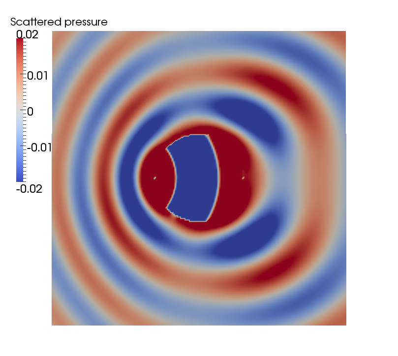
Consider an ellipsoid with major axis directed along the zz-axis. This object is included inside a larger ball. The external border of the ball after discretization is the surface Γ∞\Gamma_{\infty}. A potential flow is computed around the ellipsoid and inside the ball, such that the flow is uniform outside the ball, of Mach number 0.30.3 and directed along the zz-axis. An acoustic monopole source lies upstream of the ball, on the zz-axis as well. Four different meshes are considered, see Table 1. For accuracy reasons, a rule of thumb in boundary element methods for the classical Helmholtz equation is to set the mean edge length to a value eight to ten times smaller than the wavelength of the source. In our simulations, we first generate the mesh and then apply the Prandtl–Glauert transformation. With the present choice for the Mach number, the mesh is at most extended by a factor γ∞≈1.048\gamma_{\infty}\approx 1.048. Moreover, the integral operators are computed at the transformed wavenumber k^∞=γ∞​k∞≈0.21\hat{k}_{\infty}=\gamma_{\infty}k_{\infty}\approx 0.21 m. We then verify that, for Mesh 1, the mean length of the edges of the transformed mesh is eight times smaller than the wavelength. The three coarser meshes do not satisfy the rule of thumb and are used as comparison supports and in numerical experiments requiring a large number of resolutions.

From Table 1, for fine meshes, the number of basis functions used to discretize the unknown pp in the variational formulation (43) takes a smaller part in the total number of basis functions than for coarse meshes (from 20% down to 12%). Therefore, the relative complexity added to (42) by the third equation of (43) decreases with the total number of unknowns, which is an interesting property when it comes to industrial test cases. Figure 3 displays Mesh 1 and the rescaled velocity 𝑴0\boldsymbol{M}_{0} of the potential flow.

In what follows, a frequency 𝚏\mathtt{f} is called resonant if −k^∞2=−4​π2​𝚏2γ∞2∈Λ-\hat{k}_{\infty}^{2}=-\frac{4\pi^{2}\mathtt{f}^{2}}{\gamma_{\infty}^{2}}\in\Lambda, where Λ\Lambda is the set of Dirichlet eigenvalues for the Laplacian on ℝ3\Ω+¯\mathbb{R}^{3}\backslash\overline{\Omega^{+}}. The set Λ\Lambda depends on the shape of the coupling surface Γ∞\Gamma_{\infty}, which slightly changes after each discretization.

Mesh 1 Mesh 2 Mesh 3 Mesh 4
number of volumic dofs Φ\Phi 17961796 687687 194194 7979
number of surfacic ℙ0\mathbb{P}_{0} dofs λ\lambda 808808 510510 270270 148148
number of surfacic ℙ1\mathbb{P}_{1} dofs pp 406406 257257 137137 7676
proportion of dofs pp in the total number of dofs 11.9%11.9\% 15.0%15.0\% 18.6%18.6\% 20.0%20.0\%
smallest edge (mm) 7.097.09 8.788.78 15.7115.71 19.1819.18
mean edge (mm) 22.6422.64 32.2032.20 49.7849.78 66.4666.46
largest edge (mm) 56.8756.87 70.6270.62 103.59103.59 112.71112.71
Table 1: Characteristics of the four considered meshes.
Refer to caption
Refer to caption
Figure 3: Left: representation of Mesh 1, Right: potential flow around the ellipsoid.

6.1 Comparison of pressure fields

As seen in Theorem 4.2, the unstable formulation (42) is not well-posed at resonant frequencies. First, a prospective study to identify a resonant frequency for each of the four meshes is carried out by monitoring the condition number of the corresponding matrices. A resonant frequency for Mesh 1, Mesh 2, Mesh 3, and Mesh 4 is identified around 1509.8491509.849 Hz, 1513.4311513.431 Hz, 1521.0151521.015 Hz, and 1535.7041535.704 Hz, respectively.

The convergence of the iterative solver is monitored by requiring that the Euclidian norm of the relative residual is smaller than 10−610^{-6}. Additional tests indicate that the discretized solution to the stable formulation does not change much below this value of the relative residual. For Mesh 1, away from a resonance, say at 15001500 Hz, the scattered pressure fields computed with the unstable and stable formulations are very similar. This holds as well for the total pressure fields, see Figure 4. At the resonant frequency 1509.8491509.849 Hz, the unstable formulation (42) yields pressure maps quite different from the ones at 15001500 Hz, whereas the stable formulation (43) yields pressure maps very similar to the ones at 15001500 Hz, see Figure 5. The distortion of the scattered field with the unstable formulation (42) is the result of the significant magnification of numerical errors by the ill-conditioning of the linear system approximating (42).

Refer to caption
Refer to caption
Refer to caption
Refer to caption
Figure 4: Mesh 1, 15001500 Hz. Top : real part of the total pressure; left: unstable formulation (42), right: stable formulation (43). Bottom : real part of the scattered pressure; left: unstable formulation (42), right: stable formulation (43). At this non-resonant frequency, both formulations yield similar results.
Refer to caption
Refer to caption
Refer to caption
Refer to caption
Figure 5: Mesh 1, 1509.8491509.849 Hz. Top : real part of the total pressure; left: unstable formulation (42), right: stable formulation (43). Bottom : real part of the scattered pressure; left: unstable formulation (42), right: stable formulation (43). At this resonant frequency, the two formulations yield different results.

6.2 Auxiliary variable pp

In Figure 6, the left plot indicates that with Mesh 1, the magnitude of pp is around 0.5%0.5\% of the scattered pressure. The right plot shows the behaviour of the magnitude of pp (measured as ‖p‖L∞​(Γ∞)\|p\|_{L^{\infty}(\Gamma_{\infty})}) with respect to the stopping criterion of the iterative solver for the four meshes. The finer the mesh, the smaller the auxiliary variable pp, which is consistent with the fact that the pp-component of the solution to (43) vanishes (see Section 4.4).

Refer to caption
10−610^{-6}10−510^{-5}10−410^{-4}10−310^{-3}10−210^{-2}10−110^{-1}10−410^{-4}10−310^{-3}10−210^{-2}10−110^{-1}stopping criterion of the iterative solvermagnitude of the auxiliary variable ppMesh 1Mesh 2Mesh 3Mesh 4
Figure 6: Stable formulation (43) at 15001500 Hz. Left : real part of the scattered pressure and auxiliary variable pp with Mesh 1. Right : Magnitude of the auxiliary variable pp as a function of the stopping criterion of the iterative linear solver with all meshes.

6.3 Comparison of condition numbers

Figure 7 presents the condition numbers of the matrices resulting from the formulations (42) and (43) as a function of the frequency. In the left plot, the curves are centered at the resonant frequencies. The finer the mesh, the higher the condition number explodes. The width of the peak at the resonance does not appear to depend on the mesh. In the right plot, a larger frequency bandwidth is considered with Mesh 22. Owing to the frequency sampling (every 55 Hz), some resonances may be missed, and the local maxima may not be accurately reached (in particular, from the left plot, the local maximum of 7.27.2 for log(cond(MM)) at 1513.4311513.431 Hz is very underestimated). The stable formulation (43) produces somewhat larger condition numbers for the large majority of the frequencies, but, unlike the unstable formulation (42), it presents no resonance. Moreover, from the Weyl formula, the number of resonant frequencies smaller than 𝚏\mathtt{f} increases as 𝚏32\mathtt{f}^{\frac{3}{2}}, making the need for a stable formulation even more important for simulations at higher frequencies.

−5-5005510310^{3}10610^{6}10910^{9}distance to resonant frequency (Hz)cond(AunstabA^{\rm unstab}), cond(AstabA^{\rm stab})Mesh 1Mesh 2Mesh 3Mesh 4
1,5001{,}5002,0002{,}0002,5002{,}5003,0003{,}00010210^{2}10310^{3}10410^{4}10510^{5}frequency (Hz)cond(AunstabA^{\rm unstab}), cond(AstabA^{\rm stab})unstable formulation (42)stable formulation (43)
Figure 7: Condition number of the matrix for the unstable formulation (42) (solid) and the stable formulation (43) (dashed). Left: centered representation around a resonant frequency for the four meshes. Right: larger bandwidth with Mesh 2.

6.4 Convergence

To further study the impact of the ill-conditioning of the unstable formulation (42) on the computed solution, the preconditioning is not used in what follows. First, the value of the acoustic pressure on a network of 1000010000 points located further than 0.50.5 m from the center of the sphere (therefore in Ω+\Omega^{+}) is computed using the stable formulation (43) with Mesh 1 at the resonant frequency 1509.8491509.849 Hz. This computed acoustic pressure is called the accurate pressure. Next, the acoustic pressure on the same network of points is computed for different values of the number of iterations of the solver, using the unstable formulation (42) and the stable formulation (43) with Mesh 1 at the same frequency. The relative difference between the computed pressure and the accurate pressure in Euclidian norm is called the relative error. Figure 8 presents the relative residual and the relative error with respect to the number of iterations. With the unstable formulation (42), the relative residual decreases irregularly. In particular, it stays constant during around 200200 iterations. The relative error decreases, stays constant, rises after 400400 iterations, and finally stabilizes at a large value, whereas the relative residual keeps converging to zero. As for every ill-conditioned problem, the relative residual cannot be used to ascertain convergence towards the correct solution. In particular, after 600600 iterations, the relative residual is extremely small, while the error is of order one. With the stable formulation (43), the relative residual and the relative error decrease regularly, and in the same fashion.

0020020040040060060010−710^{-7}10−410^{-4}10−110^{-1}number of iterationsrelative residualunstable formulation (42)stable formulation (43)
0020020040040060060010−310^{-3}10−110^{-1}10110^{1}number of iterationsrelative errorunstable formulation (42)stable formulation (43)
Figure 8: Mesh 1 at resonance 1509.8491509.849 Hz; relative residual (left) and relative error (right) with respect to the number of iterations.

6.5 Choice of the coupling parameter η\eta

In the stable formulation (43), the choice of the coupling parameter η\eta is expected to have a direct effect of the condition number of the matrix AstabA^{\rm stab}. In Figure 9, this condition number is plotted for Mesh 4 and for various values of η\eta. For η=0\eta=0, equations (43a)-(43b) are decoupled from (43c), and (43a)-(43b) become (42), so that the curve for η=0.001\eta=0.001 is similar to the curve of the unstable formulation for Mesh 4 in Figure 7. The condition number appears to be the smallest for η\eta in the range 1 to 10, and worsens for lower and higher values of η\eta. This motivates the choice η=1\eta=1 made in the above simulations.

−5-5005510310^{3}10410^{4}10510^{5}10610^{6}distance to resonant frequency (Hz)cond(AstabA^{\rm stab})η=0.001\eta=0.001η=0.01\eta=0.01η=0.1\eta=0.1η=1\eta=1η=10\eta=10η=100\eta=100
Figure 9: Condition number of the matrix for the stable formulation (43) centered around the resonant frequency at 1535.7041535.704 Hz for Mesh 4. In this case, the chosen value η=1\eta=1 leads to the minimal condition numbers.

7 Conclusion

In this work, we derived two coupled formulations for the convected Helmholtz equation with non-uniform flow in a bounded domain. The first formulation involves one surface unknown and is well-posed except at some resonant frequencies of the source, while the second formulation is unconditionally well-posed and involves two surface unknowns. Our numerical results show that at resonant frequencies, the discretization of the first formulation is ill-conditioned so that the pressure field is plagued by spurious oscillations. Moreover, the second formulation remains tractable within large industrial problems since the relative complexity added by the second surface unknown decreases with the size of the mesh. The interest in the second formulation is also enhanced by the fact that, at higher frequencies, the density of resonant frequencies is more important.

As long as the uniform flow assumption in the exterior domain is reasonable, more complex flows in the interior domain can be considered, as well as more complex boundary conditions at the surface of the scattering object. These extensions only require to modify the finite element part of the present methodology.

Another interesting extension of this work is the resolution of parametrized aeroacoustic problems, with the frequency of the source as a parameter, using reduced-order models, for instance by means of Proper Generalized Decomposition or Reduced Basis methods. Using the first formulation may involve ill-conditioned numerical resolutions if the frequency range of interest contains resonant frequencies, whereas the second formulation guarantees well-posedness of the procedure. Moreover, the complexity of the online stage of the reduced-order model is not increased when using the second formulation.

Acknowledgement

This work was partially supported by EADS Innovation Works. The authors thank Toufic Abboud (IMACS), Nolwenn Balin (EADS Innovation Works), François Dubois (CNAM), Patrick Joly (INRIA), and Tony Lelièvre (CERMICS) for fruitful discussions.

References

  • [1] P.R. Amestoy, I.S. Duff, and J.-Y. L’Excellent. Multifrontal parallel distributed symmetric and unsymmetric solvers. Comput. Methods Appl. Mech. Engrg., 184(2–4):501–520, 2000.
  • [2] R. Amiet and W. R. Sears. The aerodynamic noise of small-perturbation subsonic flows. J. Fluid Mech., 44:227–235, 1928.
  • [3] E. Bécache, A. S. Bonnet-Ben Dhia, and G. Legendre. Perfectly matched layers for the convected Helmholtz equation. SIAM J. Numer. Anal., 42(1):409–433, 2004.
  • [4] M. Beldi and A. Maghrebi. Some new results for the study of acoustic radiation within a uniform subsonic flow using boundary integral method. Advanced Materials Research, 488–489:383–395, 2012.
  • [5] P. Bettess. Infinite Elements. Penshaw Press: Cleadon, Sunderland, U.K., 1992.
  • [6] H. Brakhage and P. Werner. Über das Dirichletsche Außenraum Problem für die Helmholtzsche Schwingungsgleichung. Arch. der Math., 16:325–329, 1965.
  • [7] S.C. Brenner and L.R. Scott. The Mathematical Theory of Finite Element Methods, volume 15 of Texts in Applied Mathematics. Springer, 2008.
  • [8] A. Buffa and R. Hiptmair. Regularized combined field integral equations. Numer. Math., 100(1):1–19, 2005.
  • [9] B. Carpentieri. Sparse preconditioners for dense linear systems from electromagnetic applications. PhD thesis, CERFACS, 2002.
  • [10] B. Carpentieri, I. Duff, L. Giraud, and G. Sylvand. Combining fast multipole techniques and an approximate inverse preconditioner for large electromagnetism calculations. SIAM J. Sci. Comput., 27(3):774–792, 2005.
  • [11] C. Carstensen, S.A. Funken, and E.P. Stephan. On the adaptive coupling of FEM and BEM in 2-D-elasticity. Numer. Math., 77(2):187–221, 1997.
  • [12] M. Costabel. Symmetric methods for the coupling of finite elements and boundary elements, volume 1 of Boundary Elements IX. Springer-Verlag, Berlin, 1987.
  • [13] C. Domínguez, E.P. Stephan, and M. Maischak. FE/BE coupling for an acoustic fluid-structure interaction problem. Residual a posteriori error estimates. Internat. J. Numer. Methods Engrg., 89(3):299–322, 2012.
  • [14] F. Dubois, E. Duceau, F. Maréchal, and I. Terrasse. Lorentz transform and staggered finite differences for advective acoustics. Technical report, EADS, 2002.
  • [15] A. Ern and J.L. Guermond. Theory and Practice of Finite Elements, volume 159 of Applied Mathematical Sciences. Springer, 2004.
  • [16] G. Fairweather, A. Karageorghis, and P.A. Martin. The method of fundamental solutions for scattering and radiation problems. Eng. Anal. Bound. Elem., 27(7):759–769, 2003.
  • [17] N. Garofalo and F.-H. Lin. Unique continuation for elliptic operators: A geometric-variational approach. Comm. Pure Appl. Math., 40(3):347–366, 1987.
  • [18] H. Glauert. The effect of compressibility on the lift of an aerofoil. Proc. R. Soc. Lond. Ser. A Math. Phys. Eng. Sci., 118(779):113–119, 1928.
  • [19] M.E. Goldstein. Aeroacoustics. McGraw-Hill International Book Company, 1976.
  • [20] M.F. Hamilton and D.T. Blackstock. Nonlinear Acoustics: Theory and Applications. Elsevier Science & Tech, 1998.
  • [21] R. Hiptmair. Coupling of finite elements and boundary elements in electromagnetic scattering. SIAM J. Numer. Anal., 41(3):919–944, 2003.
  • [22] R. Hiptmair and P. Meury. Stabilized FEM-BEM coupling for Helmholtz transmission problems. SIAM J. Numer. Anal., 44(5):2107–2130, 2006.
  • [23] A. Hirschberg and S. W. Rienstra. An Introduction to Acoustics. Eindhoven University of Technology, 2004.
  • [24] G. C. Hsiao and W. L. Wendland. Boundary Element Methods: Foundation and Error Analysis. John Wiley & Sons, Ltd, 2004.
  • [25] J.M. Jin and V.V. Liepa. A note on hybrid finite element method for solving scattering problems. IEEE Trans. Ant. Prop., 36(10):1486–1490, 1988.
  • [26] C. Johnson and J. C. Nédélec. On the coupling of boundary integral and finite element methods. Math. Comp., 35(152):1063–1079, 1980.
  • [27] J. Langou. Solving large linear systems with multiple right-hand sides. PhD thesis, INSA, 2003.
  • [28] R. Leis. Zur Dirichletschen Randwertaufgabe des Außenraumes der Schwingungsgleichung. Math. Z., 90:205–211, 1965.
  • [29] V. Levillain. Couplage éléments finis-équations intégrales pour la résolution des équations de Maxwell en milieu hétèrogène. PhD thesis, École Polytechnique, 1991.
  • [30] F. Leydecker, M. Maischak, E.P. Stephan, and M. Teltscher. Adaptive FE-BE coupling for an electromagnetic problem in ℝ3\mathbb{R}^{3}—a residual error estimator. Math. Methods Appl. Sci., 33(18):2162–2186, 2010.
  • [31] M. J. Lighthill. On sound generated aerodynamically. I. General theory. Proc. R. Soc. Lond. Ser. A Math. Phys. Eng. Sci., 211(1107):564–587, 1952.
  • [32] M. J. Lighthill. On sound generated aerodynamically. II. Turbulence as a source of sound. Proc. R. Soc. Lond. Ser. A Math. Phys. Eng. Sci., 222(1148):1–32, 1954.
  • [33] M. Maischak and E.P. Stephan. A FEM-BEM coupling method for a nonlinear transmission problem modelling coulomb friction contact. Comput. Methods Appl. Mech. Engrg., 194(2-5):453–466, 2005.
  • [34] B. McDonald and A. Wexler. Finite-element solution of unbounded field problems. IEEE Trans. Microwave Theory Tech., 20(12):841–847, 1972.
  • [35] W. McLean. Strongly Elliptic Systems and Boundary Integral Equations. Cambridge University Press, 2000.
  • [36] D. Mitsoudis, C. Makridakis, and M. Plexousakis. Helmholtz equation with artificial boundary conditions in a two-dimensional waveguide. SIAM J. Math. Anal., 44(6):4320–4344, 2012.
  • [37] D.P. O’Leary. The block conjugate gradient algorithm and related methods. Linear Algebra Appl., 29:293–322, 1980.
  • [38] O. Panich. On the question of solvability of the exterior boundary value problems for the wave equation and Maxwell’s equations. Russian Math. Surv., 20:221–226, 1965.
  • [39] C. J. Powles and B. J. Tester. Asymptotic and numerical solutions for shielding of noise sources by parallel coaxial jet flows. In 14th AIAA/CEAS Aeroacoustics Conference, 2008.
  • [40] Y. Saad and M. Schultz. GMRES: A generalized minimal residual algorithm for solving nonsymmetric linear systems. SIAM J. Sci. and Stat. Comput., 7(3):856–869, 1986.
  • [41] S.A. Sauter and C. Schwab. Boundary Element Methods, volume 39 of Springer Series in Computational Mathematics. Springer, 2010.
  • [42] L. Tartar. An Introduction to Sobolev Spaces and Interpolation Spaces, volume 3 of Lecture Notes of the Unione Matematica Italiana. Springer, 2007.
  • [43] J. Utzmann, C.-D. Munz, M. Dumbser, E. Sonnendrücker, S. Salmon, S. Jund, and E. Frénod. Numerical Simulation of Turbulent Flows and Noise Generation. Springer, 2009.
  • [44] O. von Estorff and M. Firuziaan. Coupled BEM/FEM approach for nonlinear soil/structure interaction. Eng. Anal. Bound. Elem., 24(10):715–725, 2000.
  • [45] O. C. Zienkiewicz, D. W. Kelly, and P. Bettess. The coupling of the finite element method and boundary solution procedures. Int. J. Numer. Meth. Engng., 11:355–375, 1977.
  • [46] O.C. Zienkiewicz and P. Bettess. Fluid-structure dynamic interaction and wave forces. An introduction to numerical treatment. Int. J. Numer. Meth. Engng., 13(1):1–16, 1978.