Sharp regularity near an absorbing boundary for solutions to second order SPDEs in a half-line with constant coefficients

Sean Ledger Address: Mathematical Institute, University of Oxford, Woodstock Road, Oxford, OX2 6GG Email address: ledger@maths.ox.ac.uk

Abstract.

We prove that the weak version of the SPDE problem

	$\displaystyle dV_{t}(x)$	$\displaystyle=[-\mu V_{t}^{\prime}(x)+\frac{1}{2}(\sigma_{M}^{2}+\sigma_{I}^{2})V_{t}^{\prime\prime}(x)]dt-\sigma_{M}V_{t}^{\prime}(x)dW^{M}_{t},\quad x>0,$
	$\displaystyle V_{t}(0)$	$\displaystyle=0$

with a specified bounded initial density, $V_{0}$ , and $W$ a standard Brownian motion, has a unique solution in the class of finite-measure valued processes. The solution has a smooth density process which has a probabilistic representation and shows degeneracy near the absorbing boundary. In the language of weighted Sobolev spaces, we describe the precise order of integrability of the density and its derivatives near the origin, and we relate this behaviour to a two-dimensional Brownian motion in a wedge whose angle is a function of the ratio $\sigma_{M}/\sigma_{I}$ . Our results are sharp: we demonstrate that better regularity is unattainable.

1. Introduction

Let $W$ be a standard Brownian motion on a complete filtered probability space $\left(\Omega,\mathcal{F},\mathbf{P}\right)$ and $V_{0}$ be a deterministic bounded probability density function on the half-line $\left(0,\infty\right)$ . In this paper, we consider the problem of finding a finite-measure valued process, $\nu=\left(\nu_{t}\right)_{t\in\left[0,T\right]}$ , satisfying the weak stochastic partial differential equation

(1.1)

\left\langle\phi,\nu_{t}\right\rangle=\left\langle\phi,V_{0}\right\rangle+\int_{0}^{t}[\mu\left\langle\phi^{\prime},\nu_{s}\right\rangle+\frac{1}{2}(\sigma_{M}^{2}+\sigma_{I}^{2})\left\langle\phi^{\prime\prime},\nu_{s}\right\rangle]ds+\sigma_{M}\int_{0}^{t}\left\langle\phi^{\prime},\nu_{s}\right\rangle dW_{s}

for all $t\in\left[0,T\right]$ and $\phi\in C^{\textrm{test}}$ . Here, we use the abbreviation $\left\langle\phi,\nu_{t}\right\rangle=\int_{0}^{\infty}\phi(x)\nu_{t}(dx)$ and write $C^{\textrm{test}}$ for the space of bounded, twice-differentiable functions that vanish at the origin and have bounded first and second derivatives. The coefficients $\mu\in\mathbf{R}$ , $\sigma_{M}>0$ , and $\sigma_{I}>0$ and the time horizon $T>0$ are deterministic constants. We prove this problem has a unique solution, show how to construct this solution, and establish its regularity near the absorbing boundary.

This stochastic partial differential equation (SPDE) arises naturally as the mean-field limit of a collection of interacting particles. Specifically, suppose we have a homogeneous pool of particles each experiencing an independent noise driven by a Brownian motion with speed $\sigma_{I}$ and drift $\mu$ , as well as a common noise $\sigma_{M}W_{t}$ . If we kill each of the particles upon hitting the origin, then $\nu_{t}$ describes the limiting spatial distribution of the particles at time $t$ as the number of particles becomes large. In [BHH+11], this model is proposed for the pricing of portfolio credit derivatives, and in that context the common noise, $W$ , corresponds to a market risk factor and the event that a particle hits the origin represents a default of one of the names in the portfolio. As the particles in this model are independent and identically distributed conditional on knowing the history of $W$ , we can study the system by considering the conditional mean behaviour of a single particle. In Section 2 we use this idea to present a simple construction of the solution to (1.1).

Visualising the dynamics of the solution to (1.1) is straightforward, and if $\sigma_{M}=0$ then the SPDE becomes the deterministic heat equation with zero boundary condition. For non-zero $\sigma_{M}$ the solution still has this decay, but also experiences random fluctuations in location which are driven by the Brownian motion $W$ — see Figure 1. If we denote the density of the solution by $V$ , then we can write (1.1) in differential form:

dV_{t}=[-\mu V_{t}^{\prime}+\frac{1}{2}(\sigma_{M}^{2}+\sigma_{I}^{2})V_{t}^{\prime\prime}]dt-\sigma_{M}V_{t}^{\prime}dW_{t},

and, thinking of this equation as a PDE with irregular coefficients, we see that $V$ diffuses with speed $\sigma_{M}^{2}+\sigma_{I}^{2}$ and the transport term, $\mu dt+\sigma_{M}dW_{t}$ , describes the (stochastic) net movement of the density in space. Lemma 3.1 of [Kry03] shows that the density of the solution is infinitely differentiable in $\left(0,\infty\right)$ , and this is due to the smoothing effect that heat flow produces. However, the presence of the irregular fluctuations in the density’s location causes mass close to the boundary to be destroyed in an abrupt fashion, and as a result the derivatives of the density blow-up at the origin. The purpose of this paper is to describe this degeneracy at the absorbing boundary.

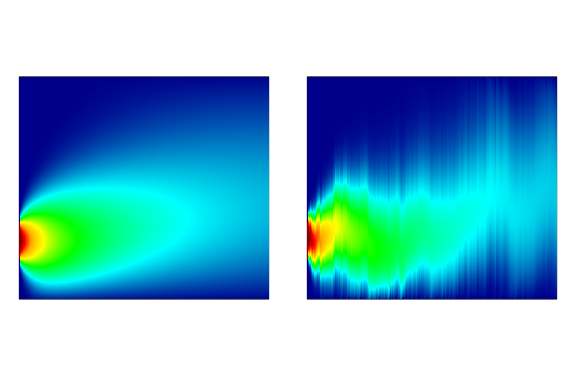
Refer to caption — Figure 1.1. On the left is the evolution of the system in the deterministic case $\sigma_{M}=0$ . The value of the density at a space-time point is represented by a colour increasing from blue ( $V_{t}\left(x\right)=0$ ) through to red ( $V_{t}\left(x\right)=1$ ). The initial condition is the step function $V_{0}=\mathbf{1}_{\left(0.18,0.5\right)}$ and the drift, $\mu$ , is zero. Compare this with a realisation of the evolution for same parameters but with $\sigma_{M}>0$ , which is presented on the right. We still observe heat-type dispersion but with a non-smooth fluctuation in the density’s location.

Dirichlet boundary problems for SPDEs of this type have been studied extensively — for example [KK04, Kry94, KL98]. As we are working in one-dimension with constant coefficients, the simplicity of our setting allows greater insight into the behaviour of the solution near the absorbing boundary. We take advantage of a straightforward smoothing technique to present a more elementary study of the problem than is currently offered in the standard literature, and we are able to prove uniqueness of the solution to (1.1) in the broad class of finite-measure valued processes. Throughout this paper, when referring to uniqueness we shall always mean that if $\nu^{1}$ and $\nu^{2}$ are two finite-measure valued processes solving (1.1), then

\mathbf{E}\int_{0}^{T}\left(\left\langle\phi,\nu_{t}\right\rangle-\left\langle\phi,\bar{\nu}_{t}\right\rangle\right)^{2}dt=0,\quad\mathrm{for\,every}\,\phi\in C^{\textrm{test}}.

The results closest to those in this paper are found in [Kry94]; there, Krylov demonstrates the existence of a unique solution to (1.1) in the class of twice-differentiable function-valued processes, $U=\left(U_{t}\left(x\right)\right)_{t\in\left[0,T\right]}$ , that satisfy

\mathbf{E}\int_{0}^{T}\bigl(\left\|U_{t}\right\|_{L^{2}\left(0,\infty\right)}^{2}+\left\|U_{t}^{\prime}\right\|_{L^{2}\left(0,\infty\right)}^{2}+\left\|xU_{t}^{\prime\prime}\right\|_{L^{2}\left(0,\infty\right)}^{2}\bigr)dt<\infty.

Furthermore, Krylov shows that if the initial density is $N$ -times differentiable with the function $x\mapsto x^{k}V_{0}^{\left(k\right)}\left(x\right)$ in $L^{2}\left(0,\infty\right)$ for $k=0,1,\ldots,N$ , then the solution is $\left(N+1\right)$ -times differentiable with

(1.2)

\mathbf{E}\int_{0}^{T}\bigl\|x^{k-1}U_{t}^{\left(k\right)}\bigr\|_{L^{2}\left(0,\infty\right)}^{2}dt<\infty

for $k=0,1,\ldots,N+1$ . (For a function $f$ on $\left(0,\infty\right)$ , we will always denote the $n^{\mathrm{th}}$ order derivative of $f$ by $f^{\left(n\right)}$ .)

A key ingredient in [Kry94], and the majority of the literature on this problem, is the introduction of weighted Sobolev spaces. These spaces enable us to quantify the rate at which the solution and its derivatives blow-up near the origin. In our one-dimensional setting, it suffices to use the functions

(1.3)

w_{c}\left(x\right):=x^{c}e^{-x},\quad x>0,

for $c\in\mathbf{R}$ . For a given order of derivative of the solution to (1.1), we can ask: how small can $c$ be taken in the above weighting function whilst preserving square-integrability of the product of that derivative and $w_{c}$ ? From (1.2), we can certainly take any $c\geq k-1$ for the $k^{\mathrm{th}}$ derivative of the solution. A complete answer to this question is provided by the two proceeding theorems, and a critical quantity is

(1.4)

\alpha:=\frac{\pi}{2}+\arcsin\rho\in\left(\pi/2,\pi\right),\quad\textrm{where }\,\rho:=\frac{\sigma_{M}}{\sqrt{\sigma_{M}^{2}+\sigma_{I}^{2}}}\in\left(0,1\right).

In the context of credit derivatives, $\rho$ is referred to as the correlation in the portfolio and describes the tendency of defaults to occur simultaneously. The closer $\rho$ is to one, the larger the value of $\alpha$ , and therefore, observing that $\pi/\alpha-1\in\left(0,1\right)$ , the following result states that higher correlation produces less regularity near the absorbing boundary.

Theorem 1.1 (Uniqueness and regularity).

If $V_{0}$ is bounded, then there exists a unique solution, $\nu$ , to (1.1) in the class of finite-measure valued processes, and, for almost every $\left(\omega,t\right)\in\Omega\times\left[0,T\right]$ , $\nu_{t}$ has a density $V_{t}$ on $\left(0,\infty\right)$ .

Furthermore, suppose that $V_{0}$ is $N$ -times weakly differentiable in $\left(0,\infty\right)$ , and that for $k=0,1,\ldots,N$

\bigl\|w_{k-\beta/2}V_{0}^{\left(k\right)}\bigr\|_{L^{2}\left(0,\infty\right)}<\infty,\quad\textrm{for every }\beta\in\left(-\infty,\pi/\alpha-1\right),

where $w_{\left(\cdot\right)}$ and $\alpha$ are defined in (1.3) and (1.4). Then, for almost all $\left(\omega,t\right)\in\Omega\times\left[0,T\right]$ , $V_{t}$ is $\left(N+1\right)$ -times weakly differentiable in $\left(0,\infty\right)$ , and for $k=0,1,\ldots,N+1$

\mathbf{E}\int_{0}^{T}\bigl\|w_{k-1-\beta/2}V_{t}^{\left(k\right)}\bigr\|_{L^{2}\left(0,\infty\right)}^{2}dt<\infty,\quad\textrm{for every }\beta\in\left(-\infty,\pi/\alpha-1\right).

This result shows that, at a time later than zero, the solution has differentiability one order higher than the initial density, and is one multiple of $x$ more regular at the origin (recall that $w_{k-\beta/2}\left(x\right)=x^{k-\beta/2}e^{-x}$ ). We should notice that, because the initial density is integrable and bounded, the condition $w_{-\beta/2}V_{0}\in L^{2}\left(0,\infty\right)$ is always satisfied. The hypotheses placed on the initial density allow its derivatives to blow-up at the origin and grow sub-exponentially towards infinity. We recover the results of [Kry94] by taking $\beta=0$ in Theorem 1.1, and therefore we have expanded upon the known regularity of the solution near the absorbing boundary.

Our results are sharp as the following result shows that we cannot take $\beta>\pi/\alpha-1$ in Theorem 1.1:

Theorem 1.2 (Converse result).

If $V_{0}$ satisfies the hypotheses of Theorem 1.1, then for $k=0,1,\ldots,N+1$ we have

\mathbf{E}\int_{0}^{T}\bigl\|w_{k-1-\beta/2}V_{t}^{\left(k\right)}\bigr\|_{L^{2}\left(0,\infty\right)}^{2}dt=\infty,\quad\textrm{for every }\beta\in\left(\pi/\alpha-1,+\infty\right).

Since the tails of the weighting functions all decay at the same rate, the only way we can obtain the blow-up observed in Theorem 1.2 is if the solution is degenerate near the absorbing boundary. With this in mind, it is clear that the first derivative of the solution cannot be bounded in a neighbourhood of the origin, otherwise we obtain the contradiction

\int_{0}^{1}x^{-\beta}dx=\infty

for $\beta\in\left(\pi/\alpha-1,1\right)\subseteq\left(0,1\right)$ . In the deterministic setting ( $\sigma_{M}=0$ ) the first derivative does not have this feature, and this has been remarked upon by Krylov in [Kry03]. If we shift the density by setting

f\left(t,x\right):=V_{t}\left(x+\mu t+\sigma_{M}W_{t}\right),

then, by the Itō–Wentzell formula, we have that $f$ solves the deterministic heat equation (with speed $\sigma_{I}$ ) in the random region

\left\{\left(t,x\right):t\in\left[0,T\right],x>-\mu t-\sigma_{M}W_{t}\right\}

with Dirichlet boundary condition. Theorem 5.1 of [Kry03] shows that there exists $\lambda\in\left(0,1\right)$ such that, with probability one, there is a dense subset of $\left[0,T\right]$ on which

\lim_{x\downarrow 0}\frac{f\left(t,x\right)}{x^{\lambda}}=\infty.

On this set it is clear that the density can have no spatial derivative at the absorbing boundary.

In the next section we present the construction of the solution to (1.1) and describe its properties. A proof of Proposition 2.7 is presented in Section 3, and this is the main probabilistic result used to prove the above two theorems in Sections 4 and 5.

Acknowledgements

I would like to thank Ben Hambly for introducing me to this problem and related models, and Philippe Charmoy and James Leahy for helpful conversations.

2. The probabilistic solution

We shall construct the solution to (1.1) in this section. We have not yet proved that (1.1) can admit only one solution, therefore we refer to the measure-valued process presented here as the probabilistic solution.

Construction

Let us introduce two independent standard Brownian motions, $W^{1}$ and $W^{2}$ , that are also independent of $W$ . We define two test processes, $X^{1}$ and $X^{2}$ , by

X_{t}^{i}:=X_{0}^{i}+\mu t+\sigma_{M}W_{t}+\sigma_{I}W_{t}^{i},

where $X_{0}^{1}$ and $X_{0}^{2}$ are independent random variables with common law $V_{0}$ , and are also independent of every other random variable introduced so far. To kill the particles upon hitting zero, we set

\tau^{i}:=\inf\left\{s\in\left[0,T\right]:X_{s}^{i}\leq 0\right\}.

Conditional on knowing the trajectory of $W$ , $X^{1}$ and $X^{2}$ are independent and identically distributed, therefore we make the following definition:

Definition 2.1 (Probabilistic solution).

Let $\mathcal{F}^{W}=\left\{\mathcal{F}_{t}^{W}\right\}_{t\in\left[0,T\right]}$ be the natural filtration of $W$ . The probabilistic solution, $\nu$ , is defined to be the measure-valued process

\nu_{t}\left(S\right):=\mathbf{P}\left(\left.X_{t}^{1}\in S;t<\tau^{1}\right|\mathcal{F}_{t}^{W}\right)

for all $t\in\left[0,T\right]$ and $S\subseteq\left(0,\infty\right)$ Lebesgue measurable.

Throughout this paper “ $S\subseteq\left(0,\infty\right)$ measurable” shall always mean that $S$ is Lebesgue measurable. The following is a useful representation:

Proposition 2.2.

For all $t\in\left[0,T\right]$ and $S\subseteq\left(0,\infty\right)$ measurable we have

\mathbf{E}\left[\nu_{t}\left(S\right)^{2}\right]=\mathbf{E}\left[\mathbf{E}\left[\left.\mathbf{1}_{X_{t}^{1}\in S,\,X_{t}^{2}\in S};t<\min\left(\tau^{1},\tau^{2}\right)\right|\mathcal{F}_{t}^{W}\right]\right]\!.

Proof.

Since $X^{1}$ and $X^{2}$ are equal in distribution, we have $\nu_{t}\left(S\right)=\mathbf{E}\left[\left.\mathbf{1}_{X_{t}^{i}\in S};t<\tau^{i}\right|\mathcal{F}_{t}^{W}\right]$ for $i=1$ and $2$ . Hence

	$\displaystyle\mathbf{E}\left[\nu_{t}\left(S\right)^{2}\right]$	$\displaystyle=\mathbf{E}\left[\mathbf{E}\left[\left.\mathbf{1}_{X_{t}^{1}\in S};t<\tau^{1}\right\|\mathcal{F}_{t}^{W}\right]^{2}\right]$
		$\displaystyle=\mathbf{E}\left[\mathbf{E}\left[\left.\mathbf{1}_{X_{t}^{1}\in S};t<\tau^{1}\right\|\mathcal{F}_{t}^{W}\right]\mathbf{E}\left[\left.\mathbf{1}_{X_{t}^{2}\in S};t<\tau^{2}\right\|\mathcal{F}_{t}^{W}\right]\right]$
		$\displaystyle=\mathbf{E}\left[\mathbf{E}\left[\left.\mathbf{1}_{X_{t}^{1}\in S,\,X_{t}^{2}\in S};t<\min\left(\tau^{1},\tau^{2}\right)\right\|\mathcal{F}_{t}^{W}\right]\right]$

as required, where the final line is due to the conditional independence of $X^{1}$ and $X^{2}$ . ∎

It is a simple calculation with Itō’s formula to show that $\nu$ is a solution of (1.1):

Proposition 2.3.

There exists a full subset of $\Omega$ on which

\left\langle\phi,\nu_{t}\right\rangle=\left\langle\phi,V_{0}\right\rangle+\int_{0}^{t}[\mu\left\langle\phi^{\prime},\nu_{s}\right\rangle+\frac{1}{2}(\sigma_{M}^{2}+\sigma_{I}^{2})\left\langle\phi^{\prime\prime},\nu_{s}\right\rangle]ds+\sigma_{M}\int_{0}^{t}\left\langle\phi^{\prime},\nu_{s}\right\rangle dW_{s},

for all $t\in\left[0,T\right]$ and $\phi\in C^{\textrm{test}}$ .

Proof.

Take $\phi\in C^{\textrm{test}}$ , then Itō’s formula gives

(2.1)		$\displaystyle\phi(X_{t\wedge\tau^{1}}^{1})$	$\displaystyle=\phi(X_{0}^{1})+\int_{0}^{t}[\mu\phi^{\prime}(X_{s}^{1})+\frac{1}{2}(\sigma_{M}^{2}+\sigma_{I}^{2})\phi^{\prime\prime}(X_{s}^{1})]\mathbf{1}_{s<\tau^{1}}ds$
		$\displaystyle+\sigma_{M}\int_{0}^{t\wedge\tau^{1}}\phi^{\prime}(X_{s}^{1})\mathbf{1}_{s<\tau^{1}}dW_{s}+\sigma_{I}\int_{0}^{t\wedge\tau^{1}}\phi^{\prime}(X_{s}^{1})\mathbf{1}_{s<\tau^{1}}dW_{s}^{1}.$

Since $\phi(0)=0$ , we can write $\phi(X_{t\wedge\tau^{1}}^{1})=\phi(X_{t}^{1})\mathbf{1}_{t<\tau^{1}}$ , and therefore, by taking the conditional expectation over (2.1) and noting that the $W^{1}$ integral then vanishes, we arrive at the required result. ∎

Remark 2.4 (The choice of test functions).

$C^{\mathrm{test}}$ is chosen as it is the largest space for which the previous proof remains valid. The test functions’ derivatives need not be controlled at the origin, and we cannot take $C^{\mathrm{test}}=C_{0}^{\infty}(0,\infty)$ — the space of compactly supported smooth functions on the half-line — because in section 4 it will be necessary to set $T_{\delta}\phi$ (see Definition 4.1) into (1.1) despite the fact that in general $\left(T_{\delta}\phi\right)^{\prime}\left(0\right)$ and $\left(T_{\delta}\phi\right)^{\prime\prime}\left(0\right)$ are non-zero.

Remark 2.5 (Connection with filtering).

If we treat $X^{1}$ as a signal process and $W$ an observation process, then the Zakai equation (see for example [BC09]) for the conditional distribution of the signal given the observations is exactly (1.1).

2.1. Properties

Conditional on knowing $\mathcal{F}_{t}^{W}$ , the process $X^{1}$ is a Brownian motion started at $X_{0}^{1}$ with drift $t\mapsto\mu t+\sigma_{M}W_{t}$ , and therefore we can write the conditional density of $X^{1}$ as

P_{t}\left(x;x_{0}\right)=P_{t}\left(x;x_{0}\right)\left(\omega\right):=\frac{1}{\sqrt{2\pi\sigma_{I}^{2}t}}\exp\left\{-\frac{\left(x-x_{0}-\mu t-\sigma_{M}W_{t}\right)^{2}}{2\sigma_{I}^{2}t}\right\}.

From Definition 2.1, it is a trivial fact that $\nu_{t}\left(S\right)\leq\mathbf{P}\left(\left.X_{t}^{1}\in S\right|\mathcal{F}_{t}^{W}\right)$ for any time $t\in\left[0,T\right]$ and measurable subset $S\subseteq\left(0,\infty\right)$ , and this simple observation allows us to show that $\nu$ has a density process:

Proposition 2.6 (Existence of the density).

There exists a full subset of $\Omega$ on which, for every $t\in\left[0,T\right]$ , $\nu_{t}$ has a density process $V_{t}$ , and, for every $1\leq p\leq\infty$ , $V_{t}\in L^{p}\left(0,\infty\right)$ and $\left\|V_{t}\right\|_{p}\leq\left\|V_{0}\right\|_{p}$ .

Proof.

From the above, there exists a full subset of $\Omega$ on which

\nu_{t}\left(S\right)\leq\mathbf{P}\left(\left.X_{t}^{1}\in S\right|\mathcal{F}_{t}^{W}\right)=\int_{S}\int_{0}^{\infty}P_{t}\left(x;x_{0}\right)V_{0}\left(x_{0}\right)dx_{0}dx

for all $t\in\left[0,T\right]$ and $S\subseteq\left(0,\infty\right)$ measurable. Therefore, if $S\subseteq\left(0,\infty\right)$ has zero Lebesgue measure, then $\nu_{t}\left(S\right)=0$ . It follows by the Radon–Nikodym Theorem that $\nu_{t}$ has a density for every $t\in\left[0,T\right]$ , and that this density $V_{t}$ satisfies

(2.2)

V_{t}\left(x\right)\leq\int_{0}^{\infty}P_{t}\left(x;x_{0}\right)V_{0}\left(x_{0}\right)dx_{0}

for almost all $x\in\left(0,\infty\right)$ .

Bounding $V_{0}$ by $\left\|V_{0}\right\|_{\infty}$ in (2.2), we get $V_{t}\in L^{\infty}\left(0,\infty\right)$ with $\left\|V_{t}\right\|_{\infty}\leq\left\|V_{0}\right\|_{\infty}$ . Suppose $1\leq p<\infty$ , then Holder’s inequality applied to (2.2) gives

V_{t}\left(x\right)^{p}\leq\int_{0}^{\infty}P_{t}\left(x;x_{0}\right)V_{0}\left(x_{0}\right)^{p}dx_{0}.

Integrating over $x\in\left(0,\infty\right)$ and noting that $\int_{0}^{\infty}P_{t}\left(x;x_{0}\right)dx\leq 1$ gives $\left\|V_{t}\right\|_{p}\leq\left\|V_{0}\right\|_{p}$ . ∎

The most important feature of the probabilistic solution is the following estimate:

Proposition 2.7 (The $\left(3+\beta\right)$ -condition).

Let $V_{0}\in L^{2}\left(0,\infty\right)$ be bounded and $\alpha$ be defined as in (1.4). Then for every $\beta\in\left(0,\pi/\alpha-1\right)\subseteq\left(0,1\right)$ there exists constants $B>0$ and $\gamma\in\left(0,1\right)$ such that

\mathbf{E}\left[\nu_{t}\left(0,\varepsilon\right)^{2}\right]\leq\frac{B}{t^{\gamma}}\varepsilon^{3+\beta},\quad\textrm{for every }\varepsilon>0\textrm{ and }t\in\left[0,T\right].

A proof is presented in Section 3.

In Lemma 3.5 of [BHH+11], this result is presented for an initial density supported on a finite interval away from the boundary, and that assumption allows the authors to drop the singular factor of $t^{-\gamma}$ . However, this is not the most natural initial condition; for any $t>0$ , $V_{t}$ takes positive values on all of $\left(0,\infty\right)$ , so if we stop the process at a time $t_{0}>0$ and then restart from the density $V_{t_{0}}$ , we still have the estimate on $\mathbf{E}\left[\nu_{t}\left(0,\varepsilon\right)^{2}\right]$ for $t>t_{0}$ despite $V_{t_{0}}$ not being supported on a finite interval away from zero. In this more general setting, we can expect a singular time factor to appear, since, for every time $t>0$ , $V_{t}\left(x\right)\rightarrow 0$ as $x\rightarrow 0$ (Theorem 3.2 of [Kry03]) and so positive values of $V_{0}$ close to zero must decay instantaneously as the system evolves in time. Since $\gamma\in\left(0,1\right)$ , $t^{-\gamma}$ is integrable over $\left[0,T\right]$ and therefore does not present technical difficulties in later proofs of $L^{2}$ -integrability.

Using Proposition 2.2, we prove Proposition 2.7 by considering the process $\mathbf{X}_{t}:=\left(X_{t}^{1},X_{t}^{2}\right)$ , which is a two-dimensional Brownian motion with components of correlation $\rho$ — recall (1.4). With $\alpha$ also as in (1.4), the map $F_{\alpha}:\mathbf{R}^{2}\rightarrow\mathbf{R}^{2}$ defined by

(2.3)

F_{\alpha}:\mathbf{x}\mapsto\left(\begin{array}[]{cc}\sqrt{1-\rho^{2}}&\rho\\ 0&1\end{array}\right)^{-1}\mathbf{x}

transforms $\mathbf{X}$ to a Brownian motion with uncorrelated components, and maps the quadrant $\left(0,\infty\right)^{2}$ to the wedge

F_{\alpha}\left[\left(0,\infty\right)^{2}\right]=\left\{\left(r,\theta\right):0<r<\infty,\,0<\theta<\alpha\right\}.

We make use of explicit formulae in [Iye85] and [Met10] to estimate the probability that $F_{\alpha}\left(\mathbf{X}_{t}\right)$ is in a small neighbourhood of the apex of the wedge and has not exited the wedge, which corresponds to the event $X_{t}^{1},X_{t}^{2}\in\left(0,\varepsilon\right)$ and $t<\min\left(\tau^{1},\tau^{2}\right)$ . The kernel smoothing technique of Section 4, which was introduced in [BHH+11] and adapted from [KX99], relates this hitting probability to the behaviour of the solution near the absorbing boundary.

3. Proof of Proposition 2.7

Let us write $\mathbf{P}_{x_{1},x_{2}}$ to indicate that $X_{0}^{1}=x_{1}$ and $X_{0}^{2}=x_{2}$ , that is, we start the two-dimensional Brownian motion, $\mathbf{X}=\left(X^{1},X^{2}\right)$ , from $\left(x_{1},x_{2}\right)$ . From Proposition 2.2, we know

(3.1)

\mathbf{E}_{x_{1},x_{2}}\left[\nu_{t}\left(S_{1}\right)\nu_{t}\left(S_{2}\right)\right]=\mathbf{E}_{x_{1},x_{2}}\left[\mathbf{E}\left[\left.\mathbf{1}_{X_{t}^{1}\in S_{1},\,X_{t}^{2}\in S_{2}},t<\min\left(\tau^{1},\tau^{2}\right)\right|\mathcal{F}_{t}^{W}\right]\right],

for every measurable $S_{1},S_{2}\subseteq\left(0,\infty\right)$ . A change of measure allows us to eliminate the drift term in the dynamics of $\mathbf{X}$ :

Lemma 3.1 (Eliminating drift).

Let $\tilde{\mathbf{P}}$ be defined on $\left(\Omega,\mathcal{F}_{t}\right)$ by the Girsanov transformation

\frac{d\tilde{\mathbf{P}}}{d\mathbf{P}}=Z_{t}\left(\mu\right):=\exp\left\{-\frac{\mu}{\sigma_{M}}W_{t}-\frac{\mu^{2}}{2\sigma_{M}^{2}}t\right\},

then under $\tilde{\mathbf{P}}$ $\mathbf{X}$ is a two-dimensional Brownian motion with zero drift. Let $\tilde{\mathbf{E}}$ denote the expectation under $\tilde{\mathbf{P}}$ . If there exists a constant $C>0$ such that

\tilde{\mathbf{E}}\left[\nu_{t}\left(0,\varepsilon\right)^{2}\right]\leq\frac{C}{t^{\pi/2\alpha}}\varepsilon^{2+\pi/\alpha},\quad\mathrm{for\,all}\,t\in\left(0,T\right]\,\mathrm{and}\,\varepsilon>0,

then Proposition 2.7 holds.

Proof.

Following the method in Lemma 3.5 of [BHH+11], for any Hölder conjugates $1<a,b<\infty$ we have

	$\displaystyle\mathbf{E}\bigl[\nu_{t}\bigl(0,\varepsilon\bigr)^{2}\bigr]$	$\displaystyle=\tilde{\mathbf{E}}\bigl[Z_{t}\bigl(\mu\bigr)\cdot\nu_{t}\bigl(0,\varepsilon\bigr)^{2}\bigr]$
		$\displaystyle\leq\tilde{\mathbf{E}}\bigl[Z_{t}\bigl(\mu\bigr)^{a}\bigr]^{\frac{1}{a}}\tilde{\mathbf{E}}\bigl[\nu_{t}\bigl(0,\varepsilon\bigr)^{2b}\bigr]^{\frac{1}{b}}$
		$\displaystyle\leq\tilde{\mathbf{E}}\bigl[Z_{t}\bigl(\mu\bigr)^{a}\bigr]^{\frac{1}{a}}\tilde{\mathbf{E}}\bigl[\nu_{t}\bigl(0,\varepsilon\bigr)^{2}\bigr]^{\frac{1}{b}}$
		$\displaystyle\leq\tilde{\mathbf{E}}\left[Z_{t}\left(\mu\right)^{a}\right]^{\frac{1}{a}}\bigl\{Ct^{-\pi/2\alpha}\varepsilon^{2+\pi/\alpha}\bigr\}^{\frac{1}{b}}=\mathbf{E}\left[Z_{t}\left(\mu\right)^{a-1}\right]^{\frac{1}{a}}\bigl\{Ct^{-\pi/2\alpha}\varepsilon^{2+\pi/\alpha}\bigr\}^{\frac{1}{b}},$

where one should note that $\nu_{t}\left(0,\varepsilon\right)\leq 1$ . Hence

\mathbf{E}\left[\nu_{t}\left(0,\varepsilon\right)^{2}\right]\leq\exp\left(\frac{\left(a-1\right)\left(a-2\right)\mu^{2}}{2\sigma_{M}^{2}a}T\right)\left\{\frac{C}{t^{\pi/2\alpha}}\varepsilon^{2+\pi/\alpha}\right\}^{\frac{1}{b}},

and, since $\alpha\in\left(\pi/2,\pi\right)$ , we can therefore choose $b$ sufficiently close to 1 so that the result holds. ∎

Remark 3.2.

We cannot take $b=1$ above, and so, except in the case when $\mu=0$ , this change of measure removes the possibility of considering the borderline case $\beta=\pi/\alpha-1$ . Although this may seem to weaken the potential regularity available near the absorbing boundary, in proving Theorem 1.1 we make use of Lemma 4.8 which requires $\beta$ to be strictly smaller than the maximal value, $\pi/\alpha-1$ , and hence it is unclear whether we could analyse the case $\beta=\pi/\alpha-1$ regardless of this difficulty caused by eliminating the drift.

The remainder of Section 3 is devoted to showing that the hypothesis of Lemma 3.1 holds. Without loss of generality, from this point on we take $\mu=0$ and $\tilde{\mathbf{P}}=\mathbf{P}$ .

Conditioning on the start point of $\mathbf{X}$ , we have

\mathbf{E}\left[\nu_{t}\left(0,\varepsilon\right)^{2}\right]=\int_{0}^{\infty}\int_{0}^{\infty}\mathbf{E}_{x_{1},x_{2}}\left[\mathbf{E}\left[\left.\mathbf{1}_{X_{t}^{1}\in\left(0,\varepsilon\right),\,X_{t}^{2}\in\left(0,\varepsilon\right)}\right|\mathcal{F}_{t}^{W}\right]\right]V_{0}\left(x_{1}\right)V_{0}\left(x_{2}\right)dx_{1}dx_{2}.

Under the transformation $F_{\alpha}$ , the region $\left(0,\varepsilon\right)^{2}$ is mapped into a region of the form

\left\{\left(r,\theta\right):0<r<c\varepsilon,0<\theta<\alpha\right\},

for some numerical constant $c$ . The estimate in Proposition 2.7 is unchanged under the map $\varepsilon\mapsto c\varepsilon$ (modulo multiplicative constants), and so it is no loss of generality to assume $c=1$ . Using that $V_{0}$ is bounded, that the Jacobian of the transform $F_{\alpha}:\mathbf{R}^{2}\rightarrow\mathbf{R}^{2}$ is a numerical constant depending only on $\rho$ , and formula (8) of [Iye85] (corroborated in [Met10]), we arrive at

	$\displaystyle\mathbf{E}\!\left[\nu_{t}\left(0,\varepsilon\right)^{2}\right]$	$\displaystyle\leq C\!\!\int_{0}^{\infty}\!\!\!\!\int_{0}^{\alpha}\!\!\!\!\int_{0}^{\alpha}\!\!\!\!\int_{0}^{\varepsilon}\frac{rr_{0}}{t}e^{-\frac{r^{2}+r_{0}^{2}}{2t}}\sum_{n=1}^{\infty}\sin\!\left(\frac{n\pi\theta}{\alpha}\right)\sin\!\left(\frac{n\pi\theta_{0}}{\alpha}\right)I_{\frac{n\pi}{\alpha}}\!\left(\frac{rr_{0}}{2t}\right)\!drd\theta dr_{0}d\theta_{0}$
		$\displaystyle=C\!\!\int_{0}^{\varepsilon}\frac{r^{\pi/\alpha+1}}{t^{\pi/2\alpha}}e^{-\frac{r^{2}}{2t}}\sum_{n,m=0}^{\infty}\frac{\Gamma\left(m+\frac{\left(2n+1\right)\pi}{2\alpha}+1\right)}{\left(2n+1\right)^{2}m!\Gamma\left(m+\frac{\left(2n+1\right)\pi}{\alpha}+1\right)}\left(\frac{r}{2t}\right)^{m+n\pi/\alpha}dr,$

for $C>0$ some numerical constant. As $\sup_{x\geq 0}\left\{x^{c}e^{-x}\right\}=c^{c}e^{-c}$ , we have

(3.2)

\mathbf{E}\left[\nu_{t}\left(0,\varepsilon\right)^{2}\right]\leq C\int_{0}^{\varepsilon}\frac{r^{\pi/\alpha+1}}{t^{\pi/2\alpha}}dr\sum_{n,m=0}^{\infty}\frac{\Gamma\left(m+\frac{\left(2n+1\right)\pi}{2\alpha}+1\right)\left(m+\frac{n\pi}{\alpha}\right)^{m+\frac{n\pi}{\alpha}}e^{-\left(m+\frac{n\pi}{\alpha}\right)}}{\left(2n+1\right)^{2}m!\Gamma\left(m+\frac{\left(2n+1\right)\pi}{\alpha}+1\right)},

and therefore we are done provided the double sum on the right-hand is finite. Using Stirling’s approximation, the inequality

\frac{\Gamma\left(a+c+1\right)}{\Gamma\left(b+c+1\right)}\leq\frac{\Gamma\left(a+1\right)}{\Gamma\left(b+1\right)}

for $a,b,c>0$ , and the asymptotic behaviour $\Gamma\left(m+\pi/2\alpha+1\right)\sim m!m^{\pi/2\alpha}$ for large $m$ , we have that, for large $m$ and $m+n$ , the summand in (3.2) is dominated by a constant multiple of

\frac{1}{\left(2n+1\right)^{2}m^{\pi/2\alpha+1/2}}.

Since $\pi/2\alpha+1/2>1$ , this expression is summable over $m$ and $n$ , and so we have the result. ∎

4. Proof of Theorem 1.1

We begin by proving the regularity result for the probabilistic solution. Let us write

(4.1)

p_{\delta}\left(x\right)=\frac{1}{\sqrt{2\pi\delta}}\exp\left\{-\frac{x^{2}}{2\delta}\right\},\quad\textrm{for }z\in\mathbf{R}\textrm{ and }\delta>0.

Definition 4.1 (Heat kernels).

The absorbing and reflected heat kernels are defined to be

G_{\delta}\left(x,y\right):=p_{\delta}\left(x-y\right)-p_{\delta}\left(x+y\right)\quad\mathrm{and}\quad G_{\delta}^{r}\left(x,y\right):=p_{\delta}\left(x-y\right)+p_{\delta}\left(x+y\right)

for $x,y>0$ and $\delta>0$ . The smoothed density and reflected smoothed density are then defined to be

T_{t,\delta}\left(x\right):=\int_{0}^{\infty}G_{\delta}\left(x,y\right)V_{t}\left(y\right)dy\quad\mathrm{and}\quad T_{t,\delta}^{r}\left(x\right):=\int_{0}^{\infty}G_{\delta}^{r}\left(x,y\right)V_{t}\left(y\right)dy

for $t\in\left[0,T\right]$ , $x>0$ , and $\delta>0$ .

Take any smooth compactly supported function, $\phi\in C_{0}^{\infty}(0,\infty)$ , then, for every $\delta>0$ , $x\mapsto T_{\delta}\phi(x)$ (that is the function obtained by convolving the heat kernel, $G_{\delta}$ , with $\phi$ ) is in $C^{\textrm{test}}$ , so putting $T_{\delta}\phi$ and $\nu$ into (1.1) gives the following strong equation for the evolution of the smoothed density:

Proposition 4.2 (Strong smoothed evolution equation).

For $\delta>0$ , $t\in\left[0,T\right]$ , and $x>0$

(4.2)		$\displaystyle T_{t,\delta}\left(x\right)$	$\displaystyle=T_{0,\delta}\left(x\right)+\int_{0}^{t}\bigl[-\mu T_{s,\delta}^{\prime}\left(x\right)+\frac{\sigma_{M}^{2}+\sigma_{I}^{2}}{2}T_{s,\delta}^{\prime\prime}\left(x\right)\bigr]ds-\sigma_{M}\int_{0}^{t}T_{s,\delta}^{\prime}\left(x\right)dW_{s}$
		$\displaystyle+\mu\int_{0}^{t}R_{s,\delta}^{\prime}\left(x\right)ds+\sigma_{M}\int_{0}^{t}R_{s,\delta}^{\prime}\left(x\right)dW_{s},$

where $R_{t,\delta}$ is the remainder function:

R_{t,\delta}\left(x\right):=T_{t,\delta}\left(x\right)-T_{t,\delta}^{r}\left(x\right)=2\int_{0}^{\infty}p_{\delta}\left(x+y\right)V_{t}\left(y\right)dy.

Proof.

This is simply a matter of observing that

	$\displaystyle\bigl\langle\phi^{\prime},T_{t,\delta}\bigr\rangle$	$\displaystyle=$	$\displaystyle-\bigl\langle\phi,\left(T_{t,\delta}^{r}\right)^{\prime}\bigr\rangle$
	$\displaystyle\bigl\langle\phi^{\prime\prime},T_{t,\delta}\bigr\rangle$	$\displaystyle=$	$\displaystyle\bigl\langle\phi,T_{t,\delta}^{\prime\prime}\bigr\rangle.$

One also needs to apply the stochastic Fubini theorem [BL95] to switch integration in the space dimension with integration with respect to $W$ (and likewise with respect to time). To this end, it is enough to note that the tails of $T_{t,\delta}$ and $T_{t,\delta}^{r}$ and their derivatives decay exponentially, and so the conditions of the (stochastic) Fubini theorem are met. ∎

Differentiating equation (4.2) $n$ times (or integrating once for the case $n=-1$ — the result is no different) and applying Itō’s formula to $\bigl(T_{t,\delta}^{\left(n\right)}\bigr)^{2}$ gives

	$\displaystyle d\bigl(T_{t,\delta}^{\left(n\right)}\bigr)^{2}$	$\displaystyle=-2\mu T_{t,\delta}^{\left(n\right)}T_{t,\delta}^{\left(n+1\right)}dt+\left(\sigma_{M}^{2}+\sigma_{I}^{2}\right)T_{t,\delta}^{\left(n\right)}T_{t,\delta}^{\left(n+2\right)}dt+\sigma_{M}^{2}\bigl(T_{t,\delta}^{\left(n+1\right)}\bigr)^{2}dt$
(4.3)			$\displaystyle+\sigma_{M}^{2}\bigl(R_{t,\delta}^{\left(n+1\right)}\bigr)^{2}dt+2\mu T_{t,\delta}^{\left(n\right)}R_{t,\delta}^{\left(n+1\right)}dt$
		$\displaystyle-2\sigma_{M}T_{t,\delta}^{\left(n\right)}T_{t,\delta}^{\left(n+1\right)}dW_{t}+2\sigma_{M}T_{t,\delta}^{\left(n\right)}R_{t,\delta}^{\left(n+1\right)}dW_{t}.$

From this equation, we shall proceed to a proof by induction in Section 4.2. Before continuing, we introduce several technical lemmas in the next section.

Some technical lemmas

Lemma 4.3.

There exists a full subset of $\Omega$ on which $x^{-c}T_{t,\delta}\left(x\right)\rightarrow 0$ as $x\rightarrow 0$ for every $c\in\left(0,1\right)$ , $\delta>0$ , and $t\in\left(0,T\right]$ .

Proof.

This is straightforward since, for $x<1$ , we have

	$\displaystyle 0\leq T_{t,\delta}\left(x\right)$	$\displaystyle=\frac{1}{\sqrt{2\pi\delta}}\int_{0}^{\infty}\Bigl[\exp\Bigl\{-\frac{\left(x-y\right)^{2}}{2\delta}\Bigr\}-\exp\Bigl\{-\frac{\left(x+y\right)^{2}}{2\delta}\Bigr\}\Bigr]V_{t}\left(y\right)dy$
		$\displaystyle\leq\frac{2\left\\|V_{0}\right\\|_{\infty}x}{\delta\sqrt{2\pi\delta}}\int_{0}^{\infty}y\exp\Bigl\{-\frac{\left(y-1\right)^{2}}{2\delta}\Bigr\}dy=D_{\delta}x,$

for a numerical constant $D_{\delta}>0$ . Note that we used the estimate $1-e^{-z}\leq z$ . ∎

Lemma 4.4.

Let $n\geq 0$ be an integer and suppose that for $k=0,1,\ldots,n$

\liminf_{\delta\rightarrow 0}\mathbf{E}\int_{0}^{T}\bigl\|w_{k-1-\beta/2}\left(T_{t,\delta}\right)^{\left(k\right)}\bigr\|_{2}^{2}dt<\infty.

Then, for almost every $\left(\omega,t\right)\in\Omega\times\left[0,T\right]$ , the density $V_{t}$ is $n$ -times weakly differentiable with

(4.4)

\mathbf{E}\int_{0}^{T}\bigl\|w_{k-1-\beta/2}V_{t}^{\left(k\right)}\bigr\|_{2}^{2}dt<\infty,\quad\textrm{for }k=0,1,\ldots,n.

Proof.

Let $\left\langle\cdot,\cdot\right\rangle$ denote the usual $L^{2}(0,\infty)$ inner product: $\left\langle f,g\right\rangle=\int_{0}^{\infty}f\left(x\right)g\left(x\right)dx$ . Let $\left\{\phi_{i}\right\}_{i=1}^{\infty}$ be a basis of $L^{2}(0,\infty)$ for which each $\phi_{i}$ is smooth and bounded.

Firstly, for any $\phi\in C^{\infty}(0,\infty)$ and $m>k\geq 1$ , $\lim_{x\downarrow 0}\left(w_{m-\beta/2}\phi\left(x\right)\right)^{\left(k\right)}=0$ , since $\partial_{x}^{k}w_{m-\beta/2}$ is a linear combination of $w_{i-\beta/2}$ ’s and $w_{i-\beta/2}\rightarrow 0$ for $m-k\leq i\leq m$ . So for $k\geq 1$ , integrating by parts gives

\bigl\langle\left(w_{k-1-\beta/2}\phi\right)^{\left(k\right)},T_{t,\delta}\bigr\rangle=\left(-1\right)^{k}\bigl\langle\phi,w_{k-1-\beta/2}T_{t,\delta}^{\left(k\right)}\bigr\rangle-\lim_{x\downarrow 0}\bigl\{T_{t,\delta}\left(x\right)\left(w_{k-1-\beta/2}\phi\right)^{\left(k-1\right)}\bigr\}.

Applying Leibniz’s rule to $\left(w_{k-1-\beta/2}\phi\right)^{\left(k-1\right)}$ , we see that

\lim_{x\downarrow 0}\bigl\{T_{t,\delta}\left(x\right)\left(w_{k-1-\beta/2}\phi\right)^{\left(k-1\right)}\left(x\right)\bigr\}=C_{k}\lim_{x\downarrow 0}\left\{T_{t,\delta}\left(x\right)w_{-\beta/2}\left(x\right)\phi\left(x\right)\right\},

for some numerical constant $C_{k}$ , and that the right-hand side vanishes by Lemma 4.3, because $w_{-\beta/2}\left(x\right)=\mathcal{O}(x^{-\beta/2})$ for small $x$ . Hence we conclude

\bigl\langle\left(w_{k-1-\beta/2}\phi\right)^{\left(k\right)},T_{t,\delta}\bigr\rangle=\left(-1\right)^{k}\bigl\langle\phi,w_{k-1-\beta/2}T_{t,\delta}^{\left(k\right)}\bigr\rangle.

The remaining case, $k=0$ , is trivial.

By the above results and Fatou’s Lemma, we have

	$\displaystyle\mathbf{E}\int_{0}^{T}\sum_{i=1}^{\infty}\bigl\|\bigl\langle\left(w_{k-1-\beta/2}\phi_{i}\right)^{\left(k\right)},V_{t}\bigr\rangle\bigr\|^{2}dt$	$\displaystyle=\mathbf{E}\int_{0}^{T}\sum_{i=1}^{\infty}\lim_{\delta\rightarrow 0}\bigl\|\bigl\langle\left(w_{k-1-\beta/2}\phi_{i}\right)^{\left(k\right)},T_{t,\delta}\bigr\rangle\bigr\|^{2}dt$
		$\displaystyle\leq\liminf_{\delta\rightarrow 0}\mathbf{E}\int_{0}^{T}\sum_{i=1}^{\infty}\bigl\|\bigl\langle\phi_{i},w_{k-1-\beta/2}T_{t,\delta}^{\left(k\right)}\bigr\rangle\bigr\|^{2}dt$
		$\displaystyle=\liminf_{\delta\rightarrow 0}\mathbf{E}\int_{0}^{T}\bigl\\|w_{k-1-\beta/2}T_{t,\delta}^{\left(k\right)}\bigr\\|_{2}^{2}dt<\infty,$

for $k=0,1,\ldots n$ , and therefore we can define the processes

W_{t,k}\left(x\right):=\sum_{i=1}^{\infty}\bigl\langle\left(w_{k-1-\beta/2}\phi_{i}\right)^{\left(k\right)},V_{t}\bigr\rangle\phi_{i}\left(x\right)

which satisfy

\mathbf{E}\int_{0}^{T}\left\|W_{t,k}\right\|_{2}^{2}dt<\infty.

For $k=0$ , let $f_{0}=w_{-1-\beta/2}$ and take any $\psi\in C_{0}^{\infty}\left(0,\infty\right)$ , then we calculate

\bigl\langle\psi,\frac{1}{f_{0}}W_{t,0}\bigr\rangle=\sum_{i=1}^{\infty}\bigl\langle f_{0}\phi_{i},V_{t}\bigr\rangle\bigl\langle\frac{\psi}{f_{0}},\phi_{i}\bigr\rangle=\Bigl\langle f_{0}\sum_{i=1}^{\infty}\bigl\langle\frac{\psi}{f_{0}},\phi_{i}\bigr\rangle_{2}\phi_{i},V_{t}\Bigr\rangle=\bigl\langle\psi,V_{t}\bigr\rangle,

and so $V_{t}=W_{t,0}/f_{0}$ . Hence we have demonstrated (4.4) for $k=0$ .

Take $k>0$ , and set $f_{k}=w_{k-1-\beta/2}$ . Using $V_{t}=W_{t,0}/f_{0}$ we can compute

	$\displaystyle\bigl\langle\psi,\frac{1}{f_{k}}W_{t,k}\bigr\rangle$	$\displaystyle=\sum_{i=1}^{\infty}\bigl\langle\left(f_{k}\phi_{i}\right)^{\left(k\right)},V_{t}\bigr\rangle\bigl\langle\frac{\psi}{f_{k}},\phi_{i}\bigr\rangle$
		$\displaystyle=\sum_{i,j=1}^{\infty}\bigl\langle\left(f_{k}\phi_{i}\right)^{\left(k\right)},\frac{\phi_{j}}{f_{0}}\bigr\rangle\bigl\langle f_{0}\phi_{j},V_{t}\bigr\rangle\bigl\langle\frac{\psi}{f_{k}},\phi_{i}\bigr\rangle$
		$\displaystyle=\sum_{i,j,m=1}^{\infty}\bigl\langle\left(f_{k}\phi_{i}\right)^{\left(k\right)},\phi_{m}\bigr\rangle\bigl\langle\frac{\phi_{j}}{f_{0}},\phi_{m}\bigr\rangle\bigl\langle f_{0}\phi_{j},V_{t}\bigr\rangle\bigl\langle\frac{\psi}{f_{k}},\phi_{i}\bigr\rangle$
		$\displaystyle=\sum_{i,j,m=1}^{\infty}\left(-1\right)^{k}\bigl\langle\phi_{i},f_{k}\phi_{m}^{\left(k\right)}\bigr\rangle\bigl\langle\frac{\phi_{j}}{f_{0}},\phi_{m}\bigr\rangle\bigl\langle f_{0}\phi_{j},V_{t}\bigr\rangle\bigl\langle\frac{\psi}{f_{k}},\phi_{i}\bigr\rangle$
		$\displaystyle=\sum_{j,m=1}^{\infty}\left(-1\right)^{k}\bigl\langle\psi,\phi_{m}^{\left(k\right)}\bigr\rangle\bigl\langle\frac{\phi_{j}}{f_{0}},\phi_{m}\bigr\rangle\bigl\langle f_{0}\phi_{j},V_{t}\bigr\rangle$
		$\displaystyle=\sum_{j=1}^{\infty}\bigl\langle\psi^{\left(k\right)},\frac{\phi_{j}}{f_{0}}\bigr\rangle\bigl\langle f_{0}\phi_{j},V_{t}\bigr\rangle=\bigl\langle\psi^{\left(k\right)},V_{t}\bigr\rangle,$

hence $\left(-1\right)^{k}W_{t,k}/f_{k}$ is the $k^{\textrm{th}}$ weak derivative of $V_{t}$ , and this completes the proof. ∎

Lemma 4.5.

There exists a full subset of $\Omega$ on which

\int_{0}^{\infty}w_{n-\beta/2}^{2}T_{t,\delta}^{\left(n\right)}(x)T_{t,\delta}^{\left(n+1\right)}(x)dx=\bigl\|w_{n-\beta/2}T_{t,\delta}^{\left(n\right)}\bigr\|_{2}^{2}-\bigl(n-\frac{\beta}{2}\bigr)\bigl\|w_{n-1/2-\beta/2}T_{t,\delta}^{\left(n\right)}\bigr\|_{2}^{2}

and

	$\displaystyle\int_{0}^{\infty}w_{n-\beta/2}^{2}T_{t,\delta}^{\left(n\right)}(x)T_{t,\delta}^{\left(n+2\right)}(x)dx$	$\displaystyle=2\bigl\\|w_{n-\beta/2}T_{t,\delta}^{\left(n\right)}\bigr\\|_{2}^{2}-\bigl\\|w_{n-\beta/2}T_{t,\delta}^{\left(n+1\right)}\bigr\\|_{2}^{2}$
		$\displaystyle\quad-4\bigl(n-\frac{\beta}{2}\bigr)\bigl\\|w_{n-1/2-\beta/2}T_{t,\delta}^{\left(n\right)}\bigr\\|_{2}^{2}$
		$\displaystyle\quad+2\bigl(n-\frac{\beta}{2}\bigr)\bigl(n-\frac{\beta+1}{2}\bigr)\bigl\\|w_{n-1-\beta/2}T_{t,\delta}^{\left(n\right)}\bigr\\|_{2}^{2},$

for every $n\geq-1$ , $\delta>0$ , and $t\in\left[0,T\right]$ .

Proof.

The result is an integration-by-parts exercise provided the following limits vanish:

\lim_{x\downarrow 0}\left\{w_{n-1/2-\beta/2}\left(x\right)T_{t,\delta}^{\left(n\right)}\left(x\right)\right\}

\lim_{x\downarrow 0}\left\{w_{n-\beta/2}^{2}\left(x\right)T_{t,\delta}^{\left(n\right)}\left(x\right)T_{t,\delta}^{\left(n+1\right)}\left(x\right)\right\}

for $n\geq-1$ . If $n\geq 1$ , then $w_{n-1/2-\beta/2},w_{n-\beta/2}\rightarrow 0$ as $x\rightarrow 0$ , and the result is immediate. In the case $n=0$ , Lemma 4.3 gives $T_{t,\delta}\left(x\right)=\mathcal{O}\left(x\right)$ , which is sufficient for the limit to be zero. This also implies $T_{t,\delta}^{\left(-1\right)}\left(x\right)=\mathcal{O}\left(x^{2}\right)$ , so the result holds for $n=-1$ too. ∎

Lemma 4.6.

With $p_{\delta}$ defined as in (4.1), for every integer $n\geq 0$ there exist constants $c_{i}^{n}$ for $n/2\leq i\leq n$ such that

\frac{\partial^{n}p_{\delta}}{\partial x^{n}}\left(x\right)=\sum_{n/2\leq i\leq n}c_{i}^{n}x^{2i-n}\delta^{-i}p_{\delta}\left(x\right),\quad\mathrm{for\,every}\,\delta>0\,\mathrm{and\,}x>0.

Proof.

This is a simple inductive argument. ∎

Lemma 4.7.

For $n=-1,0,1,\ldots,N$ and $\beta<\pi/\alpha-1$

\liminf_{\delta\rightarrow 0}\bigl\|w_{n-\beta/2}T_{0,\delta}^{\left(n\right)}\bigr\|_{2}^{2}<\infty.

Proof.

The cases $n=0$ and $n=-1$ are simple. Firstly, observe from Definition 4.1 that $\left\|T_{0,\delta}\right\|_{\infty}\leq\left\|V_{0}\right\|_{\infty}$ , so for all $\delta>0$

\left\|w_{-\beta/2}T_{0,\delta}\right\|_{2}^{2}\leq\left\|V_{0}\right\|_{\infty}\int_{0}^{\infty}x^{-\beta}e^{-2x}dx<\infty,

and therefore we have the result for $n=0$ . The case $n=-1$ follows by noting that $0\leq T_{0,\delta}^{-1}\left(x\right)\leq\left\|V_{0}\right\|_{\infty}x$ and applying the same argument.

Now fix $n\geq 1$ . Begin by noting that $\partial_{x}^{n}G_{\delta}\left(x,y\right)=\partial_{y}^{n}G_{\delta}^{r^{n}}\left(x,y\right)$ , where $G^{r^{n}}=G$ if $n$ is even and $G^{r^{n}}=G^{r}$ if $n$ is odd. Splitting the range of integration and integrating by parts in the definition of $T_{0,\delta}$ gives

	$\displaystyle T_{0,\delta}^{\left(n\right)}\left(x\right)$	$\displaystyle=\sum_{i=0}^{n-1}\left(-1\right)^{n-1-i}\partial_{y}^{n-1-i}G_{\delta}^{r^{n}}\left(x,x/2\right)V_{0}^{\left(i\right)}\left(x/2\right)+\int_{x/2}^{\infty}G_{\delta}^{r^{n}}\left(x,y\right)V_{0}^{\left(n\right)}\left(y\right)dy$
(4.5)			$\displaystyle\qquad+\int_{0}^{x/2}\partial_{x}^{n}G_{\delta}\left(x,y\right)V_{0}\left(y\right)dy.$

We proceed by considering the weighted $L^{2}$ -norm of these three components.

Firstly by Lemma 4.6, there exists a numerical constant $D>0$ such that

\bigl|\partial_{y}^{n-1-i}G_{\delta}^{r^{n}}\left(x,x/2\right)V_{0}^{\left(i\right)}\left(x/2\right)w_{n-\beta/2}\left(x\right)\bigr|\\ \leq D\!\!\!\!\sum_{\frac{n-1-i}{2}\leq j\leq n-1-i}x^{2j-n+1+i}\delta^{-j-1/2}e^{-\frac{x^{2}}{8\delta}}\bigl|V_{0}^{\left(i\right)}\left(x/2\right)\bigr|w_{i-\beta/2}\left(x\right)x^{n-i},

therefore integrating over $x\in\left(0,\infty\right)$ and applying the Cauchy–Schwarz inequality gives

	$\displaystyle\bigl\\|\partial_{y}^{n-1-i}G_{\delta}^{r^{n}}\left(\cdot,\cdot/2\right)V_{0}^{\left(i\right)}\left(\cdot/2\right)w_{n-\beta/2}\bigr\\|_{2}^{2}$
	$\displaystyle\qquad\qquad\qquad\leq 2D\sum_{\frac{n-1-i}{2}\leq j\leq n-1-i}\int_{0}^{\infty}x^{4j+2}\delta^{-2j-1}e^{-\frac{x^{2}}{4\delta}}dx\bigl\\|V_{0}^{\left(i\right)}\left(\cdot/2\right)w_{i-\beta/2}\bigr\\|_{2}^{2}$
(4.6)		$\displaystyle\qquad\qquad\qquad\leq D^{\prime}\sum_{\frac{n-1-i}{2}\leq j\leq n-1-i}\delta^{1/2}2^{2i-\beta}\bigl\\|V_{0}^{\left(i\right)}w_{i-\beta/2}\bigr\\|_{2}^{2}\rightarrow 0$

as $\delta\rightarrow 0$ , where $D^{\prime}>0$ is a further numerical constant.

For the second term, we apply Cauchy–Schwarz to obtain

	$\displaystyle\left\{\int_{x/2}^{\infty}G_{\delta}^{r^{n}}(\cdot,y)V_{0}^{\left(n\right)}\left(y\right)dy\right\}^{2}$
	$\displaystyle\qquad\leq\left\{\int_{0}^{\infty}\!\!G_{\delta}^{r^{n}}(\cdot,y)w_{n-\beta/2}\left(y\right)^{2}V_{0}^{\left(n\right)}\left(y\right)^{2}dy\right\}\left\{\int_{x/2}^{\infty}\!\!G_{\delta}^{r^{n}}(\cdot,y)y^{-2n+\beta}e^{2y}dy\right\}$
	$\displaystyle\qquad\leq 4\cdot 2^{2n-\beta}x^{-2n+\beta}\!\left\{\int_{0}^{\infty}\!\!\!p_{\delta}\!\left(x-y\right)w_{n-\beta/2}\!\left(y\right)^{2}\!V_{0}^{\left(n\right)}\!\!\left(y\right)^{2}\!dy\right\}\!\left\{\int_{x/2}^{\infty}\!\!p_{\delta}\left(x-y\right)e^{2y}dy\!\right\}\!.$

For $\delta<1$ we have $\int_{x/2}^{\infty}p_{\delta}\left(x-y\right)e^{2y}dy\leq D^{\prime}e^{2x}$ , for some numerical constant $D^{\prime}>0$ , therefore

	$\displaystyle\Bigl\\|w_{n-\beta/2}\int_{\cdot/2}^{\infty}\!\!G_{\delta}^{r^{n}}\!\left(\cdot,y\right)V_{0}^{\left(n\right)}\!\left(y\right)\!dy\Bigr\\|_{2}^{2}$	$\displaystyle\leq 2^{2n-\beta+2}D^{\prime}\!\!\int_{0}^{\infty}\!\!\!\!\int_{0}^{\infty}\!\!\!p_{\delta}\!\left(x-y\right)\!dxw_{n-\beta/2}\!\left(y\right)^{2}V_{0}^{\left(n\right)}\!\left(y\right)^{2}\!dy$
(4.7)			$\displaystyle\leq 2^{2n-\beta+2}D^{\prime}\Bigl\\|w_{n-\beta/2}V_{0}^{\left(n\right)}\Bigr\\|_{2}^{2}.$

Finally, using the fact that $V_{0}$ is bounded and Lemma 4.6, there exists a numerical constant $D^{\prime\prime}>0$ such that

\Bigl|\int_{0}^{x/2}\partial_{x}^{n}G_{\delta}\left(x,y\right)V_{0}\left(y\right)dy\Bigr|\leq D^{\prime\prime}\left\|V_{0}\right\|_{\infty}x\sum_{n/2\leq i\leq n}x^{2i-n}\delta^{-i-1/2}e^{-\frac{x^{2}}{8\delta}},

and therefore

	$\displaystyle\Bigl\\|w_{n-\beta/2}\int_{0}^{\cdot/2}\partial_{x}^{n}G_{\delta}\left(\cdot,y\right)V_{0}\left(y\right)dy\Bigr\\|_{2}^{2}$	$\displaystyle\leq 2\left(D^{\prime\prime}\right)^{2}\left\\|V_{0}\right\\|_{\infty}^{2}\!\!\!\sum_{n/2\leq i\leq n}\int_{0}^{\infty}x^{4i-2n+2}\delta^{-2i-1}e^{-\frac{x^{2}}{8\delta}}dx$
(4.8)			$\displaystyle\leq D^{\prime\prime\prime}\delta^{\left(1-\beta\right)/2}\rightarrow 0$

as $\delta\rightarrow 0$ , since $\beta<1$ . Here $D^{\prime\prime\prime}>0$ is a further numerical constant.

By using (4.5), results (4.6), (4.7), and (4.8) complete the proof. ∎

Lemma 4.8.

For $n\geq 0$ and $\beta<\pi/\alpha-1$

\liminf_{\delta\rightarrow 0}\mathbf{E}\int_{0}^{t}\bigl\|w_{n-\beta/2}R_{s,\delta}^{\left(n+1\right)}\bigr\|_{2}^{2}ds=0.

Proof.

Interchanging differentiation and integration and applying Lemma 4.6 gives

	$\displaystyle\Bigl\|R_{s,\delta}^{\left(n+1\right)}\left(x\right)\Bigr\|$	$\displaystyle=\Bigl\|2\int_{0}^{\infty}\frac{\partial^{n+1}p_{\delta}}{\partial x^{n+1}}\left(x+y\right)V_{s}\left(y\right)dy\Bigr\|$
		$\displaystyle\leq D\sum_{\frac{n+1}{2}\leq i\leq n+1}\int_{0}^{\infty}\left(x+y\right)^{2i-n-1}\delta^{-i-1/2}e^{-\frac{x^{2}}{2\delta}}e^{-\frac{y^{2}}{2\delta}}V_{s}\left(y\right)dy,$

with $D>0$ a numerical constant. Let $\eta\in\left(0,1\right)$ and split the region of integration at $y=\delta^{\frac{1}{2}\left(1-\eta\right)}$ , then for $\delta<1$ we have $\delta^{-i}\leq\delta^{-n-1}$ and $e^{-\frac{y^{2}}{2\delta}}\leq e^{-\frac{y^{2}}{4}}e^{-1/4\delta^{\eta}}$ on $y>\delta^{\frac{1}{2}\left(1-\eta\right)}$ , and so we have

	$\displaystyle\Bigl\|w_{n-\beta/2}(x)R_{s,\delta}^{\left(n+1\right)}(x)\Bigr\|$	$\displaystyle\leq\Bigl\{D\sum_{\frac{n+1}{2}\leq i\leq n+1}\int_{\delta^{\left(1-\eta\right)/2}}^{\infty}\left(x+y\right)^{2i-n-1}e^{-\frac{x^{2}}{2}}e^{-\frac{y^{2}}{4}}dy\Bigr\}$
(4.9)			$\displaystyle\qquad\times\left\\|V_{0}\right\\|_{\infty}\delta^{-n-1/2}e^{-1/4\delta^{\eta}}w_{n-\beta/2}\left(x\right)$
		$\displaystyle+D\!\!\!\!\!\!\sum_{\frac{n+1}{2}\leq i\leq n+1}\!\!\!\!\!\!\!\!\left(x+\delta^{\left(1-\eta\right)/2}\right)^{2i-n-1}\!\!\delta^{-i-1/2}\nu_{s}(0,\delta^{\left(1-\eta\right)/2})w_{n-\beta/2}(x)e^{-\frac{x^{2}}{2\delta}}\!.$

The first term on the right-hand side of (4.9) vanishes as $\delta\rightarrow 0$ , hence we have

	$\displaystyle\liminf_{\delta\rightarrow 0}\mathbf{E}\int_{0}^{t}\bigl\\|w_{n-\beta/2}R_{s,\delta}^{\left(n+1\right)}\bigr\\|_{2}^{2}ds$	$\displaystyle\leq\liminf_{\delta\rightarrow 0}D^{\prime}\!\!\!\!\!\sum_{\frac{n+1}{2}\leq i\leq n+1}\int_{0}^{\infty}\!\!\left(x+1\right)^{4i-2n-2}x^{2n-\beta}e^{-x^{2}}dx$
(4.10)			$\displaystyle\qquad\times\delta^{\left(1-\eta\right)\left(2i-n-1\right)}\delta^{-2i-1}\delta^{\frac{1}{2}\left(1-\eta\right)\left(3+\beta+\varepsilon\right)}\delta^{1/2}\delta^{n-\beta/2}$

where we have used Proposition 2.7 with $\beta$ replaced by $\beta+\varepsilon<\pi/\alpha-1$ for small $\varepsilon>0$ , and $D^{\prime}>0$ is a numerical constant. (Note as we integrate over $s\in\left(0,t\right)$ , the singular factor of $s^{-\gamma}$ from Proposition 2.7 integrates to a finite value because $\gamma\in\left(0,1\right)$ .) The $\delta$ term in (4.10) is bounded by

\delta^{\frac{1}{2}\left(1-\eta\right)\varepsilon-\eta\left(2n+5/2+\beta/2\right)}

for small $\delta$ , and, since we choose $\eta$ small enough so that

\frac{1}{2}\left(1-\eta\right)\varepsilon>\eta\left(2n+5/2+\beta/2\right),

the limit on the right-hand side of (4.10) vanishes. ∎

The inductive proof for the regularity result

Initial case:

The initial case is when $n=-1$ , and the result we shall demonstrate is:

(4.11)

\liminf_{\delta\rightarrow 0}\mathbf{E}\int_{0}^{T}\bigl\|w_{-2-\beta/2}T_{t,\delta}^{\left(-1\right)}\bigr\|_{2}^{2}dt<\infty,\quad\textrm{for every }\beta<\pi/\alpha-1.

By truncating the range of integration, we have

T_{t,\delta}^{\left(-1\right)}\left(x\right)=\int_{0}^{\infty}\int_{0}^{x}G_{\delta}\left(z,y\right)dzV_{t}\left(y\right)dy=\nu_{t}\left(0,x\right)+I_{t,\delta}\left(x\right),

where $I_{t,\delta}\left(x\right):=\int_{2x}^{\infty}\int_{0}^{x}G_{\delta}\left(z,y\right)dzV_{t}\left(y\right)dy$ . From Proposition 2.7, it is clear that

\mathbf{E}\int_{0}^{T}\left\|w_{-2-\beta/2}\nu_{t}\left(0,\cdot\right)\right\|_{2}^{2}dt<\infty

and therefore we are done provided $\liminf_{\delta\rightarrow 0}\mathbf{E}\int_{0}^{T}\left\|w_{-2-\beta/2}I_{t,\delta}\right\|_{2}^{2}dt<\infty$ . Using the inequality

G_{\delta}\left(z,y\right)\leq\frac{2zy}{\sqrt{2\pi\delta^{3}}}\exp\left\{-\left(z-y\right)^{2}/2\delta\right\},

we have a numerical constant $C>0$ such that

I_{t,\delta}\left(x\right)\leq C\delta^{-3/2}x^{2}e^{-x^{2}/2\delta}\int_{0}^{\infty}\left(y+2x\right)e^{-y^{2}/2\delta}V_{t}\left(y+2x\right)dy,

and so

\left\|w_{-2-\beta/2}I_{t,\delta}\right\|_{2}^{2}\\ \leq\frac{C^{2}}{\delta^{3}}\!\!\int_{0}^{\infty}\!\!\!\!\int_{0}^{\infty}\!\!\!\!\int_{0}^{\infty}\!\!\!x^{-\beta}(y_{1}+2x)(y_{2}+2x)e^{-\frac{x^{2}+y_{1}^{2}+y_{2}^{2}}{2\delta}}V_{t}(y_{1}+2x)V_{t}(y_{2}+2x)dy_{1}dy_{2}dx.

Now let $\eta\in\left(0,1\right)$ . Splitting the region of integration on $\left(0,\delta^{\left(1-\eta\right)/2}\right)^{3}\subseteq\left(0,\infty\right)^{3}$ and its complement, we see that on the complement the triple integral on the right-hand side above is bounded by a multiple of $e^{-1/\delta^{\eta}}$ , and so vanishes as $\delta\rightarrow 0$ . Therefore we need only consider the region of integration $\left(0,\delta^{\left(1-\eta\right)/2}\right)^{3}$ , and so we have a numerical constant $C^{\prime}>0$ such that

	$\displaystyle\liminf_{\delta\rightarrow 0}\mathbf{E}\int_{0}^{T}\left\\|w_{-2-\beta/2}I_{t,\delta}\right\\|_{2}^{2}dt$	$\displaystyle\leq C^{\prime}\liminf_{\delta\rightarrow 0}\delta^{-\left(3+\beta\right)/2}\int_{0}^{T}\mathbf{E}\nu_{t}\left(0,\delta^{\left(1-\eta\right)/2}\right)^{2}dt$
		$\displaystyle\leq B\liminf_{\delta\rightarrow 0}\delta^{\left(1-\eta\right)\left(3+\beta+\varepsilon\right)/2-\left(3+\beta\right)/2},$

where the second line follows by Proposition 2.7 and $\varepsilon>0$ is sufficiently small. Clearly we may choose $\eta>0$ small enough so that the exponent of $\delta$ is positive, whereby the right-hand side vanishes and we have (4.11).

Inductive step:

Assume that for some $-1\leq n\leq N-1$ we have

(4.12)

\liminf_{\delta\rightarrow 0}\mathbf{E}\int_{0}^{T}\bigl\|w_{k-1-\beta/2}T_{t,\delta}^{\left(k\right)}\bigr\|_{2}^{2}dt<\infty,\quad\textrm{for every }\beta<\pi/\alpha-1

for $k=-1,0,1,\ldots n$ . (We demonstrated the case $n=-1$ above.) The proof will be complete if we can show condition (4.12) holds for $k=n+1$ , since then, by induction, the condition holds for all $k=0,\ldots,N$ and we can apply Lemma 4.4 to give the regularity result of Theorem 1.1 for the probabilistic solution $\nu$ .

Let us begin by multiplying throughout equation (4.3) by the square of the weighting function $w_{n-\beta/2}^{2}$ and integrating over $\left(0,\infty\right)$ . To do so we apply Lemma 4.5 and arrive at

(4.13)		$\displaystyle\sigma_{I}^{2}\mathbf{E}\int_{0}^{t}\bigl\\|w_{n-\beta/2}T_{s,\delta}^{\left(n+1\right)}\bigr\\|_{2}^{2}ds$
	$\displaystyle\qquad=\bigl\\|w_{n-\beta/2}T_{0,\delta}^{\left(n\right)}\bigr\\|_{2}^{2}-\mathbf{E}\bigl\\|w_{n-\beta/2}T_{t,\delta}^{\left(n\right)}\bigr\\|_{2}^{2}$
	$\displaystyle\qquad\quad-2\mu\mathbf{E}\int_{0}^{t}\bigl\\|w_{n-\beta/2}T_{s,\delta}^{\left(n\right)}\bigr\\|_{2}^{2}ds$
	$\displaystyle\qquad\quad+2\mu\bigl(n-\frac{\beta}{2}\bigr)\mathbf{E}\int_{0}^{t}\bigl\\|w_{n-1/2-\beta/2}T_{s,\delta}^{\left(n\right)}\bigr\\|_{2}^{2}ds$
	$\displaystyle\qquad\quad+2\bigl(\sigma_{M}^{2}+\sigma_{I}^{2}\bigr)\mathbf{E}\int_{0}^{t}\bigl\\|w_{n-\beta/2}T_{s,\delta}^{\left(n\right)}\bigr\\|_{2}^{2}ds$
	$\displaystyle\qquad\quad-4\bigl(\sigma_{M}^{2}+\sigma_{I}^{2}\bigr)\bigl(n-\frac{\beta}{2}\bigr)\mathbf{E}\int_{0}^{t}\bigl\\|w_{n-1/2-\beta/2}T_{s,\delta}^{\left(n\right)}\bigr\\|_{2}^{2}ds$
	$\displaystyle\qquad\quad+2\bigl(\sigma_{M}^{2}+\sigma_{I}^{2}\bigr)\bigl(n-\frac{\beta}{2}\bigr)\bigl(n-\frac{\beta+1}{2}\bigr)\mathbf{E}\int_{0}^{t}\bigl\\|w_{n-1-\beta/2}T_{s,\delta}^{\left(n\right)}\bigr\\|_{2}^{2}ds$
	$\displaystyle\qquad\quad+\sigma_{M}^{2}\mathbf{E}\int_{0}^{t}\bigl\\|w_{n-\beta/2}R_{s,\delta}^{\left(n+1\right)}\bigr\\|_{2}^{2}ds$
	$\displaystyle\qquad\quad+2\mu\mathbf{E}\int_{0}^{t}\int_{0}^{\infty}w_{n-\beta/2}^{2}T_{s,\delta}^{\left(n\right)}R_{s,\delta}^{\left(n+1\right)}ds$

Eliminating the negative terms from the right-hand side and applying the Cauchy–Schwarz inequality gives

(4.14)		$\displaystyle\sigma_{I}^{2}\mathbf{E}\int_{0}^{t}\bigl\\|w_{n-\beta/2}T_{s,\delta}^{\left(n+1\right)}\bigr\\|_{2}^{2}ds$
	$\displaystyle\qquad\leq\bigl\\|w_{n-\beta/2}T_{0,\delta}^{\left(n\right)}\bigr\\|_{2}^{2}$
	$\displaystyle\qquad\quad-2\mu\mathbf{E}\int_{0}^{t}\bigl\\|w_{n-\beta/2}T_{s,\delta}^{\left(n\right)}\bigr\\|_{2}^{2}ds$
	$\displaystyle\qquad\quad+2\mu\bigl(n-\frac{\beta}{2}\bigr)\mathbf{E}\int_{0}^{t}\bigl\\|w_{n-1/2-\beta/2}T_{s,\delta}^{\left(n\right)}\bigr\\|_{2}^{2}ds$
	$\displaystyle\qquad\quad+2\bigl(\sigma_{M}^{2}+\sigma_{I}^{2}\bigr)\mathbf{E}\int_{0}^{t}\bigl\\|w_{n-\beta/2}T_{s,\delta}^{\left(n\right)}\bigr\\|_{2}^{2}ds$
	$\displaystyle\qquad\quad+2\bigl(\sigma_{M}^{2}+\sigma_{I}^{2}\bigr)\bigl(n-\frac{\beta}{2}\bigr)\bigl(n-\frac{\beta+1}{2}\bigr)\mathbf{E}\int_{0}^{t}\bigl\\|w_{n-1-\beta/2}T_{s,\delta}^{\left(n\right)}\bigr\\|_{2}^{2}ds$
	$\displaystyle\qquad\quad+\sigma_{M}^{2}\mathbf{E}\int_{0}^{t}\bigl\\|w_{n-\beta/2}R_{s,\delta}^{\left(n+1\right)}\bigr\\|_{2}^{2}ds$
	$\displaystyle\qquad\quad+2\left\|\mu\right\|\left\{\mathbf{E}\int_{0}^{t}\bigl\\|w_{n-\beta/2}T_{s,\delta}^{\left(n\right)}\bigr\\|_{2}^{2}ds\right\}^{1/2}\left\{\mathbf{E}\int_{0}^{t}\bigl\\|w_{n-\beta/2}R_{s,\delta}^{\left(n+1\right)}\bigr\\|_{2}^{2}ds\right\}^{1/2}.$

We are done provided the seven terms on the right-hand side of inequality (4.14) have a finite limit-infimum as $\delta\downarrow 0$ . This is true of the second to fifth terms by the inductive hypothesis (4.12), and, with this, the final two terms vanish by Lemma 4.8. From Lemma 4.7, the first term remains finite in the limit-infimum, hence we have shown the probabilistic solution $\nu$ satisfies the regularity properties in Theorem 1.1.

Uniqueness

It remains to show that the probabilistic solution is indeed the unique finite-measure valued solution of (1.1). To do so, suppose we have another finite-measure valued solution $\bar{\nu}$ , and define the signed-measure valued process, $\Delta$ , as the difference between the solutions:

\Delta_{t}\left(S\right):=\nu_{t}\left(S\right)-\bar{\nu}_{t}\left(S\right).

Let us write $I\left(\zeta\right)$ for the expected value of a random measure, $\zeta$ , that is

I\left(\zeta\right)\left(S\right):=\mathbf{E}\left[\zeta\!\left(S\right)\right],

for $S\subseteq\left(0,\infty\right)$ measurable, then, by taking expectation in (1.1), we have that $I\left(\nu\right)$ and $I\left(\bar{\nu}\right)$ solve

(4.15)

d\left\langle\phi,\zeta_{t}\right\rangle=\frac{\sigma_{M}^{2}+\sigma_{I}^{2}}{2}\left\langle\phi^{\prime\prime},\zeta_{t}\right\rangle dt,\quad\zeta_{0}=V_{0}.

Also, if we define the expected product measure to be the unique extension of

J\left(\zeta\right)\left(S_{1}\times S_{2}\right):=\mathbf{E}\left[\zeta\left(S_{1}\right)\zeta\left(S_{2}\right)\right]

on $\left(0,\infty\right)^{2}$ , applying Itō’s formula to the product $\left\langle\phi_{1},\nu_{t}\right\rangle\left\langle\phi_{2},\nu_{t}\right\rangle$ using (1.1) gives that $J\left(\nu\right)$ and $J\left(\bar{\nu}\right)$ solve

(4.16)

d\left\langle\phi,\zeta_{t}\right\rangle=\frac{\sigma_{M}^{2}+\sigma_{I}^{2}}{2}\left\langle\left\{\partial_{xx}+2\rho^{2}\partial_{xy}+\partial_{yy}\right\}\phi,\zeta_{t}\right\rangle dt,\quad\zeta_{0}\left(x,y\right)=V_{0}\left(x\right)V_{0}\left(y\right)

for $\phi\in C_{0}^{\infty}\left(\left(0,\infty\right)^{2}\right)$ . Equations (4.15) and (4.16) are just the deterministic heat equations with zero boundary conditions, hence their solutions are unique so we conclude $I\left(\nu\right)=I\left(\bar{\nu}\right)$ and $J\left(\nu\right)=J\left(\bar{\nu}\right)$ — that is, the first and second moments of $\nu$ and $\bar{\nu}$ are equal in distribution.

By the linearity of (1.1), we have that the smoothed measure

T_{\delta}\Delta_{t}=\int_{0}^{\infty}G_{\delta}\left(\cdot,y\right)\Delta_{t}\left(dy\right)

solves

dT_{\delta}\Delta_{t}=-\mu\left(T_{\delta}^{r}\Delta_{t}\right)^{\prime}dt+\frac{1}{2}\left(\sigma_{M}^{2}+\sigma_{I}^{2}\right)\left(T_{\delta}\Delta_{t}\right)^{\prime\prime}dt-\sigma_{M}\left(T_{\delta}^{r}\Delta_{t}\right)^{\prime}dW_{t}

with $T_{t,\delta}\Delta\equiv 0$ . Using the work in (4.3) and integrating over $\Omega\times\left(0,\infty\right)$ gives

\mathbf{E}\left\|T_{\delta}\Delta_{t}\right\|_{2}^{2}\leq\int_{0}^{t}\sigma_{M}^{2}\mathbf{E}\left\|\left(R_{s,\delta}\Delta\right)^{\prime}\right\|_{2}^{2}ds+2\left|\mu\right|\int_{0}^{t}\mathbf{E}\bigl[\left\|T_{\delta}\Delta_{s}\right\|_{2}^{2}\bigr]^{\frac{1}{2}}\mathbf{E}\bigl[\left\|\left(R_{s,\delta}\Delta\right)^{\prime}\right\|_{2}^{2}\bigr]^{\frac{1}{2}}ds,

then, since

\mathbf{E}\left[\left|\Delta_{t}\left(0,\varepsilon\right)\right|^{2}\right]\leq\mathbf{E}\left[\left|\nu_{t}\left(0,\varepsilon\right)\right|^{2}\right]+\mathbf{E}\left[\left|\bar{\nu}_{t}\left(0,\varepsilon\right)\right|^{2}\right]=2\mathbf{E}\left[\nu_{t}\left(0,\varepsilon\right)^{2}\right],

Lemma 4.8 can be applied to $R_{s,\delta}\Delta$ and gives that $\liminf_{\delta\rightarrow 0}\mathbf{E}\left[\left\|T_{\delta}\Delta_{t}\right\|_{2}^{2}\right]=0$ . We conclude that we have uniqueness, since, for every $\phi\in L^{2}\left(0,\infty\right)$ ,

	$\displaystyle\mathbf{E}\int_{0}^{T}\left(\left\langle\phi,\nu_{t}\right\rangle-\left\langle\phi,\bar{\nu}_{t}\right\rangle\right)^{2}dt$	$\displaystyle=\mathbf{E}\int_{0}^{T}\lim_{\delta\rightarrow 0}\left\langle\phi,T_{\delta}\Delta_{t}\right\rangle^{2}dt$
		$\displaystyle\leq\left\\|\phi\right\\|_{2}^{2}\int_{0}^{T}\liminf_{\delta\rightarrow 0}\mathbf{E}\left\\|T_{\delta}\Delta_{t}\right\\|_{2}^{2}dt=0,$

and so, by approximation, the result holds for every $\phi\in C^{\mathrm{test}}$ . ∎

5. Proof of Theorem 1.2

This theorem relies on the fact that the estimate in Proposition 2.7 is sharp. Specifically, Lemma 5.1 of [Jin10] states that if $V_{0}$ is supported on a finite interval away from zero, then for every $\eta>0$ there exist $C\left(\eta\right)>0$ and $\varepsilon_{0}\left(\eta\right)>0$ such that

(5.1)

\mathbf{E}\left[\nu_{t}\left(0,\varepsilon\right)^{2}\right]\geq C\left(\eta\right)\varepsilon^{2+\pi/\alpha+\eta},\quad\mathrm{for\,all\,}0<\varepsilon<\varepsilon_{0}\left(\eta\right)\,\mathrm{and}\,t\in\left[0,T\right].

It is clear that if $\tilde{V}_{0}\leq V_{0}$ , then the empirical measure, $\tilde{\nu}$ , obtained from starting the system from $\tilde{V}_{0}$ , satisfies $\tilde{\nu}_{t}\leq\nu_{t}$ . Since we can certainly find a constant $a>0$ such that $\tilde{V}_{0}:=V_{0}\mathbf{1}_{\left(a,\infty\right)}$ is non-zero, we see that (5.1) remains valid if we drop the assumption on the support of $V_{0}$ .

To complete the proof, suppose, for a contradiction, that we have $\beta>\pi/\alpha-1$ and a $k\in\left\{0,1,\ldots,N\right\}$ such that

\mathbf{E}\int_{0}^{T}\bigl\|w_{k-1-\beta/2}V_{t}^{\left(k\right)}\bigr\|_{2}^{2}dt<\infty.

Then

\mathbf{E}\int_{0}^{T}\int_{0}^{1}x^{2\left(k-1\right)-\tilde{\beta}}V_{t}^{\left(k\right)}\left(x\right)^{2}dxdt<\infty

for any $\tilde{\beta}<\beta$ , and let us fix a $\tilde{\beta}\in\left(\pi/\alpha-1,1\right)$ and take $\varepsilon>0$ small enough so that we have $\tilde{\beta}-\varepsilon\in\left(\pi/\alpha-1,1\right)$ . Then for $k\geq 2$

\int_{0}^{1}x^{2\left(k-2\right)-\tilde{\beta}+\varepsilon}dx<\infty,

and, since

(5.2)	$\displaystyle\Bigl(V_{t}^{\left(k-1\right)}\left(x\right)-V_{t}^{\left(k-1\right)}\left(1\right)\Bigr)^{2}$	$\displaystyle=\Bigl(\int_{x}^{1}V_{t}^{\left(k\right)}\left(y\right)dy\Bigr)^{2}$
	$\displaystyle\leq\int_{0}^{1}x^{2\left(k-1\right)-\tilde{\beta}}V_{t}^{\left(k\right)}\left(x\right)^{2}dx\cdot\int_{x}^{1}y^{-2k+2+\tilde{\beta}}dy$
	$\displaystyle\leq\int_{0}^{1}x^{2\left(k-1\right)-\tilde{\beta}}V_{t}^{\left(k\right)}\left(x\right)^{2}dx\cdot\frac{x^{-2k+3+\tilde{\beta}}}{2k-3-\tilde{\beta}},$

applying the triangle inequality, multiplying by $x^{2k-4-\tilde{\beta}+\varepsilon}$ , and integrating over $\Omega\times\left[0,T\right]\times\left(0,1\right)$ gives

\mathbf{E}\int_{0}^{T}\int_{0}^{1}x^{2\left(k-2\right)-\tilde{\beta}+\varepsilon}V_{t}^{\left(k-1\right)}\left(x\right)^{2}dxdt<\infty.

Repeating this argument eventually yields

\mathbf{E}\int_{0}^{T}\int_{0}^{1}x^{-\tilde{\beta}+\varepsilon}V_{t}^{\prime}\left(x\right)^{2}dxdt<\infty

for all allowable $\varepsilon$ . If we return to (5.2) with $k=1$ and take the upper limit of the integral to be $x$ and the lower limit $0$ , then, since $V_{t}\left(0\right)=0$ , we arrive at

\mathbf{E}\int_{0}^{T}\int_{0}^{1}x^{-2-\tilde{\beta}+\varepsilon}V_{t}\left(x\right)^{2}dxdt<\infty.

Repeating this manipulation once more gives the following for $x<1$ :

	$\displaystyle\mathbf{E}\int_{0}^{T}\nu_{t}\left(0,x\right)^{2}dt$	$\displaystyle\leq\mathbf{E}\int_{0}^{T}\int_{0}^{1}x^{-2-\tilde{\beta}+\varepsilon}V_{t}\left(x\right)^{2}dxdt\int_{0}^{x}y^{2+\tilde{\beta}-\varepsilon}dy$
		$\displaystyle=D(\tilde{\beta},\varepsilon)x^{3+\tilde{\beta}-\varepsilon},$

with $D(\tilde{\beta},\varepsilon)\in\left(0,\infty\right)$ a constant. This is a contradiction of (5.1) for the case $\eta=(1-\pi/\alpha)+(\tilde{\beta}-\varepsilon)>0$ , and hence we have Theorem 1.2. ∎

References

[BC09] A. Bain and D. Crisan. Fundamentals of Stochastic Filtering. Springer, New York, 2009.
[BHH⁺11] N. Bush, B.M. Hambly, H. Haworth, L. Jin, and C. Reisinger. Stochastic Evolution Equations in Portfolio Credit Modelling. SIAM Journal of Financial Mathematics, 2(1):627–664, 2011.
[BL95] K. Bichteler and S.J. Lin. On the stochastic Fubini theorem. Stochastics and Stochastic Reports, 54(3-4):271–279, 1995.
[Iye85] Satish Iyengar. Hitting lines with two-dimensional brownian motion. SIAM Journal of Applied Mathematics, 45(6):983–989, 1985.
[Jin10] L. Jin. Particle systems and SPDEs with applications to credit modelling. D.Phil Thesis, University of Oxford, 2010.
[KK04] K-H. Kim and N. V. Krylov. On SPDEs with Variable Coefficients in One Space Dimension. Potential Analysis, 21(3):209–239, 2004.
[KL98] N.V. Krylov and S.V. Lototsky. A Sobolev space theory of SPDEs with constant coefficients in a half line, volume 30. 1998.
[Kry94] N.V. Krylov. A ${W}_{2}^{n}$ -theory of the Dirichlet problem for SPDEs in general smooth domains. Probability Theory and Related Fields, 98(3):389–421, 1994.
[Kry03] N.V. Krylov. Brownian trajectory is a regular lateral boundary for the heat equation. SIAM J. Math. Anal., 34(5):1167–1182, 2003.
[KX99] T.G. Kurtz and J. Xiong. Particle representations for a class of nonlinear SPDEs. Stochastic Processes and their Applications, 83(1):103–126, 1999.
[Met10] A. Metzler. On the first passage problem for correlated Brownian motion. Statistics & Probability Letters, 80(5-6):277–284, 2010.

	$\displaystyle\mathbf{E}\left[\nu_{t}\left(S\right)^{2}\right]$	$\displaystyle=\mathbf{E}\left[\mathbf{E}\left[\left.\mathbf{1}_{X_{t}^{1}\in S};t<\tau^{1}\right\|\mathcal{F}_{t}^{W}\right]^{2}\right]$
		$\displaystyle=\mathbf{E}\left[\mathbf{E}\left[\left.\mathbf{1}_{X_{t}^{1}\in S};t<\tau^{1}\right\|\mathcal{F}_{t}^{W}\right]\mathbf{E}\left[\left.\mathbf{1}_{X_{t}^{2}\in S};t<\tau^{2}\right\|\mathcal{F}_{t}^{W}\right]\right]$
		$\displaystyle=\mathbf{E}\left[\mathbf{E}\left[\left.\mathbf{1}_{X_{t}^{1}\in S,\,X_{t}^{2}\in S};t<\min\left(\tau^{1},\tau^{2}\right)\right\|\mathcal{F}_{t}^{W}\right]\right]$

	$\displaystyle\mathbf{E}\int_{0}^{T}\sum_{i=1}^{\infty}\bigl\|\bigl\langle\left(w_{k-1-\beta/2}\phi_{i}\right)^{\left(k\right)},V_{t}\bigr\rangle\bigr\|^{2}dt$	$\displaystyle=\mathbf{E}\int_{0}^{T}\sum_{i=1}^{\infty}\lim_{\delta\rightarrow 0}\bigl\|\bigl\langle\left(w_{k-1-\beta/2}\phi_{i}\right)^{\left(k\right)},T_{t,\delta}\bigr\rangle\bigr\|^{2}dt$
		$\displaystyle\leq\liminf_{\delta\rightarrow 0}\mathbf{E}\int_{0}^{T}\sum_{i=1}^{\infty}\bigl\|\bigl\langle\phi_{i},w_{k-1-\beta/2}T_{t,\delta}^{\left(k\right)}\bigr\rangle\bigr\|^{2}dt$
		$\displaystyle=\liminf_{\delta\rightarrow 0}\mathbf{E}\int_{0}^{T}\bigl\\|w_{k-1-\beta/2}T_{t,\delta}^{\left(k\right)}\bigr\\|_{2}^{2}dt<\infty,$

	$\displaystyle\int_{0}^{\infty}w_{n-\beta/2}^{2}T_{t,\delta}^{\left(n\right)}(x)T_{t,\delta}^{\left(n+2\right)}(x)dx$	$\displaystyle=2\bigl\\|w_{n-\beta/2}T_{t,\delta}^{\left(n\right)}\bigr\\|_{2}^{2}-\bigl\\|w_{n-\beta/2}T_{t,\delta}^{\left(n+1\right)}\bigr\\|_{2}^{2}$
		$\displaystyle\quad-4\bigl(n-\frac{\beta}{2}\bigr)\bigl\\|w_{n-1/2-\beta/2}T_{t,\delta}^{\left(n\right)}\bigr\\|_{2}^{2}$
		$\displaystyle\quad+2\bigl(n-\frac{\beta}{2}\bigr)\bigl(n-\frac{\beta+1}{2}\bigr)\bigl\\|w_{n-1-\beta/2}T_{t,\delta}^{\left(n\right)}\bigr\\|_{2}^{2},$

	$\displaystyle\bigl\\|\partial_{y}^{n-1-i}G_{\delta}^{r^{n}}\left(\cdot,\cdot/2\right)V_{0}^{\left(i\right)}\left(\cdot/2\right)w_{n-\beta/2}\bigr\\|_{2}^{2}$
	$\displaystyle\qquad\qquad\qquad\leq 2D\sum_{\frac{n-1-i}{2}\leq j\leq n-1-i}\int_{0}^{\infty}x^{4j+2}\delta^{-2j-1}e^{-\frac{x^{2}}{4\delta}}dx\bigl\\|V_{0}^{\left(i\right)}\left(\cdot/2\right)w_{i-\beta/2}\bigr\\|_{2}^{2}$
(4.6)		$\displaystyle\qquad\qquad\qquad\leq D^{\prime}\sum_{\frac{n-1-i}{2}\leq j\leq n-1-i}\delta^{1/2}2^{2i-\beta}\bigl\\|V_{0}^{\left(i\right)}w_{i-\beta/2}\bigr\\|_{2}^{2}\rightarrow 0$

(4.13)		$\displaystyle\sigma_{I}^{2}\mathbf{E}\int_{0}^{t}\bigl\\|w_{n-\beta/2}T_{s,\delta}^{\left(n+1\right)}\bigr\\|_{2}^{2}ds$
	$\displaystyle\qquad=\bigl\\|w_{n-\beta/2}T_{0,\delta}^{\left(n\right)}\bigr\\|_{2}^{2}-\mathbf{E}\bigl\\|w_{n-\beta/2}T_{t,\delta}^{\left(n\right)}\bigr\\|_{2}^{2}$
	$\displaystyle\qquad\quad-2\mu\mathbf{E}\int_{0}^{t}\bigl\\|w_{n-\beta/2}T_{s,\delta}^{\left(n\right)}\bigr\\|_{2}^{2}ds$
	$\displaystyle\qquad\quad+2\mu\bigl(n-\frac{\beta}{2}\bigr)\mathbf{E}\int_{0}^{t}\bigl\\|w_{n-1/2-\beta/2}T_{s,\delta}^{\left(n\right)}\bigr\\|_{2}^{2}ds$
	$\displaystyle\qquad\quad+2\bigl(\sigma_{M}^{2}+\sigma_{I}^{2}\bigr)\mathbf{E}\int_{0}^{t}\bigl\\|w_{n-\beta/2}T_{s,\delta}^{\left(n\right)}\bigr\\|_{2}^{2}ds$
	$\displaystyle\qquad\quad-4\bigl(\sigma_{M}^{2}+\sigma_{I}^{2}\bigr)\bigl(n-\frac{\beta}{2}\bigr)\mathbf{E}\int_{0}^{t}\bigl\\|w_{n-1/2-\beta/2}T_{s,\delta}^{\left(n\right)}\bigr\\|_{2}^{2}ds$
	$\displaystyle\qquad\quad+2\bigl(\sigma_{M}^{2}+\sigma_{I}^{2}\bigr)\bigl(n-\frac{\beta}{2}\bigr)\bigl(n-\frac{\beta+1}{2}\bigr)\mathbf{E}\int_{0}^{t}\bigl\\|w_{n-1-\beta/2}T_{s,\delta}^{\left(n\right)}\bigr\\|_{2}^{2}ds$
	$\displaystyle\qquad\quad+\sigma_{M}^{2}\mathbf{E}\int_{0}^{t}\bigl\\|w_{n-\beta/2}R_{s,\delta}^{\left(n+1\right)}\bigr\\|_{2}^{2}ds$
	$\displaystyle\qquad\quad+2\mu\mathbf{E}\int_{0}^{t}\int_{0}^{\infty}w_{n-\beta/2}^{2}T_{s,\delta}^{\left(n\right)}R_{s,\delta}^{\left(n+1\right)}ds$

Sharp regularity near an absorbing boundary for solutions to second order SPDEs in a half-line with constant coefficients

Abstract.

1. Introduction

Theorem 1.1 (Uniqueness and regularity).

Theorem 1.2 (Converse result).

Acknowledgements

2. The probabilistic solution

Construction

Definition 2.1 (Probabilistic solution).

Proposition 2.2.

Proof.

Proposition 2.3.

Proof.

Remark 2.4 (The choice of test functions).

Remark 2.5 (Connection with filtering).

2.1. Properties

Proposition 2.6 (Existence of the density).

Proof.

Proposition 2.7 (The (3+β)\left(3+\beta\right)-condition).

3. Proof of Proposition 2.7

Lemma 3.1 (Eliminating drift).

Proof.

Remark 3.2.

4. Proof of Theorem 1.1

Definition 4.1 (Heat kernels).

Proposition 4.2 (Strong smoothed evolution equation).

Proof.

Some technical lemmas

Lemma 4.3.

Proof.

Lemma 4.4.

Proof.

Lemma 4.5.

Proof.

Lemma 4.6.

Proof.

Lemma 4.7.

Proof.

Lemma 4.8.

Proof.

The inductive proof for the regularity result

Initial case:

Inductive step:

Uniqueness

5. Proof of Theorem 1.2

References

Proposition 2.7 (The $\left(3+\beta\right)$ -condition).