跳到论文正文
W Papers独立论文阅读器 arXiv:1303.6785 论文正文 计算阅读时间 · 0%
引用这篇论文根据当前论文元数据生成,正式投稿前建议核对。


License: arXiv.org perpetual non-exclusive license
arXiv:1303.6785v2 [cs.DS] 17 Apr 2014

Latency-Bounded Target Set Selection in Social NetworksThanks: An extended abstract of this paper will appear in Proceedings of Computability in Europe 2013 (CiE 2013), The Nature of Computation: Logic, Algorithms, Applications, Lectures Notes in Computer Science, Springer.

F. Cicalese Affiliation: Dept.  of Computer Science, University of Salerno, Italy, {cicalese,lg,uv}@dia.unisa.it    G. Cordasco Affiliation: Dept. of Psychology, Second University of Naples, Italy, gennaro.cordasco@unina2.it    L. Gargano Affiliation: Dept.  of Computer Science, University of Salerno, Italy, {cicalese,lg,uv}@dia.unisa.it    M. Milanič Affiliation: University of Primorska, UP IAM and UP FAMNIT, SI 6000 Koper, Slovenia, martin.milanic@upr.si    U. Vaccaro Affiliation: Dept.  of Computer Science, University of Salerno, Italy, {cicalese,lg,uv}@dia.unisa.it
Abstract

Motivated by applications in sociology, economy and medicine, we study variants of the Target Set Selection problem, first proposed by Kempe, Kleinberg and Tardos. In our scenario one is given a graph G=(V,E)G=(V,E), integer values t⁡(v)t(v) for each vertex vv (thresholds), and the objective is to determine a small set of vertices (target set) that activates a given number (or a given subset) of vertices of GG within a prescribed number of rounds. The activation process in GG proceeds as follows: initially, at round 0, all vertices in the target set are activated; subsequently at each round r≥1r\geq 1 every vertex of GG becomes activated if at least t⁡(v)t(v) of its neighbors are already active by round r−1r-1. It is known that the problem of finding a minimum cardinality Target Set that eventually activates the whole graph GG is hard to approximate to a factor better than O⁡(2log1−ϵ⁡|V|)O(2^{\log^{1-\epsilon}|V|}). In this paper we give exact polynomial time algorithms to find minimum cardinality Target Sets in graphs of bounded clique-width, and exact linear time algorithms for trees.

1 Introduction

Let G=(V,E)G=(V,E) be a graph, S⊆VS\subseteq V, and let t:V⟶ℕ={1,2,…}t:V\longrightarrow{\mathbb{N}}=\{1,2,\ldots\} be a function assigning integer thresholds to the vertices of GG. An activation process in GG starting at SS is a sequence 𝖠𝖼𝗍𝗂𝗏𝖾⁡[S,0]⊆𝖠𝖼𝗍𝗂𝗏𝖾⁡[S,1]⊆…⊆𝖠𝖼𝗍𝗂𝗏𝖾⁡[S,i]⊆…⊆V{{\sf Active}}[S,0]\subseteq{{\sf Active}}[S,1]\subseteq\ldots\subseteq{{\sf Active}}[S,i]\subseteq\ldots\subseteq V of vertex subsets, with 𝖠𝖼𝗍𝗂𝗏𝖾⁡[S,0]=S{{\sf Active}}[S,0]=S, and such that for all i>0i>0,

𝖠𝖼𝗍𝗂𝗏𝖾⁡[S,i]=𝖠𝖼𝗍𝗂𝗏𝖾⁡[S,i−1]∪{u:|N⁡(u)∩𝖠𝖼𝗍𝗂𝗏𝖾⁡[S,i−1]|≥t⁡(u)}{{\sf Active}}[S,i]={{\sf Active}}[S,i-1]\cup\Big\{u\,:\,\big|N(u)\cap{{\sf Active}}[S,i-1]\big|\geq t(u)\Big\}\,

where N⁡(u)N(u) is the set of neighbors of uu. In words, at each round ii the set of active nodes is augmented by the set of nodes uu that have a number of already activated neighbors greater or equal to uu’s threshold t⁡(u)t(u). The central problem we introduce and study in this paper is defined as follows:

(λ,β,α)(\lambda,\beta,\alpha)-Target Set Selection ((λ,β,α)(\lambda,\beta,\alpha)-TSS).
Instance: A graph G=(V,E)G=(V,E), thresholds t:V⟶ℕt:V\longrightarrow\mathbb{N}, a latency bound λ∈ℕ\lambda\in{\mathbb{N}}, a budget β∈ℕ\beta\in{\mathbb{N}} and an activation requirement α∈ℕ\alpha\in{\mathbb{N}}.
Problem: Find S⊆VS\subseteq V s.t. |S|≤β|S|\leq\beta and |𝖠𝖼𝗍𝗂𝗏𝖾⁡[S,λ]|≥α|{{\sf Active}}[S,\lambda]|\geq\alpha (or determine that no such a set exists).

We will be also interested in the case in which a set of nodes that need to be activated (within the given latency bound) is explicitly given as part of the input.

(λ,β,A)(\lambda,\beta,A)-Target Set Selection ((λ,β,A)(\lambda,\beta,A)-TSS).
Instance: A graph G=(V,E)G=(V,E), thresholds t:V⟶ℕt:V\longrightarrow\mathbb{N}, a latency bound λ∈ℕ\lambda\in{\mathbb{N}}, a budget β∈ℕ\beta\in{\mathbb{N}} and a set to be activated A⊆VA\subseteq V.
Problem: Find a set S⊆VS\subseteq V such that |S|≤β|S|\leq\beta and A⊆𝖠𝖼𝗍𝗂𝗏𝖾⁡[S,λ]A\subseteq{{\sf Active}}[S,\lambda] (or determine that such a set does not exist).

Eliminating any one of the parameters λ\lambda and β\beta, one obtains two natural minimization problems. For instance, eliminating β\beta, one obtains the following problem:

(λ,A)(\lambda,A)-Target Set Selection ((λ,A)(\lambda,A)-TSS).
Instance: A graph G=(V,E)G=(V,E), thresholds t:V⟶ℕt:V\longrightarrow\mathbb{N}, a latency bound λ∈ℕ\lambda\in{\mathbb{N}} and a set A⊆VA\subseteq V.
Problem: Find a set S⊆VS\subseteq V of minimum size such that A⊆𝖠𝖼𝗍𝗂𝗏𝖾⁡[S,λ]A\subseteq{{\sf Active}}[S,\lambda].

Notice that in the above problems we may assume without loss of generality that 0≤t⁡(u)≤d⁡(u)+10{\leq}t(u){\leq}d(u){+}1 holds for all nodes u∈Vu{\in}V (otherwise, we can set t⁡(u)=d⁡(u)+1t(u){=}d(u){+}1 for every node uu with threshold exceeding its degree plus one without changing the problem).

The above algorithmic problems have roots in the general study of the spread of influence in Social Networks (see [14] and references quoted therein). For instance, in the area of viral marketing [13, 12] companies wanting to promote products or behaviors might try initially to target and convince a few individuals which, by word-of-mouth effects, can trigger a cascade of influence in the network, leading to an adoption of the products by a much larger number of individuals. It is clear that the (λ,β,α)(\lambda,\beta,\alpha)-TSS problem represents an abstraction of that scenario, once one makes the reasonable assumption that an individual decides to adopt the products if a certain number of his/her friends have adopted said products. Analogously, the (λ,β,α)(\lambda,\beta,\alpha)-TSS problem can describe other diffusion problems arising in sociological, economical and biological networks, again see [14]. Therefore, it comes as no surprise that special cases of our problem (or variants thereof) have recently attracted much attention by the algorithmic community. In this version of the paper we shall limit ourselves to discuss the work which is strictly related to the present paper (we just mention that our results are also relevant to other areas, like dynamic monopolies [15, 20], for instance). The first authors to study problems of spread of influence in networks from an algorithmic point of view were Kempe et al. [17, 18]. However, they were mostly interested in networks with randomly chosen thresholds. Chen [6] studied the following minimization problem: Given a graph GG and fixed thresholds t⁡(v)t(v), find a target set of minimum size that eventually activates all (or a fixed fraction of) vertices of GG. He proved a strong inapproximability result that makes unlikely the existence of an algorithm with approximation factor better than O⁡(2log1−ϵ⁡|V|)O(2^{\log^{1-\epsilon}|V|}). Chen’s result stimulated the work [1, 2, 7]. In particular, in [2], Ben-Zwi et al. proved that the (|V|,β,α)(|V|,\beta,\alpha)-TSS problem can be solved in time O⁡(tw​|V|)O(t^{w}|V|) where tt is the maximum threshold and ww is the treewidth of the graph, thus showing that this variant of the problem is fixed-parameter tractable if parameterized w.r.t. both treewidth and the maximum degree of the graph. Paper [7] isolated other interesting cases in which the problems become efficiently tractable.

All the above mentioned papers did not consider the issue of the number of rounds necessary for the activation of the required number of vertices. However, this is a relevant question: In viral marketing, for instance, it is quite important to spread information quickly. It is equally important, before embarking on a possible onerous investment, to try estimating the maximum amount of influence spread that can be guaranteed within a certain amount of time (i.e, for some λ\lambda fixed in advance), rather than simply knowing that eventually (but maybe too late) the whole market might be covered. These considerations motivate our first generalization of the problem, parameterized on the number of rounds λ.\lambda. The practical relevance of parameterizing the problem also with bounds on the initial budget or the final requirement should be equally evident.

For general graphs, Chen’s [6] inapproximability result still holds if one demands that the activation process ends in a bounded number of rounds. We show that the general (λ,β,α)(\lambda,\beta,\alpha)-TSS problem is polynomially solvable in graph of bounded clique-width and constant latency bound λ\lambda (see Theorem 1 in Section 2). Since graphs of bounded treewidth are also of bounded clique-width [10], this result implies a polynomial solution of the (λ,β,α)(\lambda,\beta,\alpha)-TSS problem with constant λ\lambda also for graphs of bounded treewidth, complementing the result of [2] showing that for bounded-treewidth graphs, the TSS problem without the latency bound (equivalently, with λ=|V|−1\lambda=|V|-1) is polynomially solvable. Moreover, the result settles the status of the computational complexity of the Vector Domination problem for graphs of bounded tree- or clique-width, that was posed as an open question in [8].

We also consider the instance when GG is a tree. For this special case we give an exact linear time algorithm for the (λ,A)(\lambda,A)-TSS problem, for any λ\lambda and A⊆VA\subseteq V. When λ=|V|−1\lambda=|V|-1 and A=VA=V our result is equivalent to the (optimal) linear time algorithm for the classical TSS problem (i.e., without the latency bound) on trees proposed in [6].

2 TSS Problems on Bounded Clique-Width Graphs

In this section, we give an algorithm for the (λ,β,α)(\lambda,\beta,\alpha)-Target Set Selection problem on graphs GG of clique-width at most kk given by an irredundant kk-expression σ\sigma. For the sake of self-containment we recall here some basic notions about clique-width.

The clique-width of a graph. A labeled graph is a graph in which every vertex has a label from ℕ\mathbb{N}. A labeled graph is a kk-labeled graph if every label is from [k]:={1,2,…,k}[k]:=\{1,2,\ldots,k\}. The clique-width of a graph GG is the minimum number of labels needed to construct GG using the following four operations: (i) Creation of a new vertex vv with label aa (denoted by a⁡(v)a(v)); (ii) disjoint union of two labeled graphs GG and HH (denoted by G⊕HG\oplus H); (iii) Joining by an edge each vertex with label aa to each vertex with label bb (a≠ba\not=b, denoted by ηa,b\eta_{a,b}); (iv) renaming label aa to bb (denoted by ρa→b\rho_{a\to b}). Every graph can be defined by an algebraic expression using these four operations. For instance, a chordless path on five consecutive vertices u,v,x,y,zu,v,x,y,z can be defined as follows:
η3,2​(3​(z)⊕ρ3→2​(ρ2→1​(η3,2​(3​(y)⊕ρ3→2​(ρ2→1​(η3,2​(3​(x)⊕η2,1​(2​(v)⊕1​(u))))))))).\eta_{3,2}(3(z)\oplus\rho_{3\to 2}(\rho_{2\to 1}(\eta_{3,2}(3(y)\oplus\rho_{3\to 2}(\rho_{2\to 1}(\eta_{3,2}(3(x)\oplus\eta_{2,1}(2(v)\oplus 1(u))))))))).
Such an expression is called a kk-expression if it uses at most kk different labels. The clique-width of GG, denoted cw⁡(G)\mathrm{cw}(G), is the minimum kk for which there exists a kk-expression defining GG. If a graph GG has a clique-width at most kk, then a (2k+1−1)(2^{k+1}-1)-expression for it can be computed in time O⁡(|V⁡(G)|3)O(|V(G)|^{3}) using the rank-width [16, 19].

Every graph of clique-width at most kk admits an irredundant kk-expression, that is, a kk-expression such that before any operation of the form ηa,b\eta_{a,b} is applied, the graph contains no edges between vertices with label aa and vertices with label bb [11]. In particular, this means that every operation ηa,b\eta_{a,b} adds at least one edge to the graph GG. Each expression σ\sigma defines a rooted tree T⁡(σ)T(\sigma), that we also call a clique-width tree.

Our result on graphs with bounded clique-width. We describe an algorithm for the (λ,β,α)(\lambda,\beta,\alpha)-TSS problem on graphs GG of clique-width at most kk given by an irredundant kk-expression σ\sigma. Denoting by nn the number of vertices of the input graph GG, the running time of the algorithm is bounded by O⁡(λ​k​|σ|​(n+1)(3​λ+2)​k)O(\lambda k|\sigma|{(n+1)^{(3\lambda+2)k}}), where |σ||\sigma| denotes the encoding length of σ\sigma. For fixed kk and λ\lambda, this is polynomial in the size of the input. We will first solve the following decision problem naturally associated with the (λ,β,α)(\lambda,\beta,\alpha)-Target Set Selection problem:

(λ,β,α)(\lambda,\beta,\alpha)-Target Set Decision ((λ,β,α)(\lambda,\beta,\alpha)-TSD).
Instance: A graph G=(V,E)G=(V,E), thresholds t:V⟶ℕt:V\longrightarrow\mathbb{N}, a latency bound λ∈ℕ\lambda\in{\mathbb{N}}, a budget β∈ℕ\beta\in{\mathbb{N}} and an activation requirement α∈ℕ\alpha\in{\mathbb{N}}.
Problem: Determine whether there exists a set S⊆VS\subseteq V such that |S|≤β|S|\leq\beta and |𝖠𝖼𝗍𝗂𝗏𝖾⁡[S,λ]|≥α|{{\sf Active}}[S,\lambda]|\geq\alpha.

Subsequently, we will argue how to modify the algorithm in order to solve the (λ,β,α)(\lambda,\beta,\alpha)- and the (λ,β,A)(\lambda,\beta,A)-Target Set Selection problems.

Consider an instance (G,t,λ,β,α)(G,t,\lambda,\beta,\alpha) to the (λ,β,α)(\lambda,\beta,\alpha)-Target Set Decision problem, where G=(V,E)G=(V,E) is a graph of clique-width at most kk given by an irredundant kk-expression σ\sigma. We will develop a dynamic programming algorithm that will traverse the clique-width tree bottom up and simulate the activation process for the corresponding induced subgraphs of GG, keeping track only of the minimal necessary information, that is, of how many vertices of each label become active in each round. For a bounded number of rounds λ\lambda, it will be possible to store and analyze the information in polynomial time. In order to compute these values recursively with respect to all the operations in the definition of the clique-width–including operations of the form ηa,b\eta_{a,b}–we need to consider not only the original thresholds, but also reduced ones. This is formalized in Definition 1 below. We view GG as a kk-labeled graph defined by σ\sigma. Given a kk-labeled graph HH and a label ℓ∈[k]\ell\in[k], we denote by Vℓ​(H)V_{\ell}(H) the set of vertices of HH with label ℓ\ell.

Definition 1.

Given a kk-labeled subgraph HH of GG and a pair of matrices with non-negative integer entries (𝛂,𝐫)({\boldsymbol{\alpha}},{\boldsymbol{r}}) such that 𝛂∈(ℤ+)[0,λ]×[k]{\boldsymbol{\alpha}}\in(\mathbb{Z}_{+})^{[0,\lambda]\times[k]} (where [0,λ]:={0,1,…,λ}[0,\lambda]:=\{0,1,\ldots,\lambda\}) and 𝐫∈(ℤ+)[λ]×[k]{\boldsymbol{r}}\in(\mathbb{Z}_{+})^{[\lambda]\times[k]}, an (𝛂,𝐫)({\boldsymbol{\alpha}},{\boldsymbol{r}})-activation process for HH is a non-decreasing sequence of vertex subsets S⁡[0]⊆…⊆S⁡[λ]⊆V⁡(H)S[0]\subseteq\ldots\subseteq S[\lambda]\subseteq V(H) such that the following conditions hold:

  1. (1)

    For every round i∈[λ]i\in[\lambda] and for every label ℓ∈[k]\ell\in[k], the set of all vertices with label ℓ\ell activated at round ii is obtained with respect to the activation process starting at S⁡[0]S[0] with thresholds t⁡(u)t(u) reduced by r⁡[i,ℓ]r[i,\ell] for all vertices with label ℓ\ell. Formally, for all ℓ∈[k]\ell\in[k] and all i∈[λ]i\in[\lambda],

    (S⁡[i]∖S⁡[i−1])∩Vℓ​(H)={u∈Vℓ​(H)∖S⁡[i−1]:|NH​(u)∩S⁡[i−1]|≥t⁡(u)−r⁡[i,ℓ]}.(S[i]\setminus S[i-1])\cap V_{\ell}(H)=\Big\{u\in V_{\ell}(H)\setminus S[i-1]\,:\,\big|N_{H}(u)\cap S[i-1]\big|\geq t(u)-r[i,\ell]\Big\}\,.
  2. (2)

    For every label ℓ∈[k]\ell\in[k], there are exactly α⁡[0,ℓ]\alpha[0,\ell] initially activated vertices with label ℓ\ell: |S⁡[0]∩Vℓ​(H)|=α⁡[0,ℓ].|S[0]\cap V_{\ell}(H)|=\alpha[0,\ell]\,.

  3. (3)

    For every label ℓ∈[k]\ell\in[k] and for every round i∈[λ]i\in[\lambda], there are exactly α⁡[i,ℓ]\alpha[i,\ell] vertices with label ℓ\ell activated at round ii: |(S⁡[i]∖S⁡[i−1])∩Vℓ​(H)|=α⁡[i,ℓ].\left|\left(S[i]\setminus S[i-1]\right)\cap V_{\ell}(H)\right|=\alpha[i,\ell]\,.

Let 𝒜{\cal A} denote the set of all matrices of the form 𝜶=(α[i,ℓ]:0≤i≤λ,1≤ℓ≤k){\boldsymbol{\alpha}}=\left(\alpha[i,\ell]\,:0\leq i\leq\lambda\,,1\leq\ell\leq k\right) where α⁡[i,ℓ]∈[0,α]\alpha[i,\ell]\in[0,\alpha] for all 0≤i≤λ0\leq i\leq\lambda and all 1≤ℓ≤k1\leq\ell\leq k. Notice that |𝒜|=(α+1)(λ+1)​k=O⁡((n+1)(λ+1)​k)|{\cal A}|=(\alpha+1)^{(\lambda+1)k}={O((n+1)^{(\lambda+1)k})}. Similarly, let ℛ{\cal R} denote the set of all matrices of the form 𝒓=(r[i,ℓ]:1≤i≤λ,1≤ℓ≤k),{\boldsymbol{r}}=\left(r[i,\ell]\,:1\leq i\leq\lambda\,,1\leq\ell\leq k\right), where r⁡[i,ℓ]∈[0,n]r[i,\ell]\in[0,n] for all 1≤i≤λ1\leq i\leq\lambda and all 1≤ℓ≤k1\leq\ell\leq k. Then |ℛ|=(n+1)λ​k|{\cal R}|={(n+1)^{\lambda k}}.

Every node of the clique-width tree T:=T⁡(σ)T:=T(\sigma) of the input graph GG corresponds to a kk-labeled subgraph HH of GG. To every node of TT (and the corresponding kk-labeled subgraph HH of GG), we associate a Boolean-valued function γH:𝒜×ℛ⟶{0,1}\gamma_{H}:{\cal A}\times{\cal R}\longrightarrow\{0,1\} where γH​(𝜶,𝒓)=1\gamma_{H}({\boldsymbol{\alpha}},{\boldsymbol{r}})=1 if and only if there exists an (𝜶,𝒓)({\boldsymbol{\alpha}},{\boldsymbol{r}})-activation process for HH. Each matrix pair (𝜶,𝒓)∈𝒜×ℛ({\boldsymbol{\alpha}},{\boldsymbol{r}})\in{\cal A}\times{\cal R} can be described with O⁡(λ​k)O(\lambda k) numbers. Hence, the function γH\gamma_{H} can be represented by storing the set of all triples {(𝜶,𝒓,γH​(𝜶,𝒓)):(𝜶,𝒓)∈𝒜×ℛ},\{({\boldsymbol{\alpha}},{\boldsymbol{r}},\gamma_{H}({\boldsymbol{\alpha}},{\boldsymbol{r}}))\,:\,({\boldsymbol{\alpha}},{\boldsymbol{r}})\in{\cal A}\times{\cal R}\}\,, requiring, in total, space

O⁡(λ​k)⋅|𝒜×ℛ|=O⁡(λ​k)⋅O⁡((n+1)(λ+1)​k)⋅O⁡((n+1)λ​k)=O⁡(λ​k​(n+1)(2​λ+1)​k).O(\lambda k)\cdot|{\cal A}\times{\cal R}|=O(\lambda k)\cdot{O((n+1)^{(\lambda+1)k})\cdot O((n+1)^{\lambda k})}={O(\lambda k(n+1)^{(2\lambda+1)k})}.

Below we will describe how to compute all functions γH\gamma_{H} for all subgraphs HH corresponding to the nodes of the tree TT. Assuming all these functions have been computed, we can extract the solution to the (λ,β,α)(\lambda,\beta,\alpha)-Target Set Decision problem on GG from the root of TT as follows.

Proposition 1.

There exists a set S⊆V⁡(G)S\subseteq V(G) such that |S|≤β|S|\leq\beta and |𝖠𝖼𝗍𝗂𝗏𝖾⁡[S,λ]|≥α|{{\sf Active}}[S,\lambda]|\geq\alpha if and only if there exists a matrix 𝛂∈𝒜\boldsymbol{\alpha}\in{\cal A} with γG​(𝛂,𝟎)=1\gamma_{G}(\boldsymbol{\alpha},\boldsymbol{0})=1 (where 𝟎∈ℛ\boldsymbol{0}\in{\cal R} denotes the all zero matrix) such that ∑ℓ=1kα⁡[0,ℓ]≤β\sum_{\ell=1}^{k}\alpha[0,\ell]\leq\beta and ∑i=0λ∑ℓ=1kα⁡[i,ℓ]≥α\sum_{i=0}^{\lambda}\sum_{\ell=1}^{k}\alpha[i,\ell]\geq\alpha.

Proof.

The constraint ∑ℓ=1kα⁡[0,ℓ]≤β\sum_{\ell=1}^{k}\alpha[0,\ell]\leq\beta specifies that the total number of initially targeted vertices is within the budget β\beta, and the constraint ∑i=0λ∑ℓ=1kα⁡[i,ℓ]≥α\sum_{i=0}^{\lambda}\sum_{\ell=1}^{k}\alpha[i,\ell]\geq\alpha specifies that the total number of vertices activated within round λ\lambda is at least the activation requirement α\alpha. ∎

Here we give a detailed description of how to compute the functions γH\gamma_{H} by traversing the tree TT bottom up. We consider four cases according to the type of a node vv of the clique-width tree TT.

Case 1: vv is a leaf.
   In this case, the labeled subgraph HH of GG associated to vv is of the form H=a⁡(u)H=a(u) for some vertex u∈V⁡(G)u\in V(G) and some label a∈[k]a\in[k]. That is, a new vertex uu is introduced with label aa.

Suppose that (𝜶,𝒓)∈𝒜×ℛ({\boldsymbol{\alpha}},{\boldsymbol{r}})\in{\cal A}\times{\cal R} is a matrix pair such that there exists an (𝜶,𝒓)({\boldsymbol{\alpha}},{\boldsymbol{r}})-activation process 𝒮=(S⁡[0],S⁡[1],…,S⁡[λ]){\cal S}=(S[0],S[1],\ldots,S[\lambda]) for HH. For every ℓ∈[k]∖{a}\ell\in[k]\setminus\{a\}, we have Vℓ​(H)=∅V_{\ell}(H)=\emptyset and hence α⁡[i,ℓ]=0\alpha[i,\ell]=0 for all i∈[0,λ]i\in[0,\lambda]. Moreover, since Va​(H)={u}V_{a}(H)=\{u\}, we have

0≤∑i=0λα⁡[i,a]=|S⁡[0]∩Va​(H)|+∑i=1λ|(S⁡[i]∖S⁡[i−1])∩Va​(H)|≤|Va​(H)|=1.0\leq\sum_{i=0}^{\lambda}\alpha[i,a]=|S[0]\cap V_{a}(H)|+\sum_{i=1}^{\lambda}|(S[i]\setminus S[i-1])\cap V_{a}(H)|\leq|V_{a}(H)|=1\,.

Suppose first that ∑i=0λα⁡[i,a]=0\sum_{i=0}^{\lambda}\alpha[i,a]=0, that is, α⁡[i,a]=0\alpha[i,a]=0 for all ii. Then, S⁡[i]=∅S[i]=\emptyset for all i∈[0,λ]i\in[0,\lambda], and the defining property (1)(1) of the (𝜶,𝒓)({\boldsymbol{\alpha}},{\boldsymbol{r}})-activation process implies that r⁡[i,a]<t⁡(u)r[i,a]<t(u) for every i∈[λ]i\in[\lambda] (otherwise uu would belong to S⁡[i]S[i]).

Now, suppose that ∑i=0λα⁡[i,a]=1\sum_{i=0}^{\lambda}\alpha[i,a]=1. Then, there exists a unique i∗∈[0,λ]i^{*}\in[0,\lambda] such that

α⁡[i,a]={1,if i=i∗;0,otherwise.\alpha[i,a]=\left\{\begin{array}[]{ll}1,&\hbox{if $i=i^{*}$;}\\ 0,&\hbox{otherwise.}\end{array}\right.

If i∗=0i^{*}=0 then {u}=S⁡[0]⊆S⁡[1]⊆…⊆S⁡[λ]⊆V⁡(H)={u}\{u\}=S[0]\subseteq S[1]\subseteq\ldots\subseteq S[\lambda]\subseteq V(H)=\{u\}, therefore S⁡[i]={u}S[i]=\{u\} for all i∈[0,λ]i\in[0,\lambda], independently of 𝒓\boldsymbol{r}. If i∗≥1i^{*}\geq 1 then properties (2)(2) and (3)(3) imply that S⁡[0]=…=S⁡[i∗−1]=∅S[0]=\ldots=S[i^{*}-1]=\emptyset and S⁡[i∗]=S⁡[i∗+1]=…=S⁡[λ]={u}S[i^{*}]=S[i^{*}+1]=\ldots=S[\lambda]=\{u\}. Hence, the defining property (1)(1) of the (𝜶,𝒓)({\boldsymbol{\alpha}},{\boldsymbol{r}})-activation process implies, on the one hand, that r⁡[i,a]<t⁡(u)r[i,a]<t(u) for every i∈{1,…,i∗−1}i\in\{1,\ldots,i^{*}-1\} (otherwise uu would belong to S⁡[i]S[i]), while, on the other hand, r⁡[i∗,a]≥t⁡(u)r[i^{*},a]\geq t(u). Hence, i∗=min⁡{i≥1:r⁡[i,a]≥t⁡(u)}i^{*}=\min\{i\geq 1\,:\,r[i,a]\geq t(u)\}.

Hence, if there exists an (𝜶,𝒓)({\boldsymbol{\alpha}},{\boldsymbol{r}})-activation process for HH, then (𝜶,𝒓)∈(𝒜×ℛ)∗({\boldsymbol{\alpha}},{\boldsymbol{r}})\in({\cal A}\times{\cal R})^{*} where

(𝒜×ℛ)∗\displaystyle({\cal A}\times{\cal R})^{*} =\displaystyle= {(𝜶,𝒓)∈𝒜×ℛ:(∀ℓ≠a)(α[i,ℓ]=0)∧(∑i=0λα[i,a]≤1)\displaystyle\bigg\{({\boldsymbol{\alpha}},{\boldsymbol{r}})\in{\cal A}\times{\cal R}\,:\,(\forall\ell\neq a)(\alpha[i,\ell]=0)\wedge\bigg(\sum_{i=0}^{\lambda}\alpha[i,a]\leq 1\bigg)
∧[(∑i=0λα[i,a]=0)⇒((∀i)(r[i,a]<t(u)))]\displaystyle\wedge\bigg[\bigg(\sum_{i=0}^{\lambda}\alpha[i,a]=0\bigg)\Rightarrow\Big((\forall i)\big(r[i,a]<t(u)\big)\Big)\bigg]
∧[((∃i∗)(α[i∗,a]=1))⇒(i∗=0∨i∗=min{i≥1:r[i,a]≥t(u)})]}.\displaystyle\wedge\bigg[\Big((\exists i^{*})(\alpha[i^{*},a]=1)\Big)\Rightarrow\Big(i^{*}=0\vee i^{*}=\min\{i\geq 1\,:\,r[i,a]\geq t(u)\}\Big)\bigg]\bigg\}\,.

Conversely, by reversing the above arguments, one can verify that for every (𝜶,𝒓)∈(𝒜×ℛ)∗({\boldsymbol{\alpha}},{\boldsymbol{r}})\in({\cal A}\times{\cal R})^{*} there exists an (𝜶,𝒓)({\boldsymbol{\alpha}},{\boldsymbol{r}})-activation process for HH. Hence, for every (𝜶,𝒓)∈𝒜×ℛ({\boldsymbol{\alpha}},{\boldsymbol{r}})\in{\cal A}\times{\cal R}, we set

γH​(𝜶,𝒓)={1,if (𝜶,𝒓)∈(𝒜×ℛ)∗;0,otherwise.\gamma_{H}({\boldsymbol{\alpha}},{\boldsymbol{r}})=\left\{\begin{array}[]{ll}1,&\hbox{if $({\boldsymbol{\alpha}},{\boldsymbol{r}})\in({\cal A}\times{\cal R})^{*}$;}\\ 0,&\hbox{otherwise.}\end{array}\right.

Case 2: vv has exactly two children in TT.
  In this case, the labeled subgraph HH of GG associated to vv is the disjoint union H=H1⊕H2H=H_{1}\oplus H_{2}, where H1H_{1} and H2H_{2} are the labeled subgraphs of GG associated to the two children of vv in TT.

Suppose that (S⁡[0],…,S⁡[λ])(S[0],\ldots,S[\lambda]) is an (𝜶,𝒓)({\boldsymbol{\alpha}},{\boldsymbol{r}})-activation process for HH. For every round i∈[0,λ]i\in[0,\lambda] and for every label ℓ∈[k]\ell\in[k], set

S1​[i]=S⁡[i]∩V⁡(H1),S_{1}[i]=S[i]\cap V(H_{1})\,,

and

α1​[i,ℓ]={|S1​[0]∩Vℓ​(H1)|,if i=0;|(S1​[i]∖S1​[i−1])∩Vℓ​(H1)|,otherwise.{\alpha}_{1}[i,\ell]=\left\{\begin{array}[]{ll}|S_{1}[0]\cap V_{\ell}(H_{1})|,&\hbox{if $i=0$;}\\ |(S_{1}[i]\setminus S_{1}[i-1])\cap V_{\ell}(H_{1})|,&\hbox{otherwise.}\end{array}\right.

Then, (S1​[0],…,S1​[λ])(S_{1}[0],\ldots,S_{1}[\lambda]) is an (𝜶1,𝒓)({\boldsymbol{\alpha}}_{1},{\boldsymbol{r}})-activation process for H1H_{1}. Properties (2)(2) and (3)(3) follow immediately from the definition of 𝜶1{\boldsymbol{\alpha}}_{1}. Property (1)(1) follows from the fact that in HH there are no edges between vertices of H1H_{1} and H2H_{2}. One can analogously define an (𝜶2,𝒓)({\boldsymbol{\alpha}}_{2},{\boldsymbol{r}})-activation process for H2H_{2}. Since HH is the disjoint union of H1H_{1} and H2H_{2}, these two processes satisfy the matrix equation 𝜶1+𝜶2=𝜶{\boldsymbol{\alpha}}_{1}+{\boldsymbol{\alpha}}_{2}={\boldsymbol{\alpha}}.

Conversely, suppose that there exist an (𝜶1,𝒓)({\boldsymbol{\alpha}}_{1},{\boldsymbol{r}})-activation process (S1​[0],…,S1​[λ])(S_{1}[0],\ldots,S_{1}[\lambda]) for H1H_{1} and an (𝜶2,𝒓)({\boldsymbol{\alpha}}_{2},{\boldsymbol{r}})-activation process (S2​[0],…,S2​[λ])(S_{2}[0],\ldots,S_{2}[\lambda]) for H2H_{2}. Then, defining S⁡[i]=S1​[i]∪S2​[i]S[i]=S_{1}[i]\cup S_{2}[i] for all rounds i∈[0,λ]i\in[0,\lambda], we obtain an (𝜶,𝒓)({\boldsymbol{\alpha}},{\boldsymbol{r}})-activation process (S⁡[0],…,S⁡[λ])(S[0],\ldots,S[\lambda]) for HH, where 𝜶=𝜶1+𝜶2{\boldsymbol{\alpha}}={\boldsymbol{\alpha}}_{1}+{\boldsymbol{\alpha}}_{2}.

Hence, for every (𝜶,𝒓)∈𝒜×ℛ({\boldsymbol{\alpha}},{\boldsymbol{r}})\in{\cal A}\times{\cal R} we set

γH(𝜶,𝒓)={1,if (∃𝜶1,𝜶2∈𝒜)​(𝜶=𝜶1+𝜶2CLOSE and γH1​(𝜶1,𝒓)=γH2​(𝜶2,𝒓)=1);0,otherwise.\gamma_{H}({\boldsymbol{\alpha}},{\boldsymbol{r}})=\left\{\begin{array}[]{ll}1,&\hbox{if $(\exists{\boldsymbol{\alpha}}_{1},{\boldsymbol{\alpha}}_{2}\in{\cal A})({\boldsymbol{\alpha}}={\boldsymbol{\alpha}}_{1}+{\boldsymbol{\alpha}}_{2}$ and $\gamma_{H_{1}}({\boldsymbol{\alpha}}_{1},{\boldsymbol{r}})=\gamma_{H_{2}}({\boldsymbol{\alpha}}_{2},{\boldsymbol{r}})=1$);}\\ 0,&\hbox{otherwise.}\end{array}\right.

Case 3: vv has exactly one child in TT and the labeled subgraph HH of GG associated to vv is of the form H=ηa,b​(H1)H=\eta_{a,b}(H_{1}).
  In this case, graph HH is obtained from H1H_{1} by adding all edges between vertices labeled aa and vertices labeled bb. Since the kk-expression is irredundant, in H1H_{1} there are no edges between vertices labeled aa and vertices labeled bb.

Suppose that 𝒮=(S⁡[0],…,S⁡[λ]){\cal S}=(S[0],\ldots,S[\lambda]) is an (𝜶,𝒓)({\boldsymbol{\alpha}},{\boldsymbol{r}})-activation process for HH. For every round i∈[0,λ]i\in[0,\lambda] and for every label ℓ∈[k]\ell\in[k], set

r1​[i,ℓ]={min⁡{n,r⁡[i,a]+∑j<iα⁡[j,b]},if ℓ=a;min⁡{n,r⁡[i,b]+∑j<iα⁡[j,a]},if ℓ=b;r⁡[i,ℓ],otherwise ,{r}_{1}[i,\ell]=\left\{\begin{array}[]{ll}{\min\{n,r[i,a]+\sum_{j<i}\alpha[j,b]\}},&\hbox{if $\ell=a$;}\\ {\min\{n,r[i,b]+\sum_{j<i}\alpha[j,a]\}},&\hbox{if $\ell=b$;}\\ r[i,\ell],&\hbox{otherwise\,,}\end{array}\right.

Let us verify that 𝒮{\cal S} is an (𝜶,𝒓1)({\boldsymbol{\alpha}},{\boldsymbol{r}}_{1})-activation process for H1H_{1}:

  • •

    Defining conditions (2)(2) and (3)(3) are satisfied since the partition of the vertex set V⁡(H)=V⁡(H1)V(H)=V(H_{1}) into label classes is the same in both graphs HH and H1H_{1}.

  • •

    To verify condition (1)(1), notice first that for every label ℓ∈[k]∖{a,b}\ell\in[k]\setminus\{a,b\} and every vertex u∈Vℓ​(H1)=Vℓ​(H)u\in V_{\ell}(H_{1})=V_{\ell}(H), we have NH1​(u)=NH​(u)N_{H_{1}}(u)=N_{H}(u). Moreover, for each round i∈[λ]i\in[\lambda], it holds that ri​[i,ℓ]=r⁡[i,ℓ]r_{i}[i,\ell]=r[i,\ell], which implies |NH1​(u)∩S⁡[i−1]|≥t⁡(u)−r1​[i,ℓ]\big|N_{H_{1}}(u)\cap S[i-1]\big|\geq t(u)-r_{1}[i,\ell] if and only if |NH​(u)∩S⁡[i−1]|≥t⁡(u)−r⁡[i,ℓ]\big|N_{H}(u)\cap S[i-1]\big|\geq t(u)-r[i,\ell].

    Now consider the case ℓ=a\ell=a. (The case ℓ=b\ell=b is analogous.) Since the kk-expression is irredundant, the HH-neighborhood of every vertex u∈Va​(H1)=Va​(H)u\in V_{a}(H_{1})=V_{a}(H) is equal to the disjoint union

    NH​(u)=NH1​(u)∪Vb​(H).N_{H}(u)=N_{H_{1}}(u)\cup V_{b}(H)\,.

    Consider an arbitrary round i∈[λ]i\in[\lambda]. We will show that condition

    |NH1​(u)∩S⁡[i−1]|≥t⁡(u)−r1​[i,a]\big|N_{H_{1}}(u)\cap S[i-1]\big|\geq t(u)-r_{1}[i,a] (1)

    is equivalent to the condition

    |NH​(u)∩S⁡[i−1]|≥t⁡(u)−r⁡[i,a].\big|N_{H}(u)\cap S[i-1]\big|\geq t(u)-r[i,a]\,. (2)

    The set S⁡[i−1]S[i-1] can be written as the disjoint union

    S⁡[i−1]=S⁡[0]∪⋃j=1i−1(S⁡[j]∖S⁡[j−1]),S[i-1]=S[0]\cup\bigcup_{j=1}^{i-1}\left(S[j]\setminus S[j-1]\right)\,,

    hence

    |S⁡[i−1]∩Vb​(H)|\displaystyle\big|S[i-1]\cap V_{b}(H)\big| =\displaystyle= |S⁡[0]∩Vb​(H)|+∑j=1i−1|(S⁡[j]∖S⁡[j−1])∩Vb​(H)|\displaystyle\big|S[0]\cap V_{b}(H)\big|+\sum_{j=1}^{i-1}\big|(S[j]\setminus S[j-1])\cap V_{b}(H)\big|
    =\displaystyle= α⁡[0,b]+∑j=1i−1α⁡[j,b]=∑j<iα⁡[j,b]\displaystyle\alpha[0,b]+\sum_{j=1}^{i-1}\alpha[j,b]=\sum_{j<i}\alpha[j,b]

    and consequently

    |NH​(u)∩S⁡[i−1]|\displaystyle\big|N_{H}(u)\cap S[i-1]\big| =\displaystyle= |NH1​(u)∩S⁡[i−1]|+|Vb​(H)∩S⁡[i−1]|\displaystyle\big|N_{H_{1}}(u)\cap S[i-1]\big|+\big|V_{b}(H)\cap S[i-1]\big|
    =\displaystyle= |NH1​(u)∩S⁡[i−1]|+∑j<iα⁡[j,b].\displaystyle\big|N_{H_{1}}(u)\cap S[i-1]\big|+\sum_{j<i}\alpha[j,b]\,.

    Suppose first that t⁡(u)≤r1​[i,a]t(u)\leq r_{1}[i,a]. Then, condition (1) trivially holds, and condition (2) holds as well:

    |NH(u)∩S[i−1]\displaystyle\big|N_{H}(u)\cap S[i-1] ≥\displaystyle\geq |S⁡[i−1]∩Vb​(H)|=∑j<iα⁡[j,b]\displaystyle\big|S[i-1]\cap V_{b}(H)\big|=\sum_{j<i}\alpha[j,b]
    =\displaystyle= (r⁡[i,a]+∑j<iα⁡[j,b])−r⁡[i,a]\displaystyle(r[i,a]+\sum_{j<i}\alpha[j,b])-r[i,a]
    ≥\displaystyle\geq r1​[i,a]−r⁡[i,a]≥t⁡(u)−r⁡[i,a].\displaystyle r_{1}[i,a]-r[i,a]\geq t(u)-r[i,a]\,.

    Suppose now that t⁡(u)>r1​[i,a]t(u)>r_{1}[i,a]. Then, we have r1​[i,a]<nr_{1}[i,a]<n, which implies that r1​[i,a]=r⁡[i,a]+∑j<iα⁡[j,b]r_{1}[i,a]=r[i,a]+\sum_{j<i}\alpha[j,b]. Therefore, condition (1),

    |NH1​(u)∩S⁡[i−1]|≥t⁡(u)−r1​[i,a],\big|N_{H_{1}}(u)\cap S[i-1]\big|\geq t(u)-r_{1}[i,a]\,,

    is equivalent to the condition

    |NH1​(u)∩S⁡[i−1]|≥t⁡(u)−r⁡[i,a]−∑j<iα⁡[j,b]\big|N_{H_{1}}(u)\cap S[i-1]\big|\geq t(u)-r[i,a]-\sum_{j<i}\alpha[j,b]

    which is in turn equivalent to

    |NH​(u)∩S⁡[i−1]|≥t⁡(u)−(r⁡[i,a]+∑j<iα⁡[j,b])+∑j<iα⁡[j,b]\big|N_{H}(u)\cap S[i-1]\big|\geq t(u)-\bigg(r[i,a]+\sum_{j<i}\alpha[j,b]\bigg)+\sum_{j<i}\alpha[j,b]

    which is the same as condition (2) ,

    |NH​(u)∩S⁡[i−1]|≥t⁡(u)−r⁡[i,a].\big|N_{H}(u)\cap S[i-1]\big|\geq t(u)-r[i,a]\,.

    Putting the two cases together, we have

    (S⁡[i]∖S⁡[i−1])∩Va​(H1)=(S⁡[i]∖S⁡[i−1])∩Va​(H)\displaystyle(S[i]\setminus S[i-1])\cap V_{a}(H_{1})=(S[i]\setminus S[i-1])\cap V_{a}(H)
    =\displaystyle= {u∈Va​(H)∖S⁡[i−1]:|NH​(u)∩S⁡[i−1]|≥t⁡(u)−r⁡[i,a]}\displaystyle\Big\{u\in V_{a}(H)\setminus S[i-1]\,:\,\big|N_{H}(u)\cap S[i-1]\big|\geq t(u)-r[i,a]\Big\}
    =\displaystyle= {u∈Va​(H1)∖S⁡[i−1]:|NH1​(u)∩S⁡[i−1]|≥t⁡(u)−r1​[i,a]},\displaystyle\Big\{u\in V_{a}(H_{1})\setminus S[i-1]\,:\,\big|N_{H_{1}}(u)\cap S[i-1]\big|\geq t(u)-r_{1}[i,a]\Big\}\,,

    and 𝒮{\cal S} is indeed an (𝜶,𝒓1)({\boldsymbol{\alpha}},{\boldsymbol{r}}_{1})-activation process for H1H_{1}.

Conversely, suppose that (𝜶,𝒓)∈𝒜×ℛ({\boldsymbol{\alpha}},{\boldsymbol{r}})\in{\cal A}\times{\cal R} is such that 𝒮=(S⁡[0],…,S⁡[λ]){\cal S}=(S[0],\ldots,S[\lambda]) is an (𝜶,𝒓1)({\boldsymbol{\alpha}},{\boldsymbol{r}}_{1})-activation process for H1H_{1}, where

r1​[i,ℓ]={min⁡{n,r⁡[i,a]+∑j<iα⁡[j,b]},if ℓ=a;min⁡{n,r⁡[i,b]+∑j<iα⁡[j,a]},if ℓ=b;r⁡[i,ℓ],otherwise ,{r}_{1}[i,\ell]=\left\{\begin{array}[]{ll}{\min\{n,r[i,a]+\sum_{j<i}\alpha[j,b]\}},&\hbox{if $\ell=a$;}\\ {\min\{n,r[i,b]+\sum_{j<i}\alpha[j,a]\}},&\hbox{if $\ell=b$;}\\ r[i,\ell],&\hbox{otherwise\,,}\end{array}\right.

Reversing the argument above shows that 𝒮{\cal S} is an (𝜶,𝒓)({\boldsymbol{\alpha}},{\boldsymbol{r}})-activation process for HH.

Hence, for every (𝜶,𝒓)∈𝒜×ℛ({\boldsymbol{\alpha}},{\boldsymbol{r}})\in{\cal A}\times{\cal R} we define the integer-valued matrix 𝒓1{\boldsymbol{r}}_{1} by setting

r1​[i,ℓ]={min⁡{n,r⁡[i,a]+∑j<iα⁡[j,b]},if ℓ=a;min⁡{n,r⁡[i,b]+∑j<iα⁡[j,a]},if ℓ=b;r⁡[i,ℓ],otherwise ,{r}_{1}[i,\ell]=\left\{\begin{array}[]{ll}{\min\{n,r[i,a]+\sum_{j<i}\alpha[j,b]\}},&\hbox{if $\ell=a$;}\\ {\min\{n,r[i,b]+\sum_{j<i}\alpha[j,a]\}},&\hbox{if $\ell=b$;}\\ r[i,\ell],&\hbox{otherwise\,,}\end{array}\right.

for every round i∈[0,λ]i\in[0,\lambda] and for every label ℓ∈[k]\ell\in[k]. Then, we set, for all (𝜶,𝒓)∈𝒜×ℛ({\boldsymbol{\alpha}},{\boldsymbol{r}})\in{\cal A}\times{\cal R},

γH​(𝜶,𝒓)=γH1​(𝜶,𝒓1).\gamma_{H}({\boldsymbol{\alpha}},{\boldsymbol{r}})=\gamma_{H_{1}}({\boldsymbol{\alpha}},{\boldsymbol{r}}_{1})\,.

Case 4: vv has exactly one child in TT and the labeled subgraph HH of GG associated to vv is of the form H=ρa→b​(H1)H=\rho_{a\to b}(H_{1}).

Suppose that (𝜶,𝒓)∈𝒜×ℛ({\boldsymbol{\alpha}},{\boldsymbol{r}})\in{\cal A}\times{\cal R} is such that there exists an (𝜶,𝒓)({\boldsymbol{\alpha}},{\boldsymbol{r}})-activation process 𝒮=(S⁡[0],…,S⁡[λ]){\cal S}=(S[0],\ldots,S[\lambda]) for HH. For every round i∈[0,λ]i\in[0,\lambda] and for every label ℓ∈[k]\ell\in[k], set

α1​[i,ℓ]={|S⁡[0]∩Vℓ​(H1)|,if i=0;|(S⁡[i]∖S⁡[i−1])∩Vℓ​(H1)|,otherwise.{\alpha}_{1}[i,\ell]=\left\{\begin{array}[]{ll}|S[0]\cap V_{\ell}(H_{1})|,&\hbox{if $i=0$;}\\ |(S[i]\setminus S[i-1])\cap V_{\ell}(H_{1})|,&\hbox{otherwise.}\end{array}\right.

and, for every round i∈[λ]i\in[\lambda] and for every label ℓ∈[k]\ell\in[k], set

r1​[i,ℓ]={r⁡[i,b],if ℓ=a;r⁡[i,ℓ],otherwise.{r}_{1}[i,\ell]=\left\{\begin{array}[]{ll}r[i,b],&\hbox{if $\ell=a$;}\\ r[i,\ell],&\hbox{otherwise.}\end{array}\right.

Then, 𝒮{\cal S} is an (𝜶1,𝒓1)({\boldsymbol{\alpha}}_{1},{\boldsymbol{r}}_{1})-activation process for H1H_{1}: Properties (2)(2) and (3)(3) follow immediately from the definition of 𝜶1{\boldsymbol{\alpha}}_{1}. To verify property (1)(1), let i∈[λ]i\in[\lambda] and ℓ∈[k]\ell\in[k]. If ℓ∉{a,b}\ell\not\in\{a,b\} then Vℓ​(H1)=Vℓ​(H)V_{\ell}(H_{1})=V_{\ell}(H) and r1​[i,ℓ]=r⁡[i,ℓ]r_{1}[i,\ell]=r[i,\ell], hence the condition in property (3)(3) holds in this case. If ℓ∈{a,b}\ell\in\{a,b\} then, since Vℓ​(H1)⊆Vb​(H)V_{\ell}(H_{1})\subseteq V_{b}(H), we have

(S⁡[i]∖S⁡[i−1])∩Vℓ​(H1)\displaystyle\big(S[i]\setminus S[i-1]\big)\cap V_{\ell}(H_{1})
=\displaystyle= ((S⁡[i]∖S⁡[i−1])∩Vb​(H))∩Vℓ​(H1)\displaystyle\Big(\big(S[i]\setminus S[i-1]\big)\cap V_{b}(H)\Big)\cap V_{\ell}(H_{1})
=\displaystyle= {u∈Vb​(H)∖S⁡[i−1]:|NH​(u)∩S⁡[i−1]|≥t⁡(u)−r⁡[i,b]}∩Vℓ​(H1)\displaystyle\Big\{u\in V_{b}(H)\setminus S[i-1]\,:\,\big|N_{H}(u)\cap S[i-1]\big|\geq t(u)-r[i,b]\Big\}\cap V_{\ell}(H_{1})
=\displaystyle= {u∈Vℓ​(H1)∖S⁡[i−1]:|NH1​(u)∩S⁡[i−1]|≥t⁡(u)−r1​[i,ℓ]},\displaystyle\Big\{u\in V_{\ell}(H_{1})\setminus S[i-1]\,:\,\big|N_{H_{1}}(u)\cap S[i-1]\big|\geq t(u)-r_{1}[i,\ell]\Big\}\,,

so again the condition holds. Notice that the matrices 𝜶\boldsymbol{\alpha} and 𝜶1\boldsymbol{\alpha}_{1} are related as follows: For every round i∈[0,λ]i\in[0,\lambda] and for every label ℓ∈[k]\ell\in[k], we have

α⁡[i,ℓ]={0,if ℓ=a;α1​[i,a]+α1​[i,b],if ℓ=b;α1​[i,ℓ],otherwise.{\alpha}[i,\ell]=\left\{\begin{array}[]{ll}0,&\hbox{if $\ell=a$;}\\ {\alpha}_{1}[i,a]+{\alpha}_{1}[i,b],&\hbox{if $\ell=b$;}\\ {\alpha}_{1}[i,\ell],&\hbox{otherwise}.\end{array}\right.

Conversely, suppose that (𝜶,𝒓)∈𝒜×ℛ({\boldsymbol{\alpha}},{\boldsymbol{r}})\in{\cal A}\times{\cal R} is such that there exists an (𝜶1,𝒓1)({\boldsymbol{\alpha}}_{1},{\boldsymbol{r}}_{1})-activation process 𝒮=(S⁡[0],…,S⁡[λ]){\cal S}=(S[0],\ldots,S[\lambda]) for H1H_{1}, where for every round i∈[λ]i\in[\lambda] and for every label ℓ∈[k]\ell\in[k], we have

r1​[i,ℓ]={r⁡[i,b],if ℓ=a;r⁡[i,ℓ],otherwise.{r}_{1}[i,\ell]=\left\{\begin{array}[]{ll}r[i,b],&\hbox{if $\ell=a$;}\\ r[i,\ell],&\hbox{otherwise.}\end{array}\right.

and for every i∈[0,λ]i\in[0,\lambda] and for every label ℓ∈[k]\ell\in[k], we have

α⁡[i,ℓ]={0,if ℓ=a;α1​[i,a]+α1​[i,b],if ℓ=b;α1​[i,ℓ],otherwise.{\alpha}[i,\ell]=\left\{\begin{array}[]{ll}0,&\hbox{if $\ell=a$;}\\ {\alpha}_{1}[i,a]+{\alpha}_{1}[i,b],&\hbox{if $\ell=b$;}\\ {\alpha}_{1}[i,\ell],&\hbox{otherwise}.\end{array}\right.

Then, it can be verified that 𝒮{\cal S} is an (𝜶,𝒓)({\boldsymbol{\alpha}},{\boldsymbol{r}})-activation process for HH.

Hence, for every (𝜶,𝒓)∈𝒜×ℛ({\boldsymbol{\alpha}},{\boldsymbol{r}})\in{\cal A}\times{\cal R} we set γH​(𝜶,𝒓)=1\gamma_{H}({\boldsymbol{\alpha}},{\boldsymbol{r}})=1 if and only if there exists (𝜶1,𝒓1)∈𝒜×ℛ({\boldsymbol{\alpha}}_{1},{\boldsymbol{r}}_{1})\in{\cal A}\times{\cal R} such that γH1​(𝜶1,𝒓1)=1\gamma_{H_{1}}({\boldsymbol{\alpha}}_{1},{\boldsymbol{r}}_{1})=1, where for every round i∈[λ]i\in[\lambda] and for every label ℓ∈[k]\ell\in[k], we have

r1​[i,ℓ]={r⁡[i,b],if ℓ=a;r⁡[i,ℓ],otherwise.{r}_{1}[i,\ell]=\left\{\begin{array}[]{ll}r[i,b],&\hbox{if $\ell=a$;}\\ r[i,\ell],&\hbox{otherwise.}\end{array}\right.

and for every i∈[0,λ]i\in[0,\lambda] and for every label ℓ∈[k]\ell\in[k], we have

α⁡[i,ℓ]={0,if ℓ=a;α1​[i,a]+α1​[i,b],if ℓ=b;α1​[i,ℓ],otherwise.{\alpha}[i,\ell]=\left\{\begin{array}[]{ll}0,&\hbox{if $\ell=a$;}\\ {\alpha}_{1}[i,a]+{\alpha}_{1}[i,b],&\hbox{if $\ell=b$;}\\ {\alpha}_{1}[i,\ell],&\hbox{otherwise}.\end{array}\right.

This completes the description of the four cases and with it the description of the algorithm.

Correctness and time complexity. Correctness of the algorithm follows from the derivation of the recursive formulas. We now analyze the algorithm’s time complexity. Given an irredundant kk-expression σ\sigma of GG, the clique-width tree TT can be computed from σ\sigma in linear time. The algorithm computes the sets 𝒜{\cal A} and ℛ{\cal R} in time |𝒜|=O⁡((n+1)(λ+1)​k)|{\cal A}|={O((n+1)^{(\lambda+1)k})} and |ℛ|=O⁡((n+1)λ​k),|{\cal R}|={O((n+1)^{\lambda k})}\,, respectively.

The algorithm then traverses the clique-width tree bottom-up. At each leaf of TT and for each (𝜶,𝒓)∈𝒜×ℛ({\boldsymbol{\alpha}},{\boldsymbol{r}})\in{\cal A}\times{\cal R}, it can be verified in time O⁡(λ​k)O(\lambda k) whether (𝜶,𝒓)∈(𝒜×ℛ)∗({\boldsymbol{\alpha}},{\boldsymbol{r}})\in({\cal A}\times{\cal R})^{*}. Hence, the function γH\gamma_{H} at each leaf can be computed in time O⁡(λ​k​(n+1)(2​λ+1)​k){O(\lambda k(n+1)^{(2\lambda+1)k})}.

At an internal node corresponding to Case 2, the value of γH​(𝜶,𝒓)\gamma_{H}({\boldsymbol{\alpha}},{\boldsymbol{r}}) for a given (𝜶,𝒓)∈𝒜×ℛ({\boldsymbol{\alpha}},{\boldsymbol{r}})\in{\cal A}\times{\cal R} can be computed in time O⁡(|𝒜|​λ​k)O(|{\cal A}|\lambda k) by iterating over all 𝜶1∈𝒜{\boldsymbol{\alpha}}_{1}\in{\cal A}, verifying whether 𝜶2:=𝜶−𝜶1∈𝒜{\boldsymbol{\alpha}}_{2}:={\boldsymbol{\alpha}}-{\boldsymbol{\alpha}}_{1}\in{\cal A} and looking up the values of γH1​(𝜶1,𝒓)\gamma_{H_{1}}({\boldsymbol{\alpha}}_{1},{\boldsymbol{r}}) and γH2​(𝜶2,𝒓)\gamma_{H_{2}}({\boldsymbol{\alpha}}_{2},{\boldsymbol{r}}). Hence, the total time spent at an internal node corresponding to Case 2 is

O⁡(|𝒜|​λ​k)⋅O⁡((n+1)(2​λ+1)​k)=O⁡(λ​k​(n+1)(3​λ+2)​k).O(|{\cal A}|\lambda k)\cdot{O((n+1)^{(2\lambda+1)k})=O(\lambda k(n+1)^{(3\lambda+2)k})}.

At an internal node corresponding to Case 3 or Case 4, the value of γH​(𝜶,𝒓)\gamma_{H}({\boldsymbol{\alpha}},{\boldsymbol{r}}) for a given (𝜶,𝒓)∈𝒜×ℛ({\boldsymbol{\alpha}},{\boldsymbol{r}})\in{\cal A}\times{\cal R} can be computed in time O⁡(λ​k)O(\lambda k). Hence, the total time spent at any such node is O⁡(λ​k​(n+1)(2​λ+1)​k){O(\lambda k(n+1)^{(2\lambda+1)k})}.

The overall time complexity is O⁡(λ​k​|σ|​(n+1)(3​λ+2)​k)O(\lambda k|\sigma|{(n+1)^{(3\lambda+2)k}}). For fixed kk and λ\lambda, this is polynomial in the size of the input.

Given the above algorithm for the (λ,β,α)(\lambda,\beta,\alpha)-Target Set Decision problem on graphs of bounded clique-width, finding a set SS that solves the (λ,β,α)(\lambda,\beta,\alpha)-Target Set Selection problem can be done by standard backtracking techniques. We only need to extend the above algorithm so that at every node node of the clique-width tree TT (and the corresponding kk-labeled subgraph HH of GG) and every (𝜶,𝒓)∈𝒜×ℛ({\boldsymbol{\alpha}},{\boldsymbol{r}})\in{\cal A}\times{\cal R} such that γH​(𝜶,𝒓)=1\gamma_{H}({\boldsymbol{\alpha}},{\boldsymbol{r}})=1, the algorithm also keeps track of an (𝜶,𝒓)({\boldsymbol{\alpha}},{\boldsymbol{r}})-activation process for HH. As shown in the above analysis of Cases 1–4, this can be computed in polynomial time using the recursively computed (𝜶,𝒓)({\boldsymbol{\alpha}},{\boldsymbol{r}})-activation processes. Hence, we have the following theorem.

Theorem 1.

For every fixed kk and λ\lambda, the (λ,β,α)(\lambda,\beta,\alpha)-Target Set Selection problem can be solved in polynomial time on graphs of clique-width at most kk.

When λ=1\lambda=1 and α=|V⁡(G)|\alpha=|V(G)|, the (λ,β,α)(\lambda,\beta,\alpha)-Target Set Selection problem coincides with the Vector Domination problem (see, e.g, [8]). Hence, Theorem 1 answers a question from [8] regarding the complexity status of Vector Domination for graphs of bounded treewidth or bounded clique-width.

The (λ,β,A)(\lambda,\beta,A)-TSS problem on graphs of small clique-width. The approach to solve the (λ,β,A)(\lambda,\beta,A)-Target Set Selection problem on graphs of bounded clique-width is similar to the one above. First, we consider the decision problem naturally associated with the (λ,β,A)(\lambda,\beta,A)-TSS problem, the (λ,β,A)(\lambda,\beta,A)-Target Set Decision problem ((λ,β,A)(\lambda,\beta,A)-TDS for short). Consider an instance (G,t,λ,β,A)(G,t,\lambda,\beta,A) to the (λ,β,A)(\lambda,\beta,A)-TSD problem, where G=(V,E)G=(V,E) is a graph of clique-width at most kk given by an irredundant kk-expression σ\sigma. First, we construct a 2​k2k-expression σ′\sigma^{\prime} in such a way that every labeled vertex a⁡(u)a(u) with u∈Au\in A changes to (a+k)​(u)(a+k)(u). Moreover, every operation of the form ηi,j\eta_{i,j} is replaced with a sequence of four composed operations ηi,j∘ηi,j+k∘ηi+k,j∘ηi+k,j+k\eta_{i,j}\circ\eta_{i,j+k}\circ\eta_{i+k,j}\circ\eta_{i+k,j+k}, and every operation of the form ρi→j\rho_{i\to j} is replaced with a sequence of two composed operations ρi,j∘ρi+k,j+k\rho_{i,j}\circ\rho_{i+k,j+k}. The so defined expression σ′\sigma^{\prime} can be obtained from σ\sigma in linear time, and defines a labeled graph isomorphic to GG such that the set AA contains precisely the vertices with labels strictly greater than kk. Using the same notation as above (with respect to σ′\sigma^{\prime}), we obtain the following

Proposition 2.

There exists a set S⊆V⁡(G)S\subseteq V(G) such that |S|≤β|S|\leq\beta and |𝖠𝖼𝗍𝗂𝗏𝖾⁡[S,λ]|⊇A|{{\sf Active}}[S,\lambda]|\supseteq A if and only if there exists a matrix 𝛂∈𝒜\boldsymbol{\alpha}\in{\cal A} with γG​(𝛂,𝟎)=1\gamma_{G}(\boldsymbol{\alpha},\boldsymbol{0})=1 such that ∑ℓ=1kα⁡[0,ℓ]≤β\sum_{\ell=1}^{k}\alpha[0,\ell]\leq\beta and ∑i=0λ∑ℓ=k+12​kα⁡[i,ℓ]=|A|\sum_{i=0}^{\lambda}\sum_{\ell=k+1}^{2k}\alpha[i,\ell]=|A|.

Hence, the same approach as above can be used to solve first the (λ,β,A)(\lambda,\beta,A)-Target Set Decision problem, and then the (λ,β,A)(\lambda,\beta,A)-Target Set Selection problem itself.

Theorem 2.

For every fixed kk and λ\lambda, the (λ,β,A)(\lambda,\beta,A)-Target Set Selection problem can be solved in polynomial time on graphs of clique-width at most kk.

Remark 1.

The dependency on λ\lambda and kk in Theorems 1 and 2 is exponential. Since the Vector Dominating Set problem (a special case of (λ,β,α)(\lambda,\beta,\alpha)-Target Set Selection problem) is W[1]-hard with respect to the parameter treewidth [3], the exponential dependency on kk is most likely unavoidable. We leave open the question whether the (λ,β,α)(\lambda,\beta,\alpha)- and (λ,β,A)(\lambda,\beta,A)-Target Set Selection problems are FPT (or even polynomial) with respect to parameter λ\lambda for graphs of bounded treewidth or clique-width.

3 (λ,A)−(\lambda,A)-TSS on Trees

Since trees are graphs of clique-width at most 33, results of Section 2 imply that the (λ,β,α)(\lambda,\beta,\alpha)- and (λ,β,A)(\lambda,\beta,A)-TSS problems are solvable in polynomial time on trees when λ\lambda is constant. In this section we improve on this latter result by giving a linear time algorithm for the (λ,A)−(\lambda,A)-TSS problem, for arbitrary values of λ\lambda. Our result also extends the linear time solution for the classical TSS problem (i.e., without the latency bound) on trees proposed in [6]. Like the solution in [6], we will assume that the tree is rooted at some node rr. Then, once such rooting is fixed, for any node vv we will denote by T⁡(v)T(v) the subtree rooted at v,v, by C⁡(v)C(v) the set of children of vv and, for v≠r,v\neq r, by p⁡(v)p(v) the parent of v.v.

In the following we assume that ∀v∈V,1≤t⁡(v)≤d⁡(v)\forall v\in V,1\leq t(v)\leq d(v). The more general case (without these assumptions) can be handled with minor changes to the proposed algorithm.

The algorithm (λ,A)−(\lambda,A)-TSS on Trees on p. 1 considers each node for being included in the target set SS in a bottom-up fashion. Each node is considered after all its children. Leaves are never added to SS because there is always an optimal solution in which the target set consists of internal nodes only. Indeed, since all leaves have thresholds equal to 11, starting from any target set containing some leaves we can get a solution of at most the same size by substituting each targeted leaf by its parent.

Thereafter, for each non-leaf node vv, the algorithm checks whether the partial solution SS constructed so far allows to activate all the nodes in T⁡(v)∩AT(v)\cap A (where AA is the set of nodes which must be activated) within round λ\lambda: the algorithm computes the round τ=λ−m​a​x​P​a​t​h​(v)\tau=\lambda-maxPath(v) by which vv has to be activated (line 12 of the pseudocode), where m​a​x​P​a​t​h​(v)maxPath(v) denotes the maximum length of a path from vv to one of its descendants which requires vv’s influence to become active by round λ\lambda. Notice that τ<λ\tau<\lambda when there exists a vertex in the subtree T⁡(v)T(v) which has to be activated by time λ\lambda, and this can happen only if vv is activated by time τ\tau. Then the algorithm computes the set A​c​t​(v)Act(v) consisting of those vv’s children which are activated at round τ−1\tau-1 (line 13). The algorithm is based on the following three observations (a), (b), and (c) (assuming that vv is in the set of nodes which must be activated):

(a) vv must be included in the target set solution SS whenever the nodes belonging to A​c​t​(v)∪{p⁡(v)}Act(v)\cup\{p(v)\} do not suffice to activate v,v, i.e., the current partial solution is such that at most t⁡(v)−2t(v)-2 children of vv can be active at round τ−1.\tau-1.

(b) vv must be included in SS if τ=0\tau=0 (i.e., λ=m​a​x​P​a​t​h​(v)\lambda=maxPath(v)). Indeed, in this case, there exists a vertex in T⁡(v)T(v), at distance λ\lambda from vv, which requires vv’s influence to be activated, and this can only happen if vv is activated at round 00.

These two cases for the activation of vv are taken care by lines 19-21 of the pseudocode. If neither (a) nor (b) is verified, then vv is not activated. However, it might be that the algorithm has to guarantee the activation of some other node in the subtree T⁡(v)T(v). To deal with such a case, when

(c) the size of the set A​c​t​(v)Act(v) is t⁡(v)−1t(v)-1, then the algorithm puts p⁡(v)p(v) in the set AA of nodes to be activated; moreover, the value of the parameter p​a​t​h​(v)path(v) is updated coherently in such a way to correctly compute the value of m​a​x​P​a​t​h​(p⁡(v))maxPath(p(v)) which assures that p⁡(v)p(v) gets active within round λ−m​a​x​P​a​t​h​(p⁡(v))\lambda-maxPath(p(v)) (see lines 22-24).

For the root of the tree, which has no parent, case (c) is managed as case (a) (see lines 26-28).

In order to keep track of the above cases while traversing the tree bottom-up, the algorithm uses the following parameters:

– r​o​u​n​d​(v)round(v) assume value equal to the round (of the activation process with target set SS) in which vv would be activated only thanks to its children and irrespectively of the status of its parent. Namely, r​o​u​n​d​(v)=∞round(v)=\infty if vv is a leaf, r​o​u​n​d​(v)=0round(v)=0 if v∈Sv\in S, and r​o​u​n​d​(v)=1+mint⁡(v)⁡{r​o​u​n​d​(u)|u∈C⁡(v)}round(v)=1+\min^{t(v)}\{round(u)\ |\ u\in C(v)\} otherwise. Here mint⁡(v)⁡C\min^{t(v)}C denotes the t⁡(v)t(v)–th smallest element in the set CC.

– p​a​t​h​(v)path(v) assume value equal to −1-1 in case vv’s parent is not among the activators of vv; otherwise, assume value equal to the maximum length of a path from vv to one of its descendants which (during the activation process with target set SS) requires vv’s influence in order to become active. It will be shown that during the activation process with target set SS, for each node v∈Av\in A we have v∈𝖠𝖼𝗍𝗂𝗏𝖾⁡[S,min⁡{λ−maxu∈C⁡(v)⁡p​a​t​h​(u)−1,r​o​u​n​d​(v)}],v\in{\sf Active}[S,\min\{\lambda-\max_{u\in C(v)}path(u)-1,round(v)\}], for each node v∈Av\in A. Moreover, the algorithm maintains a set A′⊇AA^{\prime}\supseteq A of nodes to be activated. Initially A′=AA^{\prime}=A, the set A′A^{\prime} can be enlarged when the algorithm decides not to include in SS the node vv under consideration but to use p⁡(v)p(v) for vv’s activation, like in the case (c) above.

In the rest of the section, we prove Theorem 3.

Theorem 3.

Algorithm (λ,A)−(\lambda,A)-TSS on Tree computes, in time O⁡(|V|)O(|V|), an optimal solution for the (λ,A)−(\lambda,A)- Target Set Selection problem on a tree.
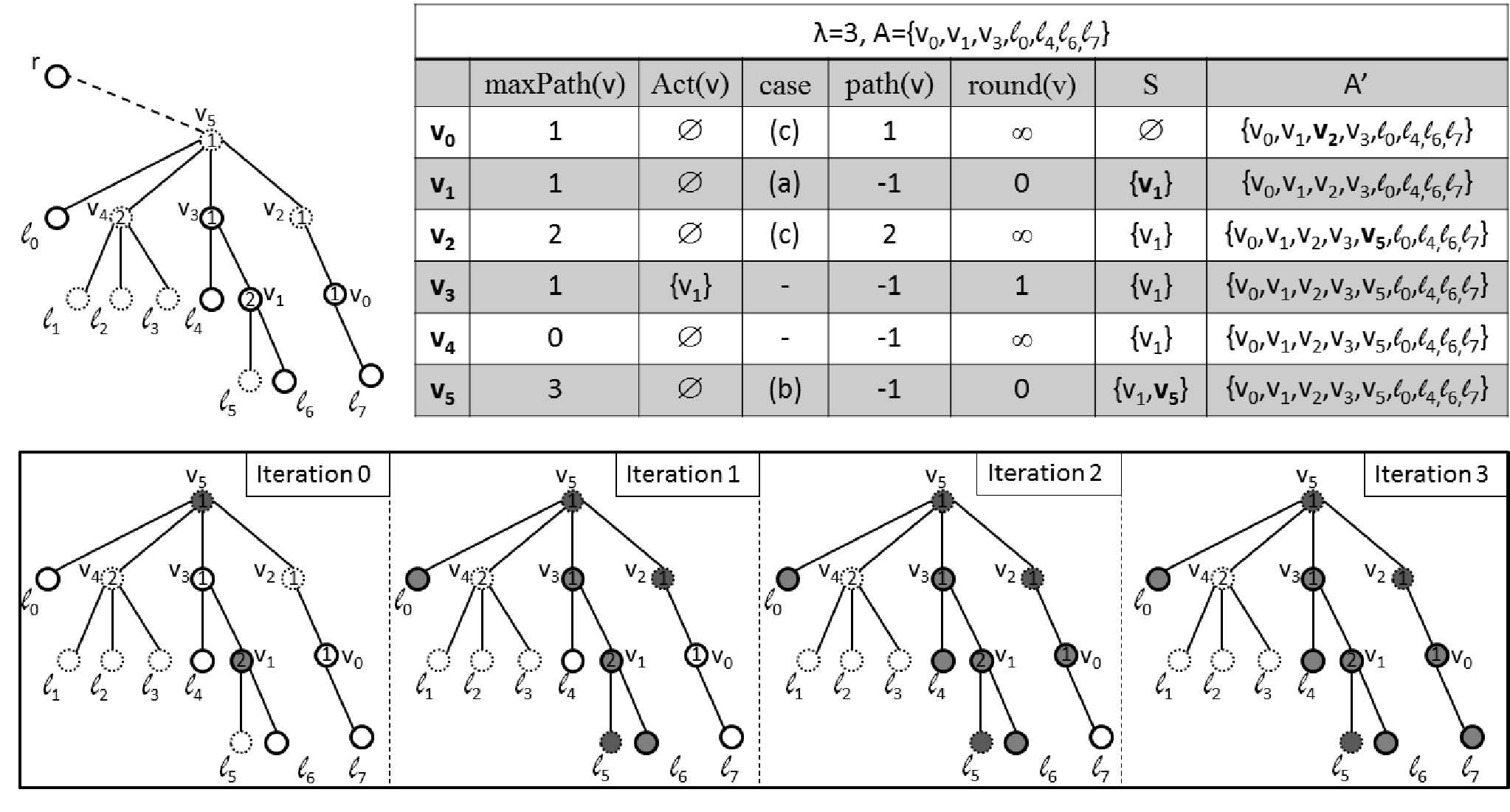
Algorithm 1 (λ,A)−(\lambda,A)-TSS on Trees
Input: A tree T=(V,E)T=(V,E), thresholds function t:V→ℕt:V\rightarrow\mathbb{N}, a latency bound λ∈ℕ\lambda\in\mathbb{N} and a set to be activated A⊆VA\subseteq V.
Output: S⊆VS\subseteq V of minimum size such that A⊆A​c​t​i​v​e​[S,λ].A\subseteq Active[S,\lambda].
1 S=∅;S=\emptyset;
2 A′=A;A^{\prime}=A;
3 Fix a root r∈Vr\in V // T⁡(r)T(r) denotes the tree TT rooted at rr
4 forall vv in the set of T⁡(r)T(r) leaves do
    5 r​o​u​n​d​(v)=∞round(v)=\infty
    6 if v∈A′v\in A^{\prime} then // vv belongs to the set of nodes to be activated
       7 A′=A′∪{p⁡(v)}A^{\prime}=A^{\prime}\cup\{p(v)\} // p⁡(v)p(v) denotes vv’s parent
       8 p​a​t​h​(v)=0path(v)=0
    9 else
       10 p​a​t​h​(v)=−1path(v)=-1
11 forall vv in the set of T⁡(r)T(r) internal nodes, listed in reverse order with respect to the time they are visited by a breadth-first traversal from rr do
    12 m​a​x​P​a​t​h​(v)=1+maxu∈C⁡(v)⁡p​a​t​h​(u)maxPath(v)=1+\max_{u\in C(v)}path(u) // C⁡(v)C(v) is the set of vv’children
    13 A​c​t​(v)={u∈C⁡(v)|r​o​u​n​d​(u)<λ−m​a​x​P​a​t​h​(v)}Act(v)=\{u\in C(v)\ |\ round(u)<\lambda-maxPath(v)\}
    14 p​a​t​h​(v)=−1path(v)=-1
    15 r​o​u​n​d​(v)=1+mint⁡(v)⁡{r​o​u​n​d​(u)|u∈C⁡(v)}round(v)=1+\min^{t(v)}\{round(u)\ |\ u\in C(v)\}
    16 if v∈A′v\in A^{\prime} then // vv has to be activated
       17 if v≠rv\neq r then
          18 switch do
             19 case (|A​c​t​(v)|≤t⁡(v)−2)(|Act(v)|{\leq}t(v){-}2) OR (m​a​x​P​a​t​h​(v)=λ)(maxPath(v)=\lambda) do
                20 S=S∪{v}S=S\cup\{v\} // vv has to be in the target set
                21 r​o​u​n​d​(v)=0round(v)=0
             22 case (|A​c​t​(v)|=t⁡(v)−1)(|Act(v)|=t(v){-}1) AND (m​a​x​P​a​t​h​(v)<λ)(maxPath(v)<\lambda) do
                23 A′=A′∪{p⁡(v)}A^{\prime}=A^{\prime}\cup\{p(v)\} // vv will be activated thanks to its parent p⁡(v)p(v)
                24 p​a​t​h​(v)=m​a​x​P​a​t​h​(v)path(v)=maxPath(v)
       25 else // vv is the root
          26 if (|A​c​t​(v)|≤t⁡(v)−1)(|Act(v)|\leq t(v){-}1) then
             27 S=S∪{v}S=S\cup\{v\}
             28 r​o​u​n​d​(v)=0round(v)=0
29 return (SS)

Refer to caption

Figure 1: An example of execution of the algorithm (λ,A)−(\lambda,A)-TSS on Tree: (left) a subtree rooted in v5v_{5} (subscripts describe the order in which nodes are analyzed by the algorithm), each node is depicted as a circle and its threshold is given inside the circle. Circles having a solid border represent nodes in the set AA; (right) the first 66 steps of the algorithm are shown in the table; (bottom) the activation process is shown. Activated nodes are shaded. At round 0, S={v1,v5}S=\{v_{1},v_{5}\}.

Time complexity. The initialization (line 1-10) requires time O⁡(|V|)O(|V|). The order in which nodes have to be considered is determined using a BFS which requires time O⁡(|V|)O(|V|) on a tree. The forall (line 11) considers all the internal nodes: the algorithm analyzes each internal node vv in time O⁡(|C⁡(v)|)O(|C(v)|). We notice that the computation in line 1515 can be executed in O⁡(|C⁡(v)|)O(|C(v)|) by using an algorithm that solve the selection problem in linear time (see for instance [9]). Overall the complexity of the algorithm is O⁡(|V|)+∑v∈VO⁡(|C⁡(v)|)=O⁡(|V|).O(|V|)+\sum_{v\in V}O(|C(v)|)=O(|V|).

Correctness. Consider the computed solution SS. Let 𝖠𝖼𝗍𝗂𝗏𝖾⁡[S,0]=S{\sf Active}[S,0]=S and 𝖠𝖼𝗍𝗂𝗏𝖾⁡[S,i]{\sf Active}[S,i] be the sets of nodes which become active within the ii–th round of the activation process.

Lemma 1.

Algorithm (λ,A)(\lambda,A)–TSS on Tree outputs a solution for the (λ,A)(\lambda,A)-Target Set Selection problem on T=(V,E)T=(V,E).

Proof.

Given a node v∈Vv\in V, let a⁡(v)=min⁡{λ−m​a​x​P​a​t​h​(v),r​o​u​n​d​(v)}a(v)=\min\{\lambda-maxPath(v),round(v)\}; for a leaf node we assume m​a​x​P​a​t​h​(v)=0maxPath(v)=0. We prove, by induction on a=0,1,…,a=0,1,\dots, that for each v∈A′v\in A^{\prime}, s.t. a⁡(v)=aa(v)=a we have

v∈𝖠𝖼𝗍𝗂𝗏𝖾⁡[S,a]v\in{\sf Active}[S,a] (3)

For a=0,a=0, let vv be a node such that a⁡(v)=0a(v)=0. This implies that r​o​u​n​d​(v)=0round(v)=0 or λ−m​a​x​P​a​t​h​(v)=0\lambda-maxPath(v)=0; therefore, v∈S=𝖠𝖼𝗍𝗂𝗏𝖾⁡[S,0]v\in S={\sf Active}[S,0].

Now fix a>0a>0 and assume that w∈𝖠𝖼𝗍𝗂𝗏𝖾⁡[S,a⁡(w)]w\in{\sf Active}[S,a(w)] for any node ww with a⁡(w)≤a−1a(w)\leq a-1. We will prove that v∈𝖠𝖼𝗍𝗂𝗏𝖾⁡[S,a⁡(v)]v\in{\sf Active}[S,a(v)] holds for any node vv with a⁡(v)=aa(v)=a.

Let vv be such that a⁡(v)=a.a(v)=a. When vv is processed, there are three possible cases:

  • •

    CASE vv is added to the target set SS.
    Actually, this case cannot occur under the standing hypothesis that a>0a>0 since, if v∈Sv\in S then v∈𝖠𝖼𝗍𝗂𝗏𝖾⁡[S,0]v\in{\sf Active}[S,0] which would imply a⁡(v)=0<aa(v)=0<a.

  • •

    CASE (|A​c​t​(v)|≥t⁡(v)CLOSE(|Act(v)|\geq t(v)).
    We know that for each u∈A​c​t​(v)u\in Act(v) it holds r​o​u​n​d​(u)<λ−m​a​x​P​a​t​h​(v)round(u)<\lambda-maxPath(v).
    In case a=λ−m​a​x​P​a​t​h​(v)a=\lambda-maxPath(v), we have a⁡(u)≤r​o​u​n​d​(u)≤λ−m​a​x​P​a​t​h​(v)−1=a−1.a(u)\leq round(u)\leq\lambda-maxPath(v)-1=a-1.
    Analogously, if a=r​o​u​n​d​(v)a=round(v). The algorithm poses r​o​u​n​d​(v)≥r​o​u​n​d​(u)+1round(v)\geq round(u)+1 for each u∈A​c​t​(v)u\in Act(v). Therefore, a⁡(u)≤r​o​u​n​d​(u)≤a−1a(u)\leq round(u)\leq a-1.
    In both the above cases the inductive hypothesis applies to each u∈A​c​t​(v)u\in Act(v), that is A​c​t​(v)⊆𝖠𝖼𝗍𝗂𝗏𝖾⁡[S,a−1]Act(v)\subseteq{\sf Active}[S,a-1]. Since |A​c​t​(v)|≥t⁡(v)|Act(v)|\geq t(v) we have v∈𝖠𝖼𝗍𝗂𝗏𝖾⁡[S,a]v\in{\sf Active}[S,a].

  • •

    CASE (|A​c​t​(v)|=t⁡(v)−1)(|Act(v)|=t(v){-}1), v≠rv\neq r.
    In such a case the algorithm sets r​o​u​n​d​(v)=1+mint⁡(v)⁡{r​o​u​n​d​(u)|u∈C⁡(v)}round(v)=1+\min^{t(v)}\{round(u)\ |\ u\in C(v)\} where mint⁡(v)⁡C\min^{t(v)}C denotes the t⁡(v)t(v)–th smallest element in the set CC. Since |A​c​t​(v)|=t⁡(v)−1|Act(v)|=t(v){-}1, we have that r​o​u​n​d​(v)>λ−m​a​x​P​a​t​h​(v)round(v)>\lambda-maxPath(v), hence a⁡(v)=λ−m​a​x​P​a​t​h​(v)a(v)=\lambda-maxPath(v).
    Recalling that for each u∈A​c​t​(v)u\in Act(v) it holds r​o​u​n​d​(u)<λ−m​a​x​P​a​t​h​(v)round(u)<\lambda-maxPath(v), as above we have that the inductive hypothesis applies to each u∈A​c​t​(v)u\in Act(v), that is A​c​t​(v)⊆𝖠𝖼𝗍𝗂𝗏𝖾⁡[S,a−1]Act(v)\subseteq{\sf Active}[S,a-1].
    Consider now the parent p⁡(v)p(v) of vv. The algorithm implies m​a​x​P​a​t​h​(p⁡(v))≥m​a​x​P​a​t​h​(v)+1maxPath(p(v))\geq maxPath(v)+1. Hence λ−m​a​x​P​a​t​h​(p⁡(v))≤λ−m​a​x​P​a​t​h​(v)−1=a−1\lambda-maxPath(p(v))\leq\lambda-maxPath(v)-1=a-1 and the inductive hypothesis applies also to p⁡(v)p(v). Therefore, {p⁡(v)}∪A​c​t​(v)\{p(v)\}\cup Act(v) is a subset of size t⁡(v)t(v) of 𝖠𝖼𝗍𝗂𝗏𝖾⁡[S,a−1]{\sf Active}[S,a-1] and v∈𝖠𝖼𝗍𝗂𝗏𝖾⁡[S,a]v\in{\sf Active}[S,a].

We finally notice that a⁡(v)=min⁡{λ−m​a​x​P​a​t​h​(v),r​o​u​n​d​(v)}≤λa(v)=\min\{\lambda-maxPath(v),round(v)\}\leq\lambda for each v∈A′v\in A^{\prime}. Indeed, the smallest possible value of p​a​t​h​()path() is −1-1, which implies that m​a​x​P​a​t​h​(v)≥0maxPath(v)\geq 0 for any vv. ∎

Let T⁡(r)=(V,E)T(r)=(V,E) be a tree rooted at a r∈Vr\in V, and let X⊆VX\subseteq V be a target set such that A​c​t​i​v​e​[X,λ]⊇AActive[X,\lambda]\supseteq A. Let T⁡(v)T(v) be the subtree of T⁡(r)T(r) rooted at a node vv. Henceforth let 𝖠𝖼𝗍𝗂𝗏𝖾⁡[X,i,T⁡(v)]{\sf Active}[X,i,T(v)] be the set of nodes that is active at round ii by targeting X∩T⁡(v)X\cap T(v) in the subtree T⁡(v)T(v). Notice that while XX is a target set for T⁡(r)T(r) this not necessarily means that X∩T⁡(v)X\cap T(v) is a target set for T⁡(v)T(v).

–

r​o​u​n​dX​(v)={i if v∈𝖠𝖼𝗍𝗂𝗏𝖾⁡[X,i,T⁡(v)]∖𝖠𝖼𝗍𝗂𝗏𝖾⁡[X,i−1,T⁡(v)]0 if v∈X∞ otherwiseround_{X}(v)=\begin{cases}i&\mbox{ if $v\in{\sf Active}[X,i,T(v)]\setminus{\sf Active}[X,i-1,T(v)]$}\\ 0&\mbox{ if $v\in X$}\\ \infty&\mbox{ otherwise}\end{cases}

–

p​a​t​hX​(v)={0 if v∈A is a leaf AND v∉Xi if (m​a​x​P​a​t​hX​(v)=i<λ) AND (|𝖠𝖼𝗍𝗂𝗏𝖾⁡[X,λ−i−1,T⁡(v)]∩C⁡(v)|=t⁡(v)−1)  AND (v∈ACLOSE OR OPENm​a​x​P​a​t​hX​(v)>0) AND (v∉X)path_{X}(v)=\begin{cases}0&\mbox{ if $v\in A$ is a leaf AND $v\notin X$}\\ i&\mbox{ if $(maxPath_{X}(v)=i<\lambda)$}\\ &\mbox{ $\quad$ AND $(|{\sf Active}[X,\lambda-i-1,T(v)]\cap C(v)|=t(v)-1)$ }\\ &\mbox{ $\quad$ AND $(v\in A$ OR $maxPath_{X}(v)>0)$}\mbox{ AND $(v\notin X)$}\\ \end{cases}

–

m​a​x​P​a​t​hX​(v)={1+maxu∈C⁡(v)⁡p​a​t​hX​(u) if v is an internal node (C⁡(v)≠∅)0 if v is a leaf.maxPath_{X}(v)=\begin{cases}1+\max_{u\in C(v)}path_{X}(u)&\mbox{ if $v$ is an internal node ($C(v)\neq\emptyset$)}\\ 0&\mbox{ if $v$ is a leaf.}\end{cases}

When X=SX=S then the values r​o​u​n​d​(v)round(v) and p​a​t​h​(v)path(v), computed by the algorithm, correspond to the values defined above.

Lemma 2.

If X=SX=S then for each node v∈V,v\in V, r​o​u​n​d​(v)=r​o​u​n​dS​(v)round(v)=round_{S}(v), p​a​t​h​(v)=p​a​t​hS​(v)path(v)=path_{S}(v) and A​c​t​(v)=𝖠𝖼𝗍𝗂𝗏𝖾⁡[S,λ−m​a​x​P​a​t​hS​(v)−1,T⁡(v)]∩C⁡(v)Act(v)={\sf Active}[S,\lambda-maxPath_{S}(v)-1,T(v)]\cap C(v).

Proof.

First we show by induction on the height of vv that r​o​u​n​d​(v)=r​o​u​n​dS​(v)round(v)=round_{S}(v).

Induction Basis: For each leaf vv we have T⁡(v)=vT(v)=v. Since v∉Sv\notin S, we have that v∉𝖠𝖼𝗍𝗂𝗏𝖾⁡[S,j,v]v\notin{\sf Active}[S,j,v] for any value of jj. Hence r​o​u​n​dS​(v)=r​o​u​n​d​(v)=∞round_{S}(v)=round(v)=\infty (line 5).

Induction step: Let vv an internal node and suppose that the claim is true for any children of vv.
If v∈Sv\in S the claim is trivially true, r​o​u​n​dS​(v)=0=r​o​u​n​d​(v)round_{S}(v)=0=round(v) (lines 21 and 28).
Otherwise, let r​o​u​n​d​(v)=i=1+mint⁡(v)⁡{r​o​u​n​d​(u)|u∈C⁡(v)}round(v)=i=1+\min^{t(v)}\{round(u)\ |\ u\in C(v)\} where mint⁡(v)⁡C\min^{t(v)}C denotes the t⁡(v)t(v)–th smallest element in the set CC. By induction i=1+mint⁡(v)⁡{r​o​u​n​dS​(u)|u∈C⁡(v)}i=1+\min^{t(v)}\{round_{S}(u)\ |\ u\in C(v)\}. There is a set CS​(v)⊆C​(v)C_{S}(v)\subseteq C(v) such that |CS​(v)|=t​(v)|C_{S}(v)|=t(v), ∀w∈CS​(v),r​o​u​n​dS​(w)≤i−1\forall w\in C_{S}(v),round_{S}(w)\leq i-1 and ∃u∈CS​(v)\exists u\in C_{S}(v) such that r​o​u​n​dS​(u)=i−1round_{S}(u)=i-1. Hence, ∀w∈CS​(v),w∈𝖠𝖼𝗍𝗂𝗏𝖾⁡[S,i−1,T⁡(w)]\forall w\in C_{S}(v),w\in{\sf Active}[S,i-1,T(w)] and ∃u∈CS​(v)\exists u\in C_{S}(v) such that u∈𝖠𝖼𝗍𝗂𝗏𝖾⁡[S,i−1,T⁡(u)]∖𝖠𝖼𝗍𝗂𝗏𝖾⁡[S,i−2,T⁡(u)]u\in{\sf Active}[S,i-1,T(u)]\setminus{\sf Active}[S,i-2,T(u)] and we have v∈𝖠𝖼𝗍𝗂𝗏𝖾⁡[S,i,T⁡(v)]∖𝖠𝖼𝗍𝗂𝗏𝖾⁡[S,i−1,T⁡(v)]v\in{\sf Active}[S,i,T(v)]\setminus{\sf Active}[S,i-1,T(v)] which means that r​o​u​n​dS​(v)=iround_{S}(v)=i.

Now we show that p​a​t​h​(v)=p​a​t​hS​(v)path(v)=path_{S}(v) and A​c​t​(v)=𝖠𝖼𝗍𝗂𝗏𝖾⁡[S,λ−m​a​x​P​a​t​hS​(v)−1,T⁡(v)]∩C⁡(v)Act(v)={\sf Active}[S,\lambda-maxPath_{S}(v)-1,T(v)]\cap C(v). Again, we argue by induction on the height of vv.

Induction Basis. For each leaf vv, if v∈Av\in A then p​a​t​hS​(v)=p​a​t​h​(v)=0path_{S}(v)=path(v)=0 (line 8). On the other hand if v∉Av\notin A then p​a​t​h​(v)=−1path(v)=-1 (line 10). Moreover, since v∉Av\notin A and has no children p​a​t​hS​(v)≠ipath_{S}(v)\neq i. Hence p​a​t​hS​(v)=−1.path_{S}(v)=-1.
Moreover since C⁡(v)=∅C(v)=\emptyset we have A​c​t​(v)=𝖠𝖼𝗍𝗂𝗏𝖾⁡[S,λ−m​a​x​P​a​t​hS​(v)−1,T⁡(v)]∩C⁡(v)=∅.Act(v)={\sf Active}[S,\lambda-maxPath_{S}(v)-1,T(v)]\cap C(v)=\emptyset.

Induction Step. Let v≠rv\neq r be an internal node and suppose that the claim is true for any children of vv. Hence, ∀u∈C⁡(v),\forall u\in C(v), p​a​t​h​(u)=p​a​t​hS​(u)path(u)=path_{S}(u) and we have m​a​x​P​a​t​hS​(v)=1+maxu∈C⁡(v)⁡p​a​t​h​(u)=m​a​x​P​a​t​h​(v).maxPath_{S}(v)=1+\max_{u\in C(v)}path(u)=maxPath(v). Notice that m​a​x​P​a​t​h​(v)=1+maxu∈C⁡(v)⁡p​a​t​hS​(u)≥0maxPath(v)=1+\max_{u\in C(v)}path_{S}(u)\geq 0.

We are going to show that A​c​t​(v)=𝖠𝖼𝗍𝗂𝗏𝖾⁡[S,λ−m​a​x​P​a​t​hS​(v)−1,T⁡(v)]∩C⁡(v)Act(v)={\sf Active}[S,\lambda-maxPath_{S}(v)-1,T(v)]\cap C(v).

Let u∈A​c​t​(v)u\in Act(v). Hence u∈C⁡(v)u\in C(v) and r​o​u​n​d​(u)<λ−m​a​x​P​a​t​h​(v)round(u)<\lambda-maxPath(v). Since r​o​u​n​d​(u)=r​o​u​n​dS​(u)round(u)=round_{S}(u) and by induction m​a​x​P​a​t​h​(v)=m​a​x​P​a​t​hS​(v)maxPath(v)=maxPath_{S}(v) we have r​o​u​n​dS​(u)≤λ−m​a​x​P​a​t​h​(v)−1round_{S}(u)\leq\lambda-maxPath(v)-1. Hence u∈𝖠𝖼𝗍𝗂𝗏𝖾⁡[S,λ−m​a​x​P​a​t​h​(v)−1,T⁡(u)]u\in{\sf Active}[S,\lambda-maxPath(v)-1,T(u)] and therefore u∈𝖠𝖼𝗍𝗂𝗏𝖾⁡[S,λ−m​a​x​P​a​t​h​(v)−1,T⁡(v)]∩C⁡(v)u\in{\sf Active}[S,\lambda-maxPath(v)-1,T(v)]\cap C(v). Hence A​c​t​(v)⊆𝖠𝖼𝗍𝗂𝗏𝖾⁡[S,λ−m​a​x​P​a​t​h​(v)−1,T⁡(v)]∩C⁡(v)Act(v)\subseteq{\sf Active}[S,\lambda-maxPath(v)-1,T(v)]\cap C(v).

Let u∈𝖠𝖼𝗍𝗂𝗏𝖾⁡[S,λ−m​a​x​P​a​t​h​(v)−1,T⁡(v)]∩C⁡(v)u\in{\sf Active}[S,\lambda-maxPath(v)-1,T(v)]\cap C(v). Hence u∈C⁡(v)u\in C(v) and r​o​u​n​dS​(u)≤λ−m​a​x​P​a​t​h​(v)−1round_{S}(u)\leq\lambda-maxPath(v)-1. Since r​o​u​n​d​(u)=r​o​u​n​dS​(u)round(u)=round_{S}(u) and by induction m​a​x​P​a​t​h​(v)=m​a​x​P​a​t​hS​(v)maxPath(v)=maxPath_{S}(v) we have r​o​u​n​d​(u)<λ−m​a​x​P​a​t​h​(v)round(u)<\lambda-maxPath(v) and therefore u∈A​c​t​(v)u\in Act(v). Hence A​c​t​(v)⊇𝖠𝖼𝗍𝗂𝗏𝖾⁡[S,λ−m​a​x​P​a​t​h​(v)−1,T⁡(v)]∩C⁡(v)Act(v)\supseteq{\sf Active}[S,\lambda-maxPath(v)-1,T(v)]\cap C(v).

Since vv is an internal node, in order to show that p​a​t​h​(v)=p​a​t​hS​(v)path(v)=path_{S}(v) two cases have to be considered: p​a​t​hS​(u)=m​a​x​P​a​t​h​(v)path_{S}(u)=maxPath(v) or p​a​t​hS​(u)=−1path_{S}(u)=-1.

case (p​a​t​h​(v)=m​a​x​P​a​t​h​(v)path(v)=maxPath(v)):

According to the algorithm this case happens when

(a)

v∈A′v\in A^{\prime} AND

(b)

m​a​x​P​a​t​h​(v)<λmaxPath(v)<\lambda AND

(c)

|A​c​t​(v)|=t⁡(v)−1|Act(v)|=t(v)-1

Moreover, when this case occur vv is not added to SS (i.e., v∉Sv\notin S). Thanks to (a) we have that v∈A′v\in A^{\prime} if either v∈Av\in A (line 2) or vv has a children uu such that p​a​t​h​(u)=m​a​x​P​a​t​h​(u)≥0path(u)=maxPath(u)\geq 0 (line 23-24) or vv has a children uu such that u∈Au\in A and uu is a leaf, that is p​a​t​h​(u)=0path(u)=0 (line 7-8). Hence we have v∈A′v\in A^{\prime} iff v∈Av\in A OR m​a​x​P​a​t​hS​(v)>0.maxPath_{S}(v)>0.

Thanks to (b) and (c) we have that m​a​x​P​a​t​hS​(v)<λmaxPath_{S}(v)<\lambda and |𝖠𝖼𝗍𝗂𝗏𝖾⁡[S,λ−m​a​x​P​a​t​h​(v)−1,T⁡(v)]∩C⁡(v)|=t⁡(v)−1.|{\sf Active}[S,\lambda-maxPath(v)-1,T(v)]\cap C(v)|=t(v)-1. Hence using (a), (b) and (c) and the fact that v∉Sv\notin S we have p​a​t​hS​(v)=m​a​x​P​a​t​h​(v)path_{S}(v)=maxPath(v).

case (p​a​t​h​(v)=−1path(v)=-1):

In this case one of the above requirement is not satisfied and we have p​a​t​hS​(v)=−1path_{S}(v)=-1.

Similar reasoning can be used to show that p​a​t​h​(r)=p​a​t​hS​(r)path(r)=path_{S}(r) and A​c​t​(r)=𝖠𝖼𝗍𝗂𝗏𝖾⁡[S,λ−m​a​x​P​a​t​hS​(r)−1,T⁡(r)]∩C⁡(r)Act(r)={\sf Active}[S,\lambda-maxPath_{S}(r)-1,T(r)]\cap C(r). ∎

Let XX be a target set solution (i.e., 𝖠𝖼𝗍𝗂𝗏𝖾⁡[X,λ]⊇A{\sf Active}[X,\lambda]\supseteq A). For an edge (v,u)(v,u) we say that vv activates uu and write v→uv\to u if v∈𝖠𝖼𝗍𝗂𝗏𝖾⁡[X,i−1]v\in{\sf Active}[X,i-1] and u∈𝖠𝖼𝗍𝗂𝗏𝖾⁡[X,i]∖𝖠𝖼𝗍𝗂𝗏𝖾⁡[X,i−1]u\in{\sf Active}[X,i]\setminus{\sf Active}[X,i-1], for some 1≤i≤λ1\leq i\leq\lambda. An activation path v↝uv\leadsto u from vv to uu is a path in TT such that v=x0→x1→…→xk=uv=x_{0}\to x_{1}\to\ldots\to x_{k}=u with xj∈𝖠𝖼𝗍𝗂𝗏𝖾⁡[X,ij]∖𝖠𝖼𝗍𝗂𝗏𝖾⁡[X,ij−1]x_{j}\in{\sf Active}[X,i_{j}]\setminus{\sf Active}[X,i_{j}-1] for 0≤i1<i2<…<ik≤λ.0\leq i_{1}<i_{2}<\ldots<i_{k}\leq\lambda. In other words xix_{i} is activated before xi+1x_{i+1}, for i=0,…,k−1i=0,\ldots,k-1.

Lemma 3.

Let XX be a target set solutions (i.e., 𝖠𝖼𝗍𝗂𝗏𝖾⁡[X,λ]⊇A{\sf Active}[X,\lambda]\supseteq A) and v∈Vv\in V. If m​a​x​P​a​t​hX​(v)=imaxPath_{X}(v)=i then there is an activation path of length ii in T⁡(v)T(v) starting at vv and ending at a node u∈Au\in A.

Proof.

Since m​a​x​P​a​t​hX​(v)=imaxPath_{X}(v)=i then there is a path in T⁡(v)T(v) from vv to a node uu such that v=xi→xi−1→…→x0=uv=x_{i}\to x_{i-1}\to\ldots\to x_{0}=u where for each i=0,1,…,i−1,i=0,1,\ldots,i-1, p​a​t​hX​(xi)=i.path_{X}(x_{i})=i. We are able to show by induction that for each j=0,1,…,i−1,j=0,1,\ldots,i-1, xjx_{j} is activated after xj+1x_{j+1}.

Induction basis: j=0j=0. Hence, p​a​t​hX​(x0)=0path_{X}(x_{0})=0 which means that x0∉Xx_{0}\notin X. There are two case to consider:

(x0x_{0} is a leaf)

hence x0∈Ax_{0}\in A. Moreover since x0x_{0} has no children we have that x0x_{0} will be activated after its parent x1x_{1}.

(x0x_{0} is an internal node)

since p​a​t​hX​(x0)=0path_{X}(x_{0})=0 we have that m​a​x​P​a​t​hX​(x0)=0maxPath_{X}(x_{0})=0 hence x0∈Ax_{0}\in A. Moreover, since |𝖠𝖼𝗍𝗂𝗏𝖾⁡[X,λ−1,T⁡(x0)]∩C⁡(x0)|=t⁡(x0)−1|{\sf Active}[X,\lambda-1,T(x_{0})]\cap C(x_{0})|=t(x_{0})-1 we have that x0x_{0} will be activated after its parent x1x_{1}. Otherwise x0x_{0} will not be activated by round λ−1\lambda-1.

Induction step: j=ij=i. Hence, p​a​t​hX​(xj)=m​a​x​P​a​t​hX​(xj)=jpath_{X}(x_{j})=maxPath_{X}(x_{j})=j which means that xi∉Xx_{i}\notin X. Moreover, by induction, we know that ∀j<i\forall j<i, xjx_{j} is activated after xj+1x_{j+1}. Hence in order to activate x0x_{0} by round λ\lambda, xjx_{j} has to be activated by round λ−j−1\lambda-j-1. Since |𝖠𝖼𝗍𝗂𝗏𝖾⁡[X,λ−j−1,T⁡(xj)]∩C⁡(xj)|=t⁡(xj)−1|{\sf Active}[X,\lambda-j-1,T(x_{j})]\cap C(x_{j})|=t(x_{j})-1 we have that xjx_{j} will be activated after its parent xj+1x_{j+1}. Otherwise xjx_{j} will not be activated by round λ−j−1\lambda-j-1. ∎

Let XX and YY be two target set solutions and v∈Vv\in V. The following properties hold:

Property 1.

If r​o​u​n​dX​(v)>r​o​u​n​dY​(v)round_{X}(v)>round_{Y}(v) and v∉Yv\notin Y then there exists u∈C⁡(v)u\in C(v) such that r​o​u​n​dX​(u)>r​o​u​n​dY​(u)round_{X}(u)>round_{Y}(u).

Proof.

Let r​o​u​n​dY​(v)=iround_{Y}(v)=i we have that v∈𝖠𝖼𝗍𝗂𝗏𝖾⁡[Y,i,T⁡(v)]∖𝖠𝖼𝗍𝗂𝗏𝖾⁡[Y,i−1,T⁡(v)]v\in{\sf Active}[Y,i,T(v)]\setminus{\sf Active}[Y,i-1,T(v)]. Hence, there is a set CY⊆C⁡(v)C_{Y}\subseteq C(v) such that |CY|=t⁡(v)|C_{Y}|=t(v) and ∀u∈CY,u∈𝖠𝖼𝗍𝗂𝗏𝖾⁡[Y,i−1,T⁡(u)]\forall u\in C_{Y},u\in{\sf Active}[Y,i-1,T(u)] (i.e., ∀u∈CY,r​o​u​n​dY​(u)≤i−1\forall u\in C_{Y},round_{Y}(u)\leq i-1). On the other hand, since r​o​u​n​dX​(v)>iround_{X}(v)>i the size of the set CX={u∈C⁡(v)|r​o​u​n​dX​(u)≤i−1}C_{X}=\{u\in C(v)|round_{X}(u)\leq i-1\} is at most t⁡(v)−1t(v)-1. Hence there is at least a vertex u∈C⁡(v)u\in C(v) such that r​o​u​n​dX​(u)>r​o​u​n​dY​(u)round_{X}(u)>round_{Y}(u). ∎

Property 2.

If v∉Xv\notin X then m​a​x​P​a​t​hX​(v)<λmaxPath_{X}(v)<\lambda AND |𝖠𝖼𝗍𝗂𝗏𝖾⁡[X,λ−m​a​x​P​a​t​hX​(v)−1,T⁡(v)]∩C⁡(v)|>t⁡(v)−2|{\sf Active}[X,\lambda-maxPath_{X}(v)-1,T(v)]\cap C(v)|>t(v)-2.

Proof.

In the following we show that if either m​a​x​P​a​t​hX​(v)≥λmaxPath_{X}(v)\geq\lambda or |𝖠𝖼𝗍𝗂𝗏𝖾⁡[X,λ−m​a​x​P​a​t​hX​(v)−1,T⁡(v)]∩C⁡(v)|≤t⁡(v)−2|{\sf Active}[X,\lambda-maxPath_{X}(v)-1,T(v)]\cap C(v)|\leq t(v)-2 then v∈X.v\in X.

When m​a​x​P​a​t​hX​(v)≥λmaxPath_{X}(v)\geq\lambda then by Lemma 3 there is an activation path of length at least λ\lambda in T⁡(v)T(v) starting at vv and ending at a node u∈Au\in A and we have that vv has to be active at round 00.

When |𝖠𝖼𝗍𝗂𝗏𝖾⁡[X,λ−m​a​x​P​a​t​hX​(v)−1,T⁡(v)]∩C⁡(v)|≤t⁡(v)−2|{\sf Active}[X,\lambda-maxPath_{X}(v)-1,T(v)]\cap C(v)|\leq t(v)-2, since by Lemma 3 there is an activation path of length m​a​x​P​a​t​hX​(v)maxPath_{X}(v) starting at vv and ending at a node u∈Au\in A, we have that vv has to be active at round λ−m​a​x​P​a​t​hX​(v)\lambda-maxPath_{X}(v) (i.e., vv should belong to 𝖠𝖼𝗍𝗂𝗏𝖾⁡[X,λ−m​a​x​P​a​t​hX​(v)]{\sf Active}[X,\lambda-maxPath_{X}(v)]). Since |𝖠𝖼𝗍𝗂𝗏𝖾⁡[X,λ−m​a​x​P​a​t​hX​(v)−1,T⁡(v)]∩C⁡(v)|≤t⁡(v)−2|{\sf Active}[X,\lambda-maxPath_{X}(v)-1,T(v)]\cap C(v)|\leq t(v)-2 then vv will not be activated (even considering its parent) at round λ−m​a​x​P​a​t​hX​(v)\lambda-maxPath_{X}(v). Hence vv has to be in XX. ∎

Lemma 4.

Algorithm (λ,A)−(\lambda,A)-TSS on Tree outputs an optimal solution for the (λ,A)−(\lambda,A)- Target Set Selection problem on T=(V,E)T=(V,E).

Proof.

Let SS and OO be respectively the solutions found by the Algorithm (λ,A)−(\lambda,A)-TSS on Tree and an optimal solution. For each v∈Vv\in V let S⁡(v)=S∩T⁡(v)S(v)=S\cap T(v) (resp. O⁡(v)=O∩T⁡(v)O(v)=O\cap T(v)) be the set of target nodes in SS (resp. OO) which belong to T⁡(v)T(v). Let s⁡(u)=|S⁡(u)|s(u)=|S(u)| and o⁡(u)=|O⁡(u)|o(u)=|O(u)| be the cardinality of such sets. We will use the following claim.

Claim 1.

For any vertex v∈Vv\in V, if p​a​t​hS​(v)>p​a​t​hO​(v)path_{S}(v)>path_{O}(v) OR r​o​u​n​dS​(v)>r​o​u​n​dO​(v)round_{S}(v)>round_{O}(v) then s⁡(v)<o⁡(v).s(v)<o(v).

Proof.

We argue by induction on the height of v.v. The claims trivially hold when vv is a leaf. Since our algorithm does not target any leaf (i.e. v∉Sv\notin S), two cases need to be analyzed:

case (v∈Ov\in O):

then s⁡(v)=0<1=o⁡(v)s(v)=0<1=o(v) and the inequality is satisfied.

case (v∉Ov\notin O):

then r​o​u​n​dS​(v)=r​o​u​n​dO​(v)=∞round_{S}(v)=round_{O}(v)=\infty and p​a​t​hS​(v)=p​a​t​hO​(v)=0​ or −1path_{S}(v)=path_{O}(v)=0\mbox{ or }{-}1 depending whether v∈Av\in A or not. Hence none of the two conditions of the if are satisfied then the claim holds.

Now consider any internal vertex v∈Vv\in V. By induction, we have that ∀u∈C⁡(v),s⁡(u)≤o⁡(u)\forall u\in C(v),s(u)\leq o(u), hence

∑u∈C⁡(v)s⁡(u)≤∑u∈C⁡(v)o⁡(u).\sum_{u\in C(v)}s(u)\leq\sum_{u\in C(v)}o(u). (4)

There are four cases to consider:

case (v∉Sv\notin S and v∈Ov\in O):

Using eq. (4) we have s⁡(v)≤o⁡(v)−1<o⁡(v),s(v)\leq o(v)-1<o(v), hence the claim holds.

case (v∈Sv\in S and v∈Ov\in O):

We have p​a​t​hS​(v)=p​a​t​hO​(v)=−1path_{S}(v)=path_{O}(v)=-1 and r​o​u​n​dS​(v)=r​o​u​n​dO​(v)=0round_{S}(v)=round_{O}(v)=0. Hence none of the two conditions of the if statement are satisfied and the claim holds.

case (v∉Sv\notin S and v∉Ov\notin O):

if p​a​t​hS​(v)>p​a​t​hO​(v)path_{S}(v)>path_{O}(v) OR r​o​u​n​dS​(v)>r​o​u​n​dO​(v)round_{S}(v)>round_{O}(v) then in order to prove the claim we need to find a child uu of vv such that s⁡(u)<o⁡(u)s(u)<o(u).

In the following we analyze the two cases separately:

if r​o​u​n​dS​(v)>r​o​u​n​dO​(v)round_{S}(v)>round_{O}(v) then using Property 1 we have that there is a vertex u∈C⁡(v)u\in C(v) such that r​o​u​n​dS​(u)>r​o​u​n​dO​(u)round_{S}(u)>round_{O}(u). By induction on the height of vv we have that s⁡(u)<o⁡(u)s(u)<o(u).

if p​a​t​hS​(v)>p​a​t​hO​(v)path_{S}(v)>path_{O}(v) then p​a​t​hS​(v)≠−1path_{S}(v)\neq-1, hence by definition of p​a​t​hX​(⋅)path_{X}(\cdot),

m​a​x​P​a​t​hS​(v)=i<λ\displaystyle maxPath_{S}(v)=i<\lambda (5)
AND |𝖠𝖼𝗍𝗂𝗏𝖾⁡[S,λ−i−1,T⁡(v)]∩C⁡(v)|=t⁡(v)−1\displaystyle\mbox{ AND }|{\sf Active}[S,\lambda-i-1,T(v)]\cap C(v)|=t(v)-1 (6)
AND ​(v∈A​ OR ​m​a​x​P​a​t​hS​(v)>0)\displaystyle\mbox{ AND }(v\in A\mbox{ OR }maxPath_{S}(v)>0) (7)

There are two cases to consider:

case (p​a​t​hO​(v)≥0path_{O}(v)\geq 0):

then p​a​t​hO​(v)=m​a​x​P​a​t​hO​(v)<m​a​x​P​a​t​hS​(v)path_{O}(v)=maxPath_{O}(v)<maxPath_{S}(v) and there is a child uu of vv such that p​a​t​hS​(u)=m​a​x​P​a​t​hS​(v)−1>m​a​x​P​a​t​hO​(v)−1≥p​a​t​hO​(u)path_{S}(u)=maxPath_{S}(v)-1>maxPath_{O}(v)-1\geq path_{O}(u) and we have found the desired vertex because by induction we have s⁡(u)<o⁡(u)s(u)<o(u).

case (p​a​t​hO​(v)=−1path_{O}(v)=-1):

Since v∉Ov\notin O and by Property 2 we know that m​a​x​P​a​t​hO​(v)<λmaxPath_{O}(v)<\lambda AND |𝖠𝖼𝗍𝗂𝗏𝖾⁡[O,λ−m​a​x​P​a​t​hO​(v)−1,T⁡(v)]∩C⁡(v)|>t⁡(v)−2|{\sf Active}[O,\lambda-maxPath_{O}(v)-1,T(v)]\cap C(v)|>t(v)-2. Hence p​a​t​hO​(v)=−1path_{O}(v)=-1 can happen only for two reasons:

case (v∉Av\notin A and m​a​x​P​a​t​hO​(v)=0maxPath_{O}(v)=0):

Since v∉Av\notin A, then by eq. 7, there is a children uu of vv such that p​a​t​hS​(u)≥0>−1=p​a​t​hO​(u)path_{S}(u)\geq 0>-1=path_{O}(u) and we have found the desired vertex because by induction it holds that s⁡(u)<o⁡(u)s(u)<o(u).

case

(|𝖠𝖼𝗍𝗂𝗏𝖾⁡[O,λ−m​a​x​P​a​t​hO​(v)−1,T⁡(v)]∩C⁡(v)|≥t⁡(v)|{\sf Active}[O,\lambda-maxPath_{O}(v)-1,T(v)]\cap C(v)|\geq t(v)): Hence by equation 6 we have

|𝖠𝖼𝗍𝗂𝗏𝖾⁡[O,λ−j−1,T⁡(v)]∩C⁡(v)|>|𝖠𝖼𝗍𝗂𝗏𝖾⁡[S,λ−i−1,T⁡(v)]∩C⁡(v)||{\sf Active}[O,\lambda-j-1,T(v)]\cap C(v)|>|{\sf Active}[S,\lambda-i-1,T(v)]\cap C(v)|

where i=m​a​x​P​a​t​hS​(v)i=maxPath_{S}(v) and j=m​a​x​P​a​t​hO​(v)j=maxPath_{O}(v). If i=m​a​x​P​a​t​hS​(v)>m​a​x​P​a​t​hO​(v)=ji=maxPath_{S}(v)>maxPath_{O}(v)=j (i.e., 1+maxu∈C⁡(v)⁡p​a​t​hS​(u)>1+maxu∈C⁡(v)⁡p​a​t​hO​(u)1+\max_{u\in C(v)}path_{S}(u)>1+\max_{u\in C(v)}path_{O}(u)) then there is a child uu of vv such that p​a​t​hS​(u)>p​a​t​hO​(u)path_{S}(u)>path_{O}(u) and we have found the desired vertex because by induction we have s⁡(u)<o⁡(u)s(u)<o(u). On the other hand if i=m​a​x​P​a​t​hS​(v)≤m​a​x​P​a​t​hO​(v)=ji=maxPath_{S}(v)\leq maxPath_{O}(v)=j, then there exists a child u∈C⁡(v)u\in C(v) such that, u∈𝖠𝖼𝗍𝗂𝗏𝖾⁡[O,λ−j−1,T⁡(u)]∖𝖠𝖼𝗍𝗂𝗏𝖾⁡[O,λ−j−2,T⁡(u)]u\in{\sf Active}[O,\lambda-j-1,T(u)]\setminus{\sf Active}[O,\lambda-j-2,T(u)] and u∉𝖠𝖼𝗍𝗂𝗏𝖾⁡[S,λ−i−1,T⁡(u)]u\notin{\sf Active}[S,\lambda-i-1,T(u)]. Hence r​o​u​n​dO​(u)=λ−j−1≤λ−i−1<r​o​u​n​dS​(u)round_{O}(u)=\lambda-j-1\leq\lambda-i-1<round_{S}(u). By induction we have that s⁡(u)<o⁡(u)s(u)<o(u).

In all the cases above we are able to find the desired vertex and the claim holds.

case (v∈Sv\in S and v∉Ov\notin O):

Using eq. (4) we have s⁡(v)−1≤o⁡(v).s(v)-1\leq o(v). For each u∈C⁡(v)u\in C(v) we know by induction that s⁡(u)≤o⁡(u)s(u)\leq o(u). Since v∈Sv\in S we have p​a​t​hS​(v)=−1path_{S}(v)=-1 and r​o​u​n​dS​(v)=0round_{S}(v)=0, hence none of the two requirement of the if is satisfied hence the claim holds true.

∎

We show by induction on the height of the node that s⁡(v)≤o⁡(v)s(v)\leq o(v), for each v∈Vv\in V.
The inequality trivially holds when vv is a leaf. Since our algorithm does not target any leaf (i.e. v∉Sv\notin S), we have s⁡(v)=0s(v)=0. Since we have o⁡(v)=0o(v)=0 or o⁡(v)=1o(v)=1 according to whether vv belongs to the optimal solution, the inequality is always satisfied.
Now consider any internal node vv. By induction, s⁡(u)≤o⁡(u)s(u)\leq o(u) for each u∈C⁡(v)u\in C(v); hence

∑u∈C⁡(v)s⁡(u)≤∑u∈C⁡(v)o⁡(u).\sum_{u\in C(v)}s(u)\leq\sum_{u\in C(v)}o(u). (8)

It is not hard to see that if v∈Ov\in O by (8) we immediately have s⁡(v)≤o⁡(v).s(v)\leq o(v). The same result follows from (8) for the case where vv is neither in OO nor in S.S.
We are left with the case v∈Sv\in S and v∉Ov\not\in O In this case eq. (8) only gives s⁡(v)−1≤o⁡(v).s(v)-1\leq o(v). In order to obtain the desired result we need to find a child uu of vv such that s⁡(u)<o⁡(u)s(u)<o(u). We distinguish the following two cases:
case (v∉Av\notin A and m​a​x​P​a​t​hO​(v)=0maxPath_{O}(v)=0): Since v∈Sv\in S we have v∈A′v\in A^{\prime} (that is v∈Av\in A or m​a​x​P​a​t​hS​(v)>0maxPath_{S}(v)>0). Since v∈A′∖Av\in A^{\prime}\setminus A then m​a​x​P​a​t​hS​(v)>0maxPath_{S}(v)>0 and there is a children uu of vv such that p​a​t​hS​(u)≥0>−1=p​a​t​hO​(u)=−1path_{S}(u)\geq 0>-1=path_{O}(u)=-1 and we have found the desired vertex because by the Claim above we have s⁡(u)<o⁡(u)s(u)<o(u).
case (v∈Av\in A or m​a​x​P​a​t​hO​(v)>0maxPath_{O}(v)>0): Since v∈Sv\in S we have that either m​a​x​P​a​t​hS​(v)=λmaxPath_{S}(v)=\lambda or |A​c​t​(v)|=|𝖠𝖼𝗍𝗂𝗏𝖾⁡[S,λ−i−1,T⁡(v)]∩C⁡(v)|≤t⁡(v)−2|Act(v)|=|{\sf Active}[S,\lambda-i-1,T(v)]\cap C(v)|\leq t(v)-2 where i=m​a​x​P​a​t​hS​(v)i=maxPath_{S}(v). We consider the two subcases separately:

–

(m​a​x​P​a​t​hS​(v)=λmaxPath_{S}(v)=\lambda): Since v∉Ov\notin O, by Property 2, we have that m​a​x​P​a​t​hO​(v)<λmaxPath_{O}(v)<\lambda. Hence, there is a vertex u∈C⁡(v)u\in C(v) such that p​a​t​hS​(u)=λ−1>p​a​t​hO​(u)path_{S}(u)=\lambda-1>path_{O}(u) and we have found the desired vertex because, by the Claim we have o⁡(u)>s⁡(u)o(u)>s(u).

–

(|A​c​t​(v)|=|𝖠𝖼𝗍𝗂𝗏𝖾⁡[S,λ−m​a​x​P​a​t​hS​(v)−1,T⁡(v)]∩C⁡(v)|≤t⁡(v)−2|Act(v)|=|{\sf Active}[S,\lambda-maxPath_{S}(v)-1,T(v)]\cap C(v)|\leq t(v)-2): Since v∉Ov\notin O by Property 2 we have that |𝖠𝖼𝗍𝗂𝗏𝖾⁡[O,λ−m​a​x​P​a​t​hO​(v)−1,T⁡(v)]∩C⁡(v)|>t⁡(v)−2|{\sf Active}[O,\lambda-maxPath_{O}(v)-1,T(v)]\cap C(v)|>t(v)-2. Hence, |𝖠𝖼𝗍𝗂𝗏𝖾⁡[O,λ−j−1,T⁡(v)]∩C⁡(v)|>|𝖠𝖼𝗍𝗂𝗏𝖾⁡[S,λ−i−1,T⁡(v)]∩C⁡(v)||{\sf Active}[O,\lambda-j-1,T(v)]\cap C(v)|>|{\sf Active}[S,\lambda-i-1,T(v)]\cap C(v)| where i=m​a​x​P​a​t​hS​(v)i=maxPath_{S}(v) and j=m​a​x​P​a​t​hO​(v)j=maxPath_{O}(v). If i=m​a​x​P​a​t​hS​(v)>m​a​x​P​a​t​hO​(v)=ji=maxPath_{S}(v)>maxPath_{O}(v)=j (i.e., 1+maxu∈C⁡(v)⁡p​a​t​hS​(u)>1+maxu∈C⁡(v)⁡p​a​t​hO​(u)1+\max_{u\in C(v)}path_{S}(u)>1+\max_{u\in C(v)}path_{O}(u)) then there is a child uu of vv such that p​a​t​hS​(u)>p​a​t​hO​(u)path_{S}(u)>path_{O}(u) and we have found the desired vertex becaus, by the Claim we have o⁡(u)>s⁡(u)o(u)>s(u). On the other hand if i=ji=j, then there exists a child u∈C⁡(v)u\in C(v) such that, u∈𝖠𝖼𝗍𝗂𝗏𝖾⁡[O,λ−j−1,T⁡(u)]∖𝖠𝖼𝗍𝗂𝗏𝖾⁡[O,λ−j−2,T⁡(u)]u\in{\sf Active}[O,\lambda-j-1,T(u)]\setminus{\sf Active}[O,\lambda-j-2,T(u)] and u∉𝖠𝖼𝗍𝗂𝗏𝖾⁡[S,λ−i−1,T⁡(u)]u\notin{\sf Active}[S,\lambda-i-1,T(u)]. Hence r​o​u​n​dO​(u)=λ−j−1≤λ−i−1<r​o​u​n​dS​(u)round_{O}(u)=\lambda-j-1\leq\lambda-i-1<round_{S}(u). By the Claim we have o⁡(u)>s⁡(u)o(u)>s(u).

In all cases we have that there is u∈C⁡(v)u\in C(v) with s⁡(u)<o⁡(u)s(u)<o(u). Hence s⁡(v)≤o⁡(v).s(v)\leq o(v). ∎

References

  • [1] E. Ackerman, O. Ben-Zwi and G. Wolfovitz. Combinatorial model and bounds for target set selection. Theoretical Computer Science, Vol. 411, (2010), 4017-4022.
  • [2] O. Ben-Zwi, D. Hermelin, D. Lokshtanov and I. Newman. Treewidth governs the complexity of target set selection. Discrete Optimization, vol. 8, (2011), 87–96.
  • [3] N. Betzler, R. Bredereck, R. Niedermeier and J. Uhlmann. On Bounded-Degree Vertex Deletion parameterized by treewidth. Discr. Applied Mathematics 160, (2012), 53–60.
  • [4] S. Brunetti, G. Cordasco, L. Gargano, E. Lodi and W. Quattrociocchi. Minimum Weight Dynamo and Fast Opinion Spreading. Proceedings of Graph Theoretic Concept in Computer Science, WG 2012, LNCS Vol. 7551, (2012), 249-261.
  • [5] C.C. Centeno, M.C. Dourado, L. Draque Penso, D. Rautenbach and J.L. Szwarcfiter Irreversible conversion of graphs. Theoretical Computer Science, 412 (29), (2011), 3693 - 3700.
  • [6] N. Chen. On the approximability of influence in social networks. SIAM J. Discrete Math., 23, (2009), 1400–1415.
  • [7] M. Chopin, A. Nichterlein, R. Niedermeier and M. Weller. Constant Thresholds Can Make Target Set Selection Tractable. Proceedings First Mediterranean Conference on Algorithms, MedAlg 2012, LNCS Vol. 7659, (2012), 120-133.
  • [8] F. Cicalese, M. Milanič and U. Vaccaro, On the approximability and exact algorithms for vector domination and related problems in graphs. Disc. Appl. Math., 161, (2013), 750–767.
  • [9] Thomas H. Cormen, Charles E. Leiserson, Ronald L. Rivest, and Clifford Stein. Introduction to Algorithms. The MIT Press, (2001).
  • [10] D.G. Corneil and U. Rotics. On the relationship between clique-width and treewidth. SIAM J. Comput. 34, (2005), 825–847.
  • [11] B. Courcelle and S. Olariu. Upper bounds to the clique width of graphs. Discrete Applied Math. 101, (2000), 77–114.
  • [12] T.N. Dinh, D.T. Nguyen and M.T. Thai. Cheap, easy, and massively effective viral marketing in social networks: truth or fiction? ACM conf. on Hypertext and social media, (2012), 165–174.
  • [13] P. Domingos and M. Richardson. Mining the network value of customers. ACM Inter. Conf. on Knowledge Discovery and Data Mining, Proc. of the seventh ACM SIGKDD international conference on Knowledge discovery and data mining, (2001), 57-66.
  • [14] D. Easley and J. Kleinberg. Networks, Crowds, and Markets: Reasoning About a Highly Connected World. Cambridge University Press, (2010).
  • [15] P. Flocchini, R. Královic, P. Ruzicka, A. Roncato and N. Santoro. On time versus size for monotone dynamic monopolies in regular topologies. J. Discrete Algorithms, Vol. 1, (2003), 129–150.
  • [16] P. Hlinený and S.-I. Oum. Finding branch-decompositions and rank-decompositions. SIAM J. Comput. 38, (2008), 1012–1032.
  • [17] D. Kempe, J.M. Kleinberg and E. Tardos. Maximizing the spread of influence through a social network. Proc. of the ninth ACM SIGKDD international conference on Knowledge discovery and data mining , (2003), 137–146.
  • [18] D. Kempe, J.M. Kleinberg and E. Tardos. Influential Nodes in a Diffusion Model for Social Networks. Proc. of the 32nd international conference on Automata, Languages and Programming ICALP’05, LNCS Vol. 3580, (2005), 1127–1138.
  • [19] S.-I. Oum. and P. Seymour. Approximating clique–width and branch–width. J. Combin. Theory Ser. B 96, (2006), 514–28.
  • [20] D. Peleg. Local majorities, coalitions and monopolies in graphs: a review. Theoretical Computer Science 282, (2002), 231–257.