跳到论文正文
W Papers独立论文阅读器 arXiv:1303.6771 论文正文 计算阅读时间 · 0%
引用这篇论文根据当前论文元数据生成,正式投稿前建议核对。


License: arXiv.org perpetual non-exclusive license
arXiv:1303.6771v1 [cs.IT] 27 Mar 2013

Optimal Power Allocation over Multiple Identical Gilbert-Elliott Channels

Jiaming Li Affiliation: School of Information Security
Engineering
Shanghai Jiao Tong University, China
Email: jljl@sjtu.edu.cn
   Junhua Tang Affiliation: School of Information Security
Engineering
Shanghai Jiao Tong University, China
Email: junhuatang@sjtu.edu.cn
   Bhaskar Krishnamachari Affiliation: Ming Hsieh Department
of Electrical Engineering
Viterbi School of Engineering
University of Southern California
Email: bkrishna@usc.edu
Abstract

We study the fundamental problem of power allocation over multiple Gilbert-Elliott communication channels. In a communication system with time varying channel qualities, it is important to allocate the limited transmission power to channels that will be in good state. However, it is very challenging to do so because channel states are usually unknown when the power allocation decision is made. In this paper, we derive an optimal power allocation policy that can maximize the expected discounted number of bits transmitted over an infinite time span by allocating the transmission power only to those channels that are believed to be good in the coming time slot. We use the concept belief to represent the probability that a channel will be good and derive an optimal power allocation policy that establishes a mapping from the channel belief to an allocation decision. Specifically, we first model this problem as a partially observable Markov decision processes (POMDP), and analytically investigate the structure of the optimal policy. Then a simple threshold-based policy is derived for a three-channel communication system. By formulating and solving a linear programming formulation of this power allocation problem, we further verified the derived structure of the optimal policy.

I Introduction

Communication over the wireless medium is subject to multiple impairments such as fading, path loss, and interference. These effects degrade the quality of received signal and lead to transmission failures. The quality of the radio channel is often random and evolves in time, ranging from good to bad depending on the propagation conditions. To cope with the changing channel quality and achieve a better channel utilization, it is important to adopt link adaptation schemes whereby data/coding rate and transmit power of the transmitted signal are adaptively adjusted according to the channels conditions [1, 2, 3, 4].

Adaptive power control is an important technique to select the transmission power of a wireless system according to channel condition to achieve better network performance in terms of higher data rate or spectrum efficiency [1],[2]. There has been some recent work on power allocation over stochastic channels [5, 6, 7], but the problem of optimal power allocation across multiple dynamic stochastic channels is challenging and remains largely unsolved from a theoretical perspective.

We consider a wireless communication system operating on N⁡(N≥3CLOSEN(N\geq 3) parallel transmission channels. Each channel is modeled as a time slotted two-state Markov model known as the Gilbert-Elliot channel. This model assumes that the channel can be in either a good state or a bad state. The channel in a good state can transmit at a certain rate successfully but a channel in bad state will lead to transmission failure and therefore suffer data loss. We assume all channels in the system are statistically identical and independent of each other. Our goal is to allocate the total transmission power only to channels in good state so as to maximize the expected discounted number of bits transmitted over an infinite time span. Since the channels sates are unknown at the time this power allocation decision is made, this problem is more challenging than it looks like.

There have already been some related works on the decision-making problem over Gilbert-Elliott channels in the literature. In [3] and [4], the authors used Markov Decision Process (MDP) tools to establish an optimal threshold strategies that minimize the transmission consumption and maximize the throughput over one Gilbert-Elliott channels. In [8], the authors defined three transmitting actions and solved the problem of dynamically choosing one of them to maximize the expected discounted number of bits transmitted. In [9], the authors study the problem of choosing a transmitting strategy from two choices emphasizing the case when the channel transition probabilities are unknown. The work in [10] and [11] is most relevant to the work in this paper, the differences between these three are as follows: [10] addresses power allocation problem in the context of two identical channels and three allocation strategies: betting on channel 1, betting on channel 2 and using both channels, whilst [11] added one more action of using none of the channels and introduced penalty caused by transmission on a bad channel. The spirit of this paper is similar to those in [10] and [11], but addresses a more challenging setting involving NN identical channels(N≥3N\geq 3). When NN is large, the power allocation decisions becomes much more complicated, and it is more difficult to derive and express the optimal policy.

In this paper, we formulate our power allocation problem as a partially observable Markov decision process (POMDP). We then treat the POMDP as a continuous state MDP and develop the structure of the optimal policy (decision). Our main contributions are summarized as follows: (1) we formulate the problem of dynamic power allocation over multiple parallel Gillber-Elliott channels using the MDP theory, 2) we theoretically prove some key properties of the optimal policy for this particular problem, and derive the exact optimal policy for the three-channel system, (3) through simulation based on linear programming, we verify the structure of the optimal policy and demonstrate how to numerically compute the thresholds and construct of the optimal policy when system parameters are known.

II Problem Formulation

II-A Channel model and assumptions

In this paper, we consider a wireless communication system operating on NN parallel channels. We assume that these channels are statistically identical and independent of each other. Each channel is modeled by a time slotted Gilbert-Elliott channel which is a one dimensional two-state Markov chain Gi,t​(i∈{1,2,…,N},t∈{1,2,…,∞})G_{i,t}(i\in\{1,2,...,N\},t\in\{1,2,...,\infty\}) (ii is the index of channel and tt is time slot). Gi,t=1G_{i,t}=1 means the channel is in good state in time slot tt, and Gi,t=0G_{i,t}=0 means the channel is in bad state in time slot tt. The state transition probability is denoted by: P​r​[Gi,t=1|Gi,t−1=1]=λ1Pr[G_{i,t}=1|G_{i,t-1}=1]=\lambda_{1} and P​r​[Gi,t=1|Gi,t−1=0]=λ0,i∈{1,2,…,N}.Pr[G_{i,t}=1|G_{i,t-1}=0]=\lambda_{0},i\in\{1,2,...,N\}. We assume the state transitions happen at the beginning of each time slot and share a positive correlation assumption that λ0≤λ1\lambda_{0}\leq\lambda_{1} which means the probability of retaining in good state is higher than that of recovering from a bad state.

The total transmitting power of the communication system is PP. At the beginning of each time slot, system needs to allocate the limited power to the channels optimally. Let Pi​(t)P_{i}(t) denote the power allocated to channel ii at time tt, we have:

P=∑i=1NPi​(t).P=\sum_{i=1}^{N}{P_{i}(t)}. (1)

We assume that the states of channels are unknown at the beginning of each time slot. If channel ii is used in time slot tt (Pi​(t)>0P_{i}(t)>0), the state of channel ii in slot tt is revealed at the end of that slot through a feedback mechanism. Otherwise, if channel ii is not used (Pi​(t)=0P_{i}(t)=0), its exact state during time slot tt remains unknown. Therefore this power allocation problem is challenging because decisions have to be made when current channel states are unknown.

To simplify the problem, we adopt the following power allocation strategies. At the beginning of each time slot, the system chooses kk (hopefully good channels) out of the NN channels and allocates total power PP to the kk channels equally. So each of the selected channel is allocated P/kP/k of the transmission power. If a channel is allocated P/kP/k power, there are two different consequences: 1) the channel is in good state and sends Rk​(k≤N)R_{k}(k\leq N) bits of data successfully (reward); 2) the channel is in bad state and suffers Ck​(k≤N)C_{k}(k\leq N) bits of data loss due to poor channel quality (penalty). We assume that Rk2<Rk1<k2k1​Rk2R_{k_{2}}<R_{k_{1}}<\frac{k_{2}}{k_{1}}R_{k_{2}}, Ck2<Ck1<k2k1​Ck2C_{k_{2}}<C_{k_{1}}<\frac{k_{2}}{k_{1}}C_{k_{2}} (1≤k1≤k2≤N)(1\leq k_{1}\leq k_{2}\leq N). For all 1≤k≤N1\leq k\leq N, we have Rk>CkR_{k}>C_{k}. If a channel is not allocated any transmission power, it has zero reward and zero penalty.

We define an n-dimensional vector 𝜶i=(ai,1,ai,2,…,ai,N)\bm{\alpha}_{i}\!=\!(a_{i,1},a_{i,2},...,a_{i,N}) to denote allocation action ii, where 1≤i≤2N1\leq i\leq 2^{N}, ai,j∈{0,1}a_{i,j}\in\{0,1\}, where ai,j=1a_{i,j}=1 means channel jj is used in action ii and ai,j=0a_{i,j}=0 means channel jj is not used in this action. Because the total number of channels is NN and each channel can be either used or not, there are 2N2^{N} possible allocation actions. We use 𝐁={𝜶i,i∈1,2,…,2N}\mathbf{B}=\{\bm{\alpha}_{i},i\in{1,2,...,2^{N}}\} to denote the set of all 2N2^{N} different allocation actions. Define ‖𝜶i‖=ai,12+ai,22+…+ai,N2=ai,1+ai,2+…+ai,N=k{||\bm{\alpha}_{i}||}=a_{i,1}^{2}+a_{i,2}^{2}+...+a_{i,N}^{2}=a_{i,1}+a_{i,2}+...+a_{i,N}=k as the number of used channels in this action. ((When kk is large, the system spreads the risk of data loss to more channels and is more likely to get a mediocre reward. When kk is small, the system bets on less channels and might lead to better reward. The focus of this paper is to find an optimal allocation policy that maximizes the long term discounted reward.))

II-B Formulation of the Partially Observable Markov Decision problem

As described above, at the beginning of each time slot, the system needs to choose an appropriate strategy αi\alpha_{i} in order to maximize the data transmitted in the long term. Due to the fact that the exact channel state is not observable when this decision is made, this problem can be described as a Partially Observable Markov Decision Process (POMDP). In [12], it is shown that given the past history, a sufficient statistic for determining the optimal policy is the conditional probability that the channel is in the good state at the beginning of the current time slot which is called the belief. We denote the belief by a N-dimensional vector 𝐱t=(x1,t,x2,t,…,xN,t)\mathbf{x}_{t}=(x_{1,t},x_{2,t},...,x_{N,t}), where xi,t=P​r​[Gi,t=1|ℏt]x_{i,t}=Pr[G_{i,t}=1|\hbar_{t}], i∈{1,2,…,N}i\in\{1,2,...,N\}, ℏt\hbar_{t} is all the history before time slot tt. By introducing the belief, we can convert the POMDP into a Markov Decision Process (MDP) with an uncountable state space 𝐎=([0,1],[0,1],…,[0,1]⏟N)\mathbf{O}=(\underbrace{[0,1],[0,1],...,[0,1]}_{N}).

Define policy π\pi as the decision-making rules which is a mapping from the state space 𝐎\mathbf{O} to the actions space 𝐁\mathbf{B}. Define Vπ​(𝐩)V^{\pi}(\mathbf{p}) as the expected discounted number of data transmitted with initial belief 𝐩=(p1,p2,…,pN)\mathbf{p}=(p_{1},p_{2},...,p_{N}), where pi=P​r​[Gi,0=1|ℏ0]=xi,0,i∈{1,2,…,N}.p_{i}=Pr[G_{i,0}=1|\hbar_{0}]=x_{i,0},\ i\in\{1,2,...,N\}. We have:

Vπ​(𝐩)=Eπ​[∑t=0∞βt​gat​(𝐱t)|𝐱0=𝐩]V^{\pi}(\mathbf{p})=E^{\pi}[\sum_{t=0}^{\infty}{\beta^{t}g_{a_{t}}(\mathbf{x}_{t})|\mathbf{x}_{0}=\mathbf{p}}] (2)

where EπE^{\pi} is the expectation given policy π\pi, β\beta is the discount factor, tt is time slot, at∈𝐁a_{t}\in\mathbf{B} denotes the action taken in time slot tt, and gat​(𝐱t)g_{a_{t}}(\mathbf{x}_{t}) denotes the expected immediate reward when choosing action ata_{t} given the belief 𝐱t\mathbf{x}_{t}. Let 𝜶it\bm{\alpha}_{i_{t}} denote the action ata_{t}, then ‖𝜶it‖||\bm{\alpha}_{i_{t}}|| is the number of channels used in this action, we have:

gat​(𝐱t)=∑j=1Nait,j​xj,t​(R‖𝜶it‖+C‖𝜶it‖)−‖𝜶it‖​C‖𝜶it‖g_{a_{t}}(\mathbf{x}_{t})=\sum_{j=1}^{N}{a_{i_{t},j}x_{j,t}(R_{||\bm{\alpha}_{i_{t}}||}+C_{||\bm{\alpha}_{i_{t}}||})-||\bm{\alpha}_{i_{t}}||C_{||\bm{\alpha}_{i_{t}}||}} (3)

Let set 𝐦𝐭={m1,m2,…,m‖𝜶it‖},mi∈{1,2,…,N}\mathbf{m_{t}}=\{m_{1},m_{2},...,m_{||\bm{\alpha}_{i_{t}}||}\},m_{i}\in\{1,2,...,N\} be the set of channels chosen by action 𝜶it\bm{\alpha}_{i_{t}}, mi≠mj​(i≠j)m_{i}\neq m_{j}\ (i\neq j), equation (3) can be rewritten as:

gat​(𝐱t)=∑j∈𝐦txj,t​(R‖𝜶it‖+C‖𝜶it‖)−‖𝜶it‖​C‖𝜶it‖g_{a_{t}}(\mathbf{x}_{t})=\sum_{j\in\mathbf{m}_{t}}{x_{j,t}(R_{||\bm{\alpha}_{i_{t}}||}+C_{||\bm{\alpha}_{i_{t}}||})-||\bm{\alpha}_{i_{t}}||C_{||\bm{\alpha}_{i_{t}}||}} (4)

Now we define the value function V⁡(𝐩)V(\mathbf{p}) as:

V⁡(𝐩)=maxπ⁡Vπ​(𝐩)∀𝐩∈𝐎V(\mathbf{p})=\max_{\pi}{\,V^{\pi}(\mathbf{p})}\quad\forall\ \mathbf{p}\in\mathbf{O} (5)

A policy is called stationary if it is a function mapping the state space 𝐎\mathbf{O} to action space 𝐁\mathbf{B}. It is proved that there exists a stationary policy π∗\pi^{*} that satisfies V​(𝐩)=Vπ∗​(𝐩)V(\mathbf{p})=V^{\pi^{*}}(\mathbf{p}) and also the Bellman equation [13]:

V⁡(𝐩)=maxa∈𝐁⁡{Va​(𝐩)}V(\mathbf{p})=\max_{a\in\mathbf{B}}{\,\{V_{a}(\mathbf{p})\}} (6)

where Va​(𝐩)V_{a}(\mathbf{p}) denotes the value acquired when the belief is 𝐩\mathbf{p} and the immediate action is aa:

Va(𝐩)=ga(𝐩)+βE𝐲[V(𝐲)|𝐱0=𝐩,a0=a]V_{a}(\mathbf{p})=g_{a}(\mathbf{p})+\beta E^{\mathbf{y}}[V(\mathbf{y})|\mathbf{x}_{0}=\mathbf{p},a_{0}=a] (7)

where 𝐲\mathbf{y} denotes the belief at the beginning of next time slot when action aa is taken, E𝐲E^{\mathbf{y}} denotes the expectation of total reward when the belief of next time slot is 𝐲\mathbf{y}.

Next we discuss the expression of Va​(𝐩)V_{a}(\mathbf{p}). For each action a=𝜶i∈𝐁a=\bm{\alpha}_{i}\in\mathbf{B}, there are two types of channels: used and unused. For a used channel jj, it is allocated P/‖𝜶i‖P/||\bm{\alpha}_{i}|| transmission power, thus it will have immediate reward pj​R‖𝜶i‖p_{j}R_{||\bm{\alpha}_{i}||} and immediate loss (1−pj)​C‖𝜶i‖(1-p_{j})C_{||\bm{\alpha}_{i}||}. Since the channel state in the current time slot is revealed at the end of this time slot through feedback, the belief of channel jj in the next time slot will be either λ1\lambda_{1} (if channel jj is in good state in the current time slot) or λ0\lambda_{0} (if channel jj is in bad state in the current slot).

For any unused channel jj, there will be no immediate reward or loss, and there is no feedback to reveal the channel state. Therefore, the belief in the next time slot is calculated as:

T⁡(pj)=(1−pj)​λ0+pj​λ1=σ​pj+λ0T(p_{j})=(1-p_{j})\lambda_{0}+p_{j}\lambda_{1}=\sigma p_{j}+\lambda_{0} (8)

where σ=λ1−λ0\sigma=\lambda_{1}-\lambda_{0}.

For ease of notation, we omit the subscript ii of 𝜶i\bm{\alpha}_{i} and use 𝜶\bm{\alpha} to denote a certain action taken in a certain time slot in the following discussions. Let 𝐦={m1,m2,…,m‖𝜶‖},mk∈{1,2,…,N}\mathbf{m}=\{m_{1},m_{2},...,m_{||\bm{\alpha}||}\},m_{k}\in\{1,2,...,N\} be the set of channels used in action 𝜶\bm{\alpha}. Let 𝝋i=(φi,1,φi,2,…,φi,‖𝜶‖),φi,k∈{0,1},k∈{1,2,…,‖𝜶‖}\bm{\varphi}_{i}=(\varphi_{i,1},\varphi_{i,2},...,\varphi_{i,||\bm{\alpha}||}),\varphi_{i,k}\in\{0,1\},k\in\{1,2,...,||\bm{\alpha}||\} denote the state of the used channels in the elapsed time slot. Since each of the used channel may be in good or bad state, the total number of possible states of the ‖𝜶‖||\bm{\alpha}|| used channels is 2‖𝜶‖2^{||\bm{\alpha}||}, and we use 𝚿={𝝋i|i=1,…,2‖𝜶‖}\bm{\Psi}=\{\bm{\varphi}_{i}|i=1,...,2^{||\bm{\alpha}||}\} to denote the set of all possible states of used channels. For the convenience of notation, we represent the probability of state 𝝋i\bm{\varphi}_{i} as

f⁡(𝝋i)=∏k=1‖𝜶‖h⁡(φi,k)f(\bm{\varphi}_{i})=\prod_{k=1}^{||\bm{\alpha}||}h(\varphi_{i,k}) (9)

where

h⁡(φi,k)={pmk if ​φi,k=11−pmk if ​φi,k=0h(\varphi_{i,k})=\begin{cases}p_{m_{k}}&\text{ if }\varphi_{i,k}=1\\ 1-p_{m_{k}}&\text{ if }\varphi_{i,k}=0\end{cases} (10)

For each 𝝋i\bm{\varphi}_{i}, the corresponding system belief in the next time slot is 𝐲𝝋i∗=(y1∗,y2∗,…,yN∗)\mathbf{y}_{\bm{\varphi}_{i}}^{*}=(y_{1}^{*},y_{2}^{*},...,y_{N}^{*}), where

yj∗={λ0 if ​j=mk​ and ​φi,k=0λ1 if ​j=mk​ and ​φi,k=1T⁡(pj) otherwise y_{j}^{*}=\begin{cases}\lambda_{0}&\text{ if }j=m_{k}\text{ and }\varphi_{i,k}=0\\ \lambda_{1}&\text{ if }j=m_{k}\text{ and }\varphi_{i,k}=1\\ T(p_{j})&\text{ otherwise }\end{cases} (11)

From (9)-(11), we know that the belief of next time slot will be 𝐲𝝋i∗\mathbf{y}_{\bm{\varphi}_{i}}^{*} with the probability of f⁡(𝝋i)f(\bm{\varphi}_{i}). So the conditional value function V𝜶​(𝐏)V_{\bm{\alpha}}(\mathbf{P}) is calculated as:

V𝜶​(𝐩)\displaystyle V_{\bm{\alpha}}(\mathbf{p}) =\displaystyle= ∑k=1‖𝜶‖pmk​(R‖𝜶‖+C‖𝜶‖)−‖𝜶‖​C‖𝜶‖\displaystyle\sum_{k=1}^{||\bm{\alpha}||}{p_{m_{k}}(R_{||\bm{\alpha}||}+C_{||\bm{\alpha}||})}-{||\bm{\alpha}||}C_{||\bm{\alpha}||} (12)
+β∑𝝋i∈𝚿f(𝝋i)V(𝐲𝝋i∗)\displaystyle+\beta\sum_{\bm{\varphi}_{i}\in\bm{\Psi}}{f(\bm{\varphi}_{i})V(\mathbf{y}_{\bm{\varphi}_{i}}^{*})}

More specifically, the last term of (12) can be written as

∑𝝋i∈𝚿f⁡(𝝋i)​V​(𝐲𝝋i∗)\displaystyle\sum_{\bm{\varphi}_{i}\in\bm{\Psi}}{\!\!f(\bm{\varphi}_{i})V(\mathbf{y}_{\bm{\varphi}_{i}}^{*})} (13)
=\displaystyle\!\!\!\!\!= (1−pm1)⋯(1−pmM)V(𝐲(0,0,…,0)∗)\displaystyle\!\!\!\!\!(1-p_{m_{1}})\cdots(1-p_{m_{M}})V(\mathbf{y}_{(0,0,...,0)}^{*})
+\displaystyle\!\!\!\!\!+ pm1(1−pm2)⋯(1−pmM)V(𝐲(1,0,…,0)∗)\displaystyle\!\!\!\!\!p_{m_{1}}(1-p_{m_{2}})\cdots(1-p_{m_{M}})V(\mathbf{y}_{(1,0,...,0)}^{*})
+\displaystyle\!\!\!\!\!+ (1−pm1)pm2⋯(1−pmM)V(𝐲(0,1,…,0)∗)\displaystyle\!\!\!\!\!(1-p_{m_{1}})p_{m_{2}}\cdots(1-p_{m_{M}})V(\mathbf{y}_{(0,1,...,0)}^{*})
+\displaystyle\!\!\!\!\!+ ⋯\displaystyle\!\!\!\!\!\cdots
+\displaystyle\!\!\!\!\!+ (1−pm1)(1−pm2)⋯pmMV(𝐲(0,0,…,1)∗)\displaystyle\!\!\!\!\!(1-p_{m_{1}})(1-p_{m_{2}})\cdots p_{m_{M}}V(\mathbf{y}_{(0,0,...,1)}^{*})
+\displaystyle\!\!\!\!\!+ pm1pm2⋯(1−pmM)V(𝐲(1,1,…,0)∗)\displaystyle\!\!\!\!\!p_{m_{1}}p_{m_{2}}\cdots(1-p_{m_{M}})V(\mathbf{y}_{(1,1,...,0)}^{*})
+\displaystyle\!\!\!\!\!+ ⋯\displaystyle\!\!\!\!\!\cdots
+\displaystyle\!\!\!\!\!+ (1−pm1)⋯pmM−1pmMV(𝐲(0​…,1,1)∗)\displaystyle\!\!\!\!\!(1-p_{m_{1}})\cdots p_{m_{M\!-\!1}}p_{m_{M}}V(\mathbf{y}_{(0...,1,1)}^{*})
+\displaystyle\!\!\!\!\!+ ⋯\displaystyle\!\!\!\!\!\cdots
+\displaystyle\!\!\!\!\!+ pm1pm2⋯pmMV(𝐲(1,1,…​1)∗)\displaystyle\!\!\!\!\!p_{m_{1}}p_{m_{2}}\cdots p_{m_{M}}V(\mathbf{y}_{(1,1,...1)}^{*})

where M=‖𝜶‖M=||\bm{\alpha}||. The Bellman equation (6) can then be expressed as:

V⁡(𝐩)=max𝜶⁡V𝜶​(𝒑)V(\mathbf{p})=\max_{\bm{\alpha}}{V_{\bm{\alpha}}(\bm{p})} (14)

III Structure of the Optimal Policy

In this section, we will first study the structural features of the optimal policy, and then derive the optimal policy for power allocation over three identical channels.

III-A Properties of value function

Lemma 1: The value function Va​(𝐩),a∈𝐁V_{a}(\mathbf{p}),a\in\mathbf{B} is affine in pjp_{j} and the following equality holds:

Va​(p1,p2,…,pj−1,c​p+(1−c)​p′,pj+1,…,pN)\displaystyle V_{a}(p_{1},p_{2},...,p_{j-1},cp+(1-c)p^{\prime},p_{j+1},...,p_{N}) (15)
=\displaystyle= c​Va​(p1,p2,…,pj−1,p,pj+1,…,pN)\displaystyle cV_{a}(p_{1},p_{2},...,p_{j-1},p,p_{j+1},...,p_{N})
+\displaystyle+ (1−c)​Va​(p1,p2,…,pj−1,p′,pj+1,…,pN)\displaystyle(1-c)V_{a}(p_{1},p_{2},...,p_{j-1},p^{\prime},p_{j+1},...,p_{N})

where 0≤c≤10\leq c\leq 1 is a constant, j∈{1,2,…,N}j\in\{1,2,...,N\}. In this paper we use the following definition of “affine”: h⁡(x)h(x) is said to be affine with respect to xx if h⁡(x)=a​x+ch(x)=ax+c with constant aa and cc.
Proof: The equality in (15) naturally holds if Va​(𝐩),a∈𝐁V_{a}(\mathbf{p}),a\in\mathbf{B} is affine in pjp_{j} for all jj. So we only need to prove the first half of the lemma.

Suppose the system chooses action a=𝜶a=\bm{\alpha} in a certain time slot. Let M=‖𝜶‖M=||\bm{\alpha}|| be the number of used channels, 𝐦={m1,m2,…,mM},mj∈{1,2,…,N}​(j=1,…,M)\mathbf{m}=\{m_{1},m_{2},...,m_{M}\},m_{j}\in\{1,2,...,N\}(j=1,...,M) be the set of channels chosen by action 𝜶\bm{\alpha}. First we prove that Lemma 1 is true for used channels in 𝐦\mathbf{m}. It is clear from equation (12) that the first term on the right side of equation (12) is affine in pmj​(j=1,…,M)p_{m_{j}}(j=1,...,M), and from equation (13) it is clear that the last term on the right side of equation (12) is also affine in pmj​(j=1,…,M)p_{m_{j}}(j=1,...,M). Therefore we say that for each used channel jj( j∈𝐦j\in\mathbf{m}), the value function Va​(𝐩)V_{a}(\mathbf{p}) is affine in pjp_{j}.

Next we need to prove that Va​(𝐩)V_{a}(\mathbf{p}) is also affine in pjp_{j} for unused channel j⁡(j∉{m1,m2,…,mM})j(j\notin\{m_{1},m_{2},...,m_{M}\}). From equation (12), we can see that the first and second terms on the right side of the equation do not have the term pj​(j∉{m1,m2,…,mM})p_{j}\>(j\notin\{m_{1},m_{2},...,m_{M}\}), so we just need to consider the third term β​∑𝝋𝒊∈𝚿f⁡(𝝋𝒊)​V​(𝐲𝝋𝒊∗)\beta\sum_{\bm{\varphi_{i}}\in\bm{\Psi}}{f(\bm{\varphi_{i}})V(\mathbf{y}_{\bm{\varphi_{i}}}^{*})}. From equation (12) and (13), we know that if V⁡(𝐲𝝋𝒊∗)V(\mathbf{y}_{\bm{\varphi_{i}}}^{*}) is affine in pjp_{j}, the lemma holds.

From (14), we know V⁡(𝐲𝝋i∗)=V𝜶′​(𝐲𝝋i∗)V(\mathbf{y}_{\bm{\varphi}_{i}}^{*})=V_{\bm{\alpha}^{\prime}}(\mathbf{y}_{\bm{\varphi}_{i}}^{*}), where 𝜶′\bm{\alpha}^{\prime} is the optimal action to maximize V⁡(𝐲𝝋i∗)V(\mathbf{y}_{\bm{\varphi}_{i}}^{*}). If channel jj is used in action 𝜶′\bm{\alpha}^{\prime}, then according to (12) and the fact that T⁡(pj)=(1−pj)​λ0+pj​λ1=σ​pj+λ0T(p_{j})=(1-p_{j})\lambda_{0}+p_{j}\lambda_{1}=\sigma p_{j}+\lambda_{0} is affine in pjp_{j}, we can say V⁡(𝐲𝝋i∗)=V𝜶′​(𝐲𝝋i∗)V(\mathbf{y}_{\bm{\varphi}_{i}}^{*})=V_{\bm{\alpha}^{\prime}}(\mathbf{y}_{\bm{\varphi}_{i}}^{*}) is affine in pjp_{j}. If channel jj is not chosen in action 𝜶′\bm{\alpha}^{\prime}, we have yj∗=T⁡(pj)y_{j}^{*}=T(p_{j}), then V⁡(𝐲𝝋i∗)V(\mathbf{y}_{\bm{\varphi}_{i}}^{*}) can be expressed as:

V⁡(𝐲𝝋i∗)\displaystyle V(\mathbf{y}_{\bm{\varphi}_{i}}^{*}) =\displaystyle\!\!\!\!= V𝜶′​(y1∗,y2∗,…,T⁡(pj),…,yN∗)\displaystyle\!\!\!\!V_{\bm{\alpha}^{\prime}}(y_{1}^{*},y_{2}^{*},...,T(p_{j}),...,y_{N}^{*}) (16)
=\displaystyle\!\!\!\!= ∑k=1Mymk′∗​(RM+CM)−M​CM\displaystyle\!\!\!\!\sum_{k=1}^{M}{y_{m_{k}^{\prime}}^{*}(R_{M}+C_{M})}-MC_{M}
+β∑𝝋i∈𝚿f(𝝋i)V(𝐲𝝋i∗⁣∗)\displaystyle\!\!\!\!+\beta\sum_{\bm{\varphi}_{i}\in\bm{\Psi}}{\!\!f(\bm{\varphi}_{i})V({\mathbf{y}}_{\bm{\varphi}_{i}}^{**})}
=\displaystyle\!\!\!\!= ∑k=1Mymk′∗​(RM+CM)−M​CM\displaystyle\!\!\!\!\sum_{k=1}^{M}{y_{m_{k}^{\prime}}^{*}(R_{M}+C_{M})}-MC_{M}
+β[f(0,0,…,0)V(y1∗⁣∗,…,T2(pj),…,yN∗⁣∗)\displaystyle\!\!\!\!+\beta[f(0,0,...,0)V(y_{1}^{**},...,T^{2}(p_{j}),...,y_{N}^{**})
+⋯\displaystyle\!\!\!\!+\cdots
+f(1,1,…,1)V(y1∗⁣∗,…,T2(pj),…,yN∗⁣∗)]\displaystyle\!\!\!\!+f(1,1,...,1)V(y_{1}^{**},...,T^{2}(p_{j}),...,y_{N}^{**})]

where subscript mk′m^{\prime}_{k} denotes the index of chosen channel in action 𝜶′\bm{\alpha}^{\prime}, and 𝐲𝝋i∗⁣∗{\mathbf{y}}_{\bm{\varphi}_{i}}^{**} denotes the corresponding system belief in the next time slot, and Tn​(p)T^{n}(p) is defined as:

Tn​(p)=T(n−1)​(T⁡(p))=λ01−σ​(1−σn)+σn​p.T^{n}(p)=T^{(n-1)}(T(p))=\frac{\lambda_{0}}{1-\sigma}(1-\sigma^{n})+\sigma^{n}p. (17)

From (16) it is clear that V⁡(𝐲𝝋i∗)V(\mathbf{y}_{\bm{\varphi}_{i}}^{*}) will be affine in pjp_{j} as soon as the system choose channel jj and allocate power to it. If the system keeps not choosing channel jj till nn goes to infinity, V⁡(𝐲𝝋i∗)V(\mathbf{y}_{\bm{\varphi}_{i}}^{*}) will become V⁡(c1,c2,…,λ01−σ,…,cN)V(c_{1},c_{2},...,\frac{\lambda_{0}}{1-\sigma},...,c_{N}) (c1,…,cNc_{1},...,c_{N} are constants) since Tn​(p)→λ01−σT^{n}(p)\to\frac{\lambda_{0}}{1-\sigma} when n→∞n\to\infty. In this situation, V⁡(𝐲𝝋i∗)V(\mathbf{y}_{\bm{\varphi}_{i}}^{*}) is also affine in pjp_{j}.
From all above, we prove that Va​(𝐩),a∈𝐁V_{a}(\mathbf{p}),a\in\mathbf{B} is affine in pjp_{j}.
  

Lemma 2: The value function V⁡(𝐩)V(\mathbf{p}) is convex in pjp_{j} and the following inequality holds:

Va​(p1,p2,…,pj−1,c​p+(1−c)​p′,pj+1,…,pN)\displaystyle V_{a}(p_{1},p_{2},...,p_{j-1},cp+(1-c)p^{\prime},p_{j+1},...,p_{N}) (18)
≤\displaystyle\leq c​Va​(p1,p2,…,pj−1,p,pj+1,…,pN)\displaystyle cV_{a}(p_{1},p_{2},...,p_{j-1},p,p_{j+1},...,p_{N})
+\displaystyle+ (1−c)​Va​(p1,p2,…,pj−1,p′,pj+1,…,pN)\displaystyle(1-c)V_{a}(p_{1},p_{2},...,p_{j-1},p^{\prime},p_{j+1},...,p_{N})

Proof: The inequality holds when V⁡(𝐩)V(\mathbf{p}) is convex in pjp_{j}. So we just need to prove the convexity of V⁡(𝐩)V(\mathbf{p}). Let Vn​(𝐩)V^{n}(\mathbf{p}) be the expected reward when the decision horizon spans only nn time slots.

When n=1n=1, from equation (7) and (12), we have:

V1​(𝐩)\displaystyle V^{1}(\mathbf{p}) =\displaystyle\!\!\!\!= max𝜶∈𝐁⁡{V𝜶1​(𝐩)}\displaystyle\!\!\!\!\max_{\bm{\alpha}\in\mathbf{B}}{\{V^{1}_{\bm{\alpha}}(\mathbf{p})\}}
=\displaystyle\!\!\!\!= max𝜶∈𝐁{g𝜶(𝐩)}\displaystyle\!\!\!\!\max_{\bm{\alpha}\in\mathbf{B}}{\{g_{{}_{{\bm{\alpha}}}}\!(\mathbf{p})\}}
=\displaystyle\!\!\!\!= max𝜶∈𝐁⁡{∑i=1‖𝜶‖pmi​(R‖𝜶‖+C‖𝜶‖)−‖𝜶‖​C‖𝜶‖}\displaystyle\!\!\!\!\max_{\bm{\alpha}\in\mathbf{B}}{\bigg\{\sum_{i=1}^{||\bm{\alpha}||}{p_{m_{i}}(R_{||\bm{\alpha}||}+C_{||\bm{\alpha}||})}-{||\bm{\alpha}||}C_{||\bm{\alpha}||}\bigg\}}

We can easily notice the fact that every element in set {∑i=1‖𝜶‖pmi​(R‖𝜶‖+C‖𝜶‖)−‖𝜶‖​C‖𝜶‖}\{\sum_{i=1}^{||\bm{\alpha}||}{p_{m_{i}}(R_{||\bm{\alpha}||}+C_{||\bm{\alpha}||})}-{||\bm{\alpha}||}C_{||\bm{\alpha}||}\} is affine and non-decreasing. So V1​(𝐩)V^{1}(\mathbf{p}) is convex in pjp_{j}.

Next, we assume Vk​(𝐩)V^{k}(\mathbf{p}) is convex in pjp_{j}, k≥1k\geq 1, and we now prove Vk+1​(𝐩)V^{k+1}(\mathbf{p}) is also convex in pjp_{j}. We have:

Vk+1​(𝐩)=max𝜶∈𝐁⁡{V𝜶k+1​(𝐩)}V^{k+1}(\mathbf{p})=\max_{\bm{\alpha}\in\mathbf{B}}{\{V^{k+1}_{\bm{\alpha}}(\mathbf{p})\}} (20)

where

V𝜶k+1​(𝐩)\displaystyle V^{k+1}_{\bm{\alpha}}(\mathbf{p}) =\displaystyle= ∑i=1‖𝜶‖pmi​(R‖𝜶‖+C‖𝜶‖)−‖𝜶‖​C‖𝜶‖\displaystyle\sum_{i=1}^{||\bm{\alpha}||}{p_{m_{i}}(R_{||\bm{\alpha}||}+C_{||\bm{\alpha}||})}-{||\bm{\alpha}||}C_{||\bm{\alpha}||} (21)
+β∑𝝋i∈𝚿f(𝝋i)Vk(𝐲𝝋i∗)\displaystyle+\beta\sum_{\bm{\varphi}_{i}\in\bm{\Psi}}{\!\!f(\bm{\varphi}_{i})V^{k}({\mathbf{y}}_{\bm{\varphi}_{i}}^{*})}

The first and second term in equation (21) are both affine in pjp_{j}, so they are convex in pjp_{j}. Next we consider the third term in (21). From (11) and (13), we know that each element in the third term β​∑𝝋i∈𝚿f⁡(𝝋i)​Vk​(𝐲𝝋i∗)\beta\sum_{\bm{\varphi}_{i}\in\bm{\Psi}}{\!\!f(\bm{\varphi}_{i})V^{k}({\mathbf{y}}_{\bm{\varphi}_{i}}^{*})} is either affine in pjp_{j} (when yj∗=λ0y_{j}^{*}=\lambda_{0} or λ1\lambda_{1}) or convex in pjp_{j} (when yj∗=T⁡(pj)y_{j}^{*}=T(p_{j})). So the third term is also convex in pjp_{j}. Now we have proved V𝜶k+1​(𝐩)V^{k+1}_{\bm{\alpha}}(\mathbf{p}) is also convex in pjp_{j}.

From all above, we can draw the conclusion that for all n≥1n\geq 1, Vn​(𝐩)V^{n}(\mathbf{p}) is convex in pjp_{j}. Since V⁡(𝐩)V(\mathbf{p}) is the infinite form of Vn​(𝐩)V^{n}(\mathbf{p}) when n→∞n\to\infty, so V⁡(𝐩)V(\mathbf{p}) is convex in pjp_{j}.
  

Lemma 3: Suppose a belief vector 𝐩′=(p1′,p2′,…,pN′)\mathbf{p}^{\prime}=(p^{\prime}_{1},p^{\prime}_{2},...,p^{\prime}_{N}) is obtained by randomly swapping the positions of the elements in belief vector 𝐩=(p1,p2,…,pN)​(0≤pj≤1)\mathbf{p}=(p_{1},p_{2},...,p_{N})\>(0\leq p_{j}\leq 1), the following equality holds: V⁡(𝐩)=V⁡(𝐩′)V(\mathbf{p})=V(\mathbf{p}^{\prime}).
Proof: First, we prove that for all 𝜶∈𝐁\bm{\alpha}\in\mathbf{B}, there exists 𝜶′∈𝐁\bm{\alpha}^{\prime}\in\mathbf{B} that satisfies V𝜶​(𝐩)=V𝜶′​(𝐩′)V_{\bm{\alpha}}(\mathbf{p})=V_{\bm{\alpha}^{\prime}}(\mathbf{p^{\prime}}).

For action 𝜶\bm{\alpha}, let M=‖𝜶‖M=||\bm{\alpha}|| be the number of used channels, m1,m2,…,mMm_{1},m_{2},...,m_{M} be the channel indexes and pm1,pm2,…,pmMp_{m_{1}},p_{m_{2}},...,p_{m_{\!M}} be the believes of the used channels. Since 𝐩\mathbf{p} and 𝐩′\mathbf{p}^{\prime} have the same elements (in different order), we can find channels m1′,m2′,…,mM′m^{\prime}_{1},m^{\prime}_{2},...,m^{\prime}_{M} that satisfy the condition that pmi=pmi′′​(i∈{1,2,…,M})p_{m_{i}}=p^{\prime}_{m^{\prime}_{i}}\>(i\in\{1,2,...,M\}). That is, we can find action 𝜶′\bm{\alpha}^{\prime} that satisfies V𝜶​(𝐩)=V𝜶′​(𝐩′)V_{\bm{\alpha}}(\mathbf{p})=V_{\bm{\alpha}^{\prime}}(\mathbf{p}^{\prime}), where mi′m_{i}^{\prime} indicates the index of used channel in action 𝜶′\bm{\alpha}^{\prime}.

From above, we can establish a bijection f:𝐩↔𝐩′f:\mathbf{p}\leftrightarrow\mathbf{p^{\prime}} that satisfies V𝜶​(𝐩)=V𝜶′​(𝐩′)V_{\bm{\alpha}}(\mathbf{p})=V_{\bm{\alpha}^{\prime}}(\mathbf{p}^{\prime}). Consequently, we have m​a​x𝜶​{V𝜶​(𝐩)}=m​a​x𝜶′​{V𝜶′​(𝐩′)}max_{\bm{\alpha}}{\{V_{\bm{\alpha}}(\mathbf{p})\}}=max_{\bm{\alpha}^{\prime}}{\{V_{\bm{\alpha}^{\prime}}(\mathbf{p}^{\prime})\}}. Therefore, V⁡(𝐩)=V⁡(𝐩′)V(\mathbf{p})=V(\mathbf{p}^{\prime}).
  

III-B Properties of the decision regions of policy π∗\pi^{*}

Define 𝚽a\bm{\Phi}_{a} as the decision region of action aa. That is, action aa is optimal when belief is in 𝚽a\bm{\Phi}_{a}.

𝚽a={𝐩|V(𝐩)=Va(𝐩),a∈𝐁}\bm{\Phi}_{a}=\{\mathbf{p}|V(\mathbf{p})=V_{a}(\mathbf{p}),a\in\mathbf{B}\} (22)

Definition 1: If given (p1,…,pj−1,x1,pj+1,…,pN)(p_{1},...,p_{j-1},x_{1},p_{j+1},...,p_{N}), (p1,…,pj−1,x2,pj+1,…,pN)∈𝚽a(p_{1},...,p_{j-1},x_{2},p_{j+1},...,p_{N})\in\bm{\Phi}_{a}, x1≤x2x_{1}\leq x_{2}, 1≤j≤N1\leq j\leq N, ∀x∈[x1,x2]\forall x\in[x_{1},x_{2}], we have (p1,…,pj−1,x,pj+1,…,pN)∈𝚽a(p_{1},...,p_{j-1},x,p_{j+1},...,p_{N})\in\bm{\Phi}_{a}, then we say 𝚽a\bm{\Phi}_{a} is contiguous along pjp_{j} dimension.

Theorem 1: 𝚽a\bm{\Phi}_{a} is contiguous along p1,p2,…,pNp_{1},p_{2},...,p_{N} dimension (a∈𝐁)(a\in\mathbf{B}).
Proof: Here we prove that 𝚽a\bm{\Phi}_{a} is contiguous along p1p_{1} dimension, the rest can be proved in a similar manner.

Let (x1,p2,…,pN),(x2,p2,…,pN)∈𝚽a(x_{1},p_{2},...,p_{N}),(x_{2},p_{2},...,p_{N})\in\bm{\Phi}_{a} and x1≤x2x_{1}\leq x_{2}, we
have V⁡(x1,p2,…,pN)=Va​(x1,p2,…,pN)V(x_{1},p_{2},...,p_{N})=V_{a}(x_{1},p_{2},...,p_{N}), V⁡(x2,p2,…,pN)=Va​(x2,p2,…,pN)V(x_{2},p_{2},...,p_{N})\\ =V_{a}(x_{2},p_{2},...,p_{N}). ∀x∈[x1,x2]\forall x\in[x_{1},x_{2}], xx can be expressed as c​x1+(1−c)​x2cx_{1}+(1-c)x_{2}, where 0≤c≤10\leq c\leq 1.

From lemma 1 and lemma 2, we have:

V⁡(x,p2,…,pN)\displaystyle V(x,p_{2},...,p_{N}) (23)
=\displaystyle= V⁡(c​x1+(1−c)​x2,p2,…,pN)\displaystyle V(cx_{1}+(1-c)x_{2},p_{2},...,p_{N})
≤\displaystyle\leq c​V​(x1,p2,…,pN)+(1−c)​V​(x2,p2,…,pN)\displaystyle cV(x_{1},p_{2},...,p_{N})+(1-c)V(x_{2},p_{2},...,p_{N})
=\displaystyle= c​Va​(x1,p2,…,pN)+(1−c)​Va​(x2,p2,…,pN)\displaystyle cV_{a}(x_{1},p_{2},...,p_{N})+(1-c)V_{a}(x_{2},p_{2},...,p_{N})
=\displaystyle= Va​(c​x1+(1−c)​x2,p2,…,pN)\displaystyle V_{a}(cx_{1}+(1-c)x_{2},p_{2},...,p_{N})
=\displaystyle= Va​(x,p2,…,pN)\displaystyle V_{a}(x,p_{2},...,p_{N})
≤\displaystyle\leq V⁡(x,p2,…,pN)\displaystyle V(x,p_{2},...,p_{N})

From (23) we have Va​(x,p2,…,pN)=V⁡(x,p2,…,pN)V_{a}(x,p_{2},...,p_{N})=V(x,p_{2},...,p_{N}), that is, x∈𝚽ax\in\bm{\Phi}_{a}. Therefore 𝚽a\bm{\Phi}_{a} is contiguous along p1p_{1} dimension.
  

III-C Structure of the optimal policy over 3-dimensional state space

In order to visually demonstrate the structure of the optimal policy, we consider a system with 3 parallel channels in this section. In this system, each belief is a three-dimensional vector 𝐩∈𝐎=([0,1],[0,1],[0,1])\mathbf{p}\in\mathbf{O}=([0,1],[0,1],[0,1]). Each action is also a three-dimensional vector 𝜶=(a1,a2,a3),aj∈{0,1},j∈{1,2,3}\bm{\alpha}=(a_{1},a_{2},a_{3}),a_{j}\in\{0,1\},j\in\{1,2,3\}. It is clear that there are 8 different actions in total, each has a corresponding decision region. The following theorem summarises the features of each decision region.

Theorem 2: 𝚽(0,0,0)\bm{\Phi}_{(0,0,0)} and 𝚽(1,1,1)\bm{\Phi}_{(1,1,1)} are self-symmetric with respect to plane p1=p2p_{1}=p_{2}, p1=p3p_{1}=p_{3} and p2=p3p_{2}=p_{3}; 𝚽(0,0,1)\bm{\Phi}_{(0,0,1)} and 𝚽(1,1,0)\bm{\Phi}_{(1,1,0)} are self-symmetric with respect to plane p1=p2p_{1}=p_{2}; 𝚽(0,1,0)\bm{\Phi}_{(0,1,0)} and 𝚽(1,0,1)\bm{\Phi}_{(1,0,1)} are self-symmetric with respect to plane p1=p3p_{1}=p_{3}; 𝚽(0,1,1)\bm{\Phi}_{(0,1,1)} and 𝚽(1,0,0)\bm{\Phi}_{(1,0,0)} are self-symmetric with respect to plane p2=p3p_{2}=p_{3}. 𝚽(1,0,1)\bm{\Phi}_{(1,0,1)} and 𝚽(0,1,1)\bm{\Phi}_{(0,1,1)}, 𝚽(1,0,0)\bm{\Phi}_{(1,0,0)} and 𝚽(0,1,0)\bm{\Phi}_{(0,1,0)} are mirror-symmetric with respect to plane p1=p2p_{1}=p_{2}; 𝚽(0,0,1)\bm{\Phi}_{(0,0,1)} and 𝚽(1,0,0)\bm{\Phi}_{(1,0,0)}, 𝚽(1,1,0)\bm{\Phi}_{(1,1,0)} and 𝚽(0,1,1)\bm{\Phi}_{(0,1,1)} are mirror-symmetric with respect to plane p1=p3p_{1}=p_{3}; 𝚽(0,0,1)\bm{\Phi}_{(0,0,1)} and 𝚽(0,1,0)\bm{\Phi}_{(0,1,0)}, 𝚽(1,0,1)\bm{\Phi}_{(1,0,1)} and 𝚽(1,1,0)\bm{\Phi}_{(1,1,0)} are mirror-symmetric with respect to plane p2=p3p_{2}=p_{3}.
Proof: Let (p1,p2,p3)∈𝚽(0,0,0)(p_{1},p_{2},p_{3})\in\bm{\Phi}_{(0,0,0)}, then we have V⁡(p1,p2,p3)=V(0,0,0)​(p1,p2,p3)V(p_{1},p_{2},p_{3})=V_{(0,0,0)}(p_{1},p_{2},p_{3}). From (12) and lemma 3, we have:

V(0,0,0)​(p1,p2,p3)\displaystyle V_{(0,0,0)}(p_{1},p_{2},p_{3}) (24)
=\displaystyle= β​V​(T⁡(p1),T⁡(p2),T⁡(p3))\displaystyle\beta V(T(p_{1}),T(p_{2}),T(p_{3}))
=\displaystyle= β​V​(T⁡(p1),T⁡(p3),T⁡(p2))\displaystyle\beta V(T(p_{1}),T(p_{3}),T(p_{2}))
=\displaystyle= β​V​(T⁡(p2),T⁡(p1),T⁡(p3))\displaystyle\beta V(T(p_{2}),T(p_{1}),T(p_{3}))
=\displaystyle= β​V​(T⁡(p2),T⁡(p3),T⁡(p1))\displaystyle\beta V(T(p_{2}),T(p_{3}),T(p_{1}))
=\displaystyle= β​V​(T⁡(p3),T⁡(p1),T⁡(p2))\displaystyle\beta V(T(p_{3}),T(p_{1}),T(p_{2}))
=\displaystyle= β​V​(T⁡(p3),T⁡(p2),T⁡(p1))\displaystyle\beta V(T(p_{3}),T(p_{2}),T(p_{1}))

That is,

V(0,0,0)​(p1,p2,p3)\displaystyle V_{(0,0,0)}(p_{1},p_{2},p_{3}) (25)
=\displaystyle= V(0,0,0)​(p1,p3,p2)\displaystyle V_{(0,0,0)}(p_{1},p_{3},p_{2})
=\displaystyle= V(0,0,0)​(p2,p1,p3)\displaystyle V_{(0,0,0)}(p_{2},p_{1},p_{3})
=\displaystyle= V(0,0,0)​(p2,p3,p1)\displaystyle V_{(0,0,0)}(p_{2},p_{3},p_{1})
=\displaystyle= V(0,0,0)​(p3,p1,p2)\displaystyle V_{(0,0,0)}(p_{3},p_{1},p_{2})
=\displaystyle= V(0,0,0)​(p3,p2,p1)\displaystyle V_{(0,0,0)}(p_{3},p_{2},p_{1})

So 𝚽(0,0,0)\bm{\Phi}_{(0,0,0)} is self-symmetric with respect to plane p1=p2p_{1}=p_{2}, p1=p3p_{1}=p_{3} and p2=p3p_{2}=p_{3}. Similarly we can prove 𝚽(1,1,1)\bm{\Phi}_{(1,1,1)} is self-symmetric with respect to plane p1=p2p_{1}=p_{2}, p1=p3p_{1}=p_{3} and p2=p3p_{2}=p_{3}.

Next we prove 𝚽(1,0,0)\bm{\Phi}_{(1,0,0)} and 𝚽(0,1,0)\bm{\Phi}_{(0,1,0)} are mirror-symmetric with respect to plane p1=p2p_{1}=p_{2}. Let (p1,p2,p3)∈𝚽(1,0,0)(p_{1},p_{2},p_{3})\in\bm{\Phi}_{(1,0,0)}, then V⁡(p1,p2,p3)=V(1,0,0)​(p1,p2,p3)V(p_{1},p_{2},p_{3})=V_{(1,0,0)}(p_{1},p_{2},p_{3}). From lemma 3, we have:

V⁡(p2,p1,p3)\displaystyle\!\!\!\!V(p_{2},p_{1},p_{3}) (26)
=\displaystyle\!\!\!\!= V(0,1,0)​(p2,p1,p3)\displaystyle\!\!\!\!V_{(0,1,0)}(p_{2},p_{1},p_{3})
=\displaystyle\!\!\!\!= p1​(R1+C1)−C1+\displaystyle\!\!\!\!p_{1}(R_{1}+C_{1})-C_{1}+
β⁡[p1​V​(T⁡(p2),λ1,T⁡(p3))+(1−p1)​V​(T⁡(p2),λ0,T⁡(p3))]\displaystyle\!\!\!\!\beta[p_{1}V(T(p_{2}),\lambda_{1},T(p_{3}))+(1-p_{1})V(T(p_{2}),\lambda_{0},T(p_{3}))]
=\displaystyle\!\!\!\!= p1​(R1+C1)−C1+\displaystyle\!\!\!\!p_{1}(R_{1}+C_{1})-C_{1}+
β⁡[p1​V​(λ1,T⁡(p2),T⁡(p3))+(1−p1)​V​(λ0,T⁡(p2),T⁡(p3))]\displaystyle\!\!\!\!\beta[p_{1}V(\lambda_{1},T(p_{2}),T(p_{3}))+(1-p_{1})V(\lambda_{0},T(p_{2}),T(p_{3}))]
=\displaystyle\!\!\!\!= V(1,0,0)​(p1,p2,p3)\displaystyle\!\!\!\!V_{(1,0,0)}(p_{1},p_{2},p_{3})
=\displaystyle\!\!\!\!= V⁡(p1,p2,p3)\displaystyle\!\!\!\!V(p_{1},p_{2},p_{3})

So (p2,p1,p3)∈𝚽(0,1,0)(p_{2},p_{1},p_{3})\in\bm{\Phi}_{(0,1,0)}, that is, 𝚽(1,0,0)\bm{\Phi}_{(1,0,0)} and 𝚽(0,1,0)\bm{\Phi}_{(0,1,0)} are mirror-symmetric with respect to plane p1=p2p_{1}=p_{2}. The rest of the theorem can be proved in a similar way.
  

After obtaining the basic features of the decision regions, we now discuss the distribution of the decision regions in the 3-dimension belief space. First we consider the 8 vertices of the cubic belief space:(0,0,0)(0,0,0), (1,0,0)(1,0,0), (0,1,0)(0,1,0), (0,0,1)(0,0,1), (1,1,0)(1,1,0), (1,0,1)(1,0,1), (0,1,1)(0,1,1) and (1,1,1)(1,1,1). From equation (12), it is straightforward to obtain the following result:

{V⁡(0,0,0)=V(0,0,0)​(0,0,0)V⁡(1,0,0)=V(1,0,0)​(1,0,0)V⁡(0,1,0)=V(0,1,0)​(0,1,0)V⁡(0,0,1)=V(0,0,1)​(0,0,1)V⁡(1,1,0)=V(1,1,0)​(1,1,0)V⁡(1,0,1)=V(1,0,1)​(1,0,1)V⁡(0,1,1)=V(0,1,1)​(0,1,1)V⁡(1,1,1)=V(1,1,1)​(1,1,1)⇒{(0,0,0)∈𝚽(0,0,0)(1,0,0)∈𝚽(1,0,0)(0,1,0)∈𝚽(0,1,0)(0,0,1)∈𝚽(0,0,1)(1,1,0)∈𝚽(1,1,0)(1,0,1)∈𝚽(1,0,1)(0,1,1)∈𝚽(0,1,1)(1,1,1)∈𝚽(1,1,1)\begin{cases}V(0,0,0)=V_{(0,0,0)}(0,0,0)\\ V(1,0,0)=V_{(1,0,0)}(1,0,0)\\ V(0,1,0)=V_{(0,1,0)}(0,1,0)\\ V(0,0,1)=V_{(0,0,1)}(0,0,1)\\ V(1,1,0)=V_{(1,1,0)}(1,1,0)\\ V(1,0,1)=V_{(1,0,1)}(1,0,1)\\ V(0,1,1)=V_{(0,1,1)}(0,1,1)\\ V(1,1,1)=V_{(1,1,1)}(1,1,1)\end{cases}\Rightarrow\ \ \begin{cases}(0,0,0)\in\bm{\Phi}_{(0,0,0)}\\ (1,0,0)\in\bm{\Phi}_{(1,0,0)}\\ (0,1,0)\in\bm{\Phi}_{(0,1,0)}\\ (0,0,1)\in\bm{\Phi}_{(0,0,1)}\\ (1,1,0)\in\bm{\Phi}_{(1,1,0)}\\ (1,0,1)\in\bm{\Phi}_{(1,0,1)}\\ (0,1,1)\in\bm{\Phi}_{(0,1,1)}\\ (1,1,1)\in\bm{\Phi}_{(1,1,1)}\end{cases} (27)

Next, we consider the 12 edges of the belief space cube. We take the plane p3=0p_{3}=0 as an example to discuss the four edges on it. When p3=0p_{3}=0, we have:

{V(0,0,0)=β​V​(T⁡(p1),T⁡(p2),λ0)V(0,0,1)=−C1+β​V​(T⁡(p1),T⁡(p2),λ0)V(0,1,0)=p2(R1+C1)−C1+β[p2V(T(p1),λ1,λ0)+(1−p2)V(T(p1),λ0,λ0)]V(1,0,0)=p1(R1+C1)−C1+β[p1V(λ1,T(p2),λ0)+(1−p1)V(λ0,T(p2),λ0)]V(0,1,1)=p2(R2+C2)−2C2+β[p2V(T(p1),λ1,λ0)+(1−p2)V(T(p1),λ0,λ0)]V(1,0,1)=p1(R2+C2)−2C2+β[p1V(λ1,T(p2),λ0)+(1−p1)V(λ0,T(p2),λ0)]V(1,1,0)=(p1+p2)(R2+C2)−2C2+β[p1p2V(λ1,λ1,λ0)+(1−p1)​p2​V​(λ0,λ1,λ0)+p1​(1−p2)​V​(λ1,λ0,λ0)+(1−p1)(1−p2)V(λ0,λ0,λ0)]V(1,1,1)=(p1+p2)(R3+C3)−3C3+β[p1p2V(λ1,λ1,λ0)+(1−p1)​p2​V​(λ0,λ1,λ0)+p1​(1−p2)​V​(λ1,λ0,λ0)+(1−p1)(1−p2)V(λ0,λ0,λ0)]\begin{cases}V_{(0,0,0)}=&\!\!\!\!\!\beta V(T(p_{1}),T(p_{2}),\lambda_{0})\\ V_{(0,0,1)}=&\!\!\!\!\!-C_{1}+\beta V(T(p_{1}),T(p_{2}),\lambda_{0})\\ V_{(0,1,0)}=&\!\!\!\!\!p_{2}(R_{1}+C_{1})-C_{1}+\beta[p_{2}V(T(p_{1}),\lambda_{1},\lambda_{0})\\ &\!\!\!\!\!+(1-p_{2})V(T(p_{1}),\lambda_{0},\lambda_{0})]\\ V_{(1,0,0)}=&\!\!\!\!\!p_{1}(R_{1}+C_{1})-C_{1}+\beta[p_{1}V(\lambda_{1},T(p_{2}),\lambda_{0})\\ &\!\!\!\!\!+(1-p_{1})V(\lambda_{0},T(p_{2}),\lambda_{0})]\\ V_{(0,1,1)}=&\!\!\!\!\!p_{2}(R_{2}+C_{2})-2C_{2}+\beta[p_{2}V(T(p_{1}),\lambda_{1},\lambda_{0})\\ &\!\!\!\!\!+(1-p_{2})V(T(p_{1}),\lambda_{0},\lambda_{0})]\\ V_{(1,0,1)}=&\!\!\!\!\!p_{1}(R_{2}+C_{2})-2C_{2}+\beta[p_{1}V(\lambda_{1},T(p_{2}),\lambda_{0})\\ &\!\!\!\!\!+(1-p_{1})V(\lambda_{0},T(p_{2}),\lambda_{0})]\\ V_{(1,1,0)}=&\!\!\!\!\!(p_{1}+p_{2})(R_{2}+C_{2})-2C_{2}+\beta[p_{1}p_{2}V(\lambda_{1},\lambda_{1},\lambda_{0})\\ &\!\!\!\!\!\!+(1-p_{1})p_{2}V(\lambda_{0},\lambda_{1},\lambda_{0})+p_{1}(1-p_{2})V(\lambda_{1},\lambda_{0},\lambda_{0})\\ &\!\!\!\!\!\!+(1-p_{1})(1-p_{2})V(\lambda_{0},\lambda_{0},\lambda_{0})]\\ V_{(1,1,1)}=&\!\!\!\!\!(p_{1}+p_{2})(R_{3}+C_{3})-3C_{3}+\beta[p_{1}p_{2}V(\lambda_{1},\lambda_{1},\lambda_{0})\\ &\!\!\!\!\!\!+(1-p_{1})p_{2}V(\lambda_{0},\lambda_{1},\lambda_{0})+p_{1}(1-p_{2})V(\lambda_{1},\lambda_{0},\lambda_{0})\\ &\!\!\!\!\!\!+(1-p_{1})(1-p_{2})V(\lambda_{0},\lambda_{0},\lambda_{0})]\end{cases} (28)

In Section II, we assume that Rb<Ra<b​Rb/aR_{b}<R_{a}<bR_{b}/a, Cb<Ca<b​Cb/aC_{b}<C_{a}<bC_{b}/a and Ra>Ca​(1≤a≤b≤M)R_{a}>C_{a}(1\leq a\leq b\leq M), so we can learn from (28) that V(0,0,0)>V(0,0,1)V_{(0,0,0)}>V_{(0,0,1)}, V(0,1,0)>V(0,1,1)V_{(0,1,0)}>V_{(0,1,1)}, V(1,0,0)>V(1,0,1)V_{(1,0,0)}>V_{(1,0,1)}, V(1,1,0)>V(1,1,1)V_{(1,1,0)}>V_{(1,1,1)}. Therefore, the optimal actions on this plane are restricted to the following four actions: (0,0,0),(0,1,0),(1,0,0),(1,1,0)(0,0,0),(0,1,0),(1,0,0),(1,1,0).

On edge {p1=0,p3=0}\{p_{1}=0,p_{3}=0\}, according to lemma 2 and the assumption in Section II, we have: V(0,1,0)>V(1,1,0)V_{(0,1,0)}>V_{(1,1,0)} and V(0,1,0)>V(1,0,0)V_{(0,1,0)}>V_{(1,0,0)}. With this we know the optimal action on this edge is either (0,1,0)(0,1,0) or (0,0,0)(0,0,0). From (28) we have:

V(0,1,0)−V(0,0,0)\displaystyle V_{(0,1,0)}\!\!-V_{(0,0,0)} =\displaystyle\!\!\!\!\!= p2(R2+C2)−2C2+β[p2V(λ0,λ1,λ0)\displaystyle\!\!\!\!\!p_{2}(R_{2}+C_{2})-2C_{2}+\beta[p_{2}V(\lambda_{0},\lambda_{1},\lambda_{0})
+\displaystyle\!\!\!\!\!+ (1−p2)V(λ0,λ0,λ0)−V(λ0,T(p2),λ0)]\displaystyle\!\!\!\!\!(1-p_{2})V(\lambda_{0},\lambda_{0},\lambda_{0})-V(\lambda_{0},T(p_{2}),\lambda_{0})]

Due to the convexity of V⁡(𝐩)V(\mathbf{p}), there exists

t​h1=C1+β⁡[V⁡(λ0,T⁡(p2),λ0)−V⁡(λ0,λ0,λ0)]R1+C1+V⁡(λ0,λ1,λ0)−V⁡(λ0,λ0,λ0)th_{1}=\frac{C_{1}+\beta[V(\lambda_{0},T(p_{2}),\lambda_{0})-V(\lambda_{0},\lambda_{0},\lambda_{0})]}{R_{1}+C_{1}+V(\lambda_{0},\lambda_{1},\lambda_{0})-V(\lambda_{0},\lambda_{0},\lambda_{0})} (30)

so that when p2≥T​h1p_{2}\geq Th_{1}, (0,p2,0)∈𝚽(0,1,0)(0,p_{2},0)\in\bm{\Phi}_{(0,1,0)}; when p2≤T​h1p_{2}\leq Th_{1}, (0,p2,0)∈𝚽(0,0,0)(0,p_{2},0)\in\bm{\Phi}_{(0,0,0)} (Fig. 1e).

For the edge p1=1,p3=0p_{1}=1,p_{3}=0 (Fig. 1e), in the same manner we have V(1,1,0)>V(0,1,0)V_{(1,1,0)}>V_{(0,1,0)} and V(1,1,0)>V(0,0,0)V_{(1,1,0)}>V_{(0,0,0)}. Thus, the optimal action on this edge is either (1,1,0)(1,1,0) or (1,0,0)(1,0,0). From (28) we have:

VB(1,1,0)−VB(1,0,0)\displaystyle V_{B_{(1,1,0)}}\!\!-V_{B_{(1,0,0)}} =\displaystyle\!\!\!\!\!= (1+p2)​(R2+C2)−2​C2−R1\displaystyle\!\!\!\!\!(1+p_{2})(R_{2}+C_{2})-2C_{2}-R_{1} (31)
+\displaystyle\!\!\!\!\!+ β[p2V(λ1,λ1,λ0)+(1−p2)V(λ1,λ0,λ0)\displaystyle\!\!\!\!\!\beta[p_{2}V(\lambda_{1},\lambda_{1},\lambda_{0})+(1-p_{2})V(\lambda_{1},\lambda_{0},\lambda_{0})
−\displaystyle\!\!\!\!\!- V(λ1,T(p2),λ0)]\displaystyle\!\!\!\!\!V(\lambda_{1},T(p_{2}),\lambda_{0})]

Due to the convexity of V⁡(𝐩)V(\mathbf{p}), there exists

t​h2=R1−R2+C2+β⁡[V⁡(λ1,T⁡(p2),λ0)−V⁡(λ1,λ0,λ0)]R2+C2+V⁡(λ1,λ1,λ0)−V⁡(λ1,λ0,λ0)th_{2}=\frac{R_{1}-R_{2}+C_{2}+\beta[V(\lambda_{1},T(p_{2}),\lambda_{0})-V(\lambda_{1},\lambda_{0},\lambda_{0})]}{R_{2}+C_{2}+V(\lambda_{1},\lambda_{1},\lambda_{0})-V(\lambda_{1},\lambda_{0},\lambda_{0})} (32)

so that when p2≥T​h2p_{2}\geq Th_{2}, (1,p2,0)∈𝚽(1,1,0)(1,p_{2},0)\in\bm{\Phi}_{(1,1,0)}, when p2≤T​h2p_{2}\leq Th_{2}, (1,p2,0)∈𝚽(0,1,0)(1,p_{2},0)\in\bm{\Phi}_{(0,1,0)}.

Using the symmetric properties in Theorem 2, we can easily derive similar results on the other planes and edges. So the structure of the optimal policy on the 6 planes of the cubic belief space is shown in Fig. 1, where

{t​h1=C1+β⁡[V⁡(T⁡(t​h1),λ0,λ0)−V⁡(λ0,λ0,λ0)]R1+C1+V⁡(λ0,λ1,λ0)−V⁡(λ0,λ0,λ0)t​h2=R1−R2+C2+β⁡[V⁡(T⁡(t​h2),λ1,λ0)−V⁡(λ1,λ0,λ0)]R2+C2+V⁡(λ1,λ1,λ0)−V⁡(λ1,λ0,λ0)t​h3=2​R2−2​R3+C3+β⁡[V⁡(T⁡(t​h3),λ1,λ1)−V⁡(λ1,λ1,λ0)]R3+C3+V⁡(λ1,λ1,λ1)−V⁡(λ1,λ1,λ0)\begin{cases}th_{1}=\frac{C_{1}+\beta[V(T(th_{1}),\lambda_{0},\lambda_{0})-V(\lambda_{0},\lambda_{0},\lambda_{0})]}{R_{1}+C_{1}+V(\lambda_{0},\lambda_{1},\lambda_{0})-V(\lambda_{0},\lambda_{0},\lambda_{0})}\\ th_{2}=\frac{R_{1}-R_{2}+C_{2}+\beta[V(T(th_{2}),\lambda_{1},\lambda_{0})-V(\lambda_{1},\lambda_{0},\lambda_{0})]}{R_{2}+C_{2}+V(\lambda_{1},\lambda_{1},\lambda_{0})-V(\lambda_{1},\lambda_{0},\lambda_{0})}\\ th_{3}=\frac{2R_{2}-2R_{3}+C_{3}+\beta[V(T(th_{3}),\lambda_{1},\lambda_{1})-V(\lambda_{1},\lambda_{1},\lambda_{0})]}{R_{3}+C_{3}+V(\lambda_{1},\lambda_{1},\lambda_{1})-V(\lambda_{1},\lambda_{1},\lambda_{0})}\end{cases} (33)
Refer to caption
(a) p1=0p_{1}=0
Refer to caption
(b) p1=1p_{1}=1
Refer to caption
(c) p2=0p_{2}=0
Refer to caption
(d) p2=1p_{2}=1
Refer to caption
(e) p3=0p_{3}=0
Refer to caption
(f) p3=1p_{3}=1
Fig. 1: Structure of the optimal policy on the boundary

After the threshold on each edge is found, we next derive the structure of the optimal policy in the whole cube.

Theorem 3: 𝚽a\bm{\Phi}_{a} is a simple connected region extended from the vertices vav_{a} of the cubic belief space ([0,1],[0,1],[0,1])([0,1],[0,1],[0,1]), where

va={(0,0,0)a=(0,0,0)(1,0,0)a=(1,0,0)(0,1,0)a=(0,1,0)(0,0,1)a=(0,0,1)(1,1,0)a=(1,1,0)(1,0,1)a=(1,0,1)(0,1,1)a=(0,1,1)(1,1,1)a=(1,1,1)v_{a}=\begin{cases}(0,0,0)&a=(0,0,0)\\ (1,0,0)&a=(1,0,0)\\ (0,1,0)&a=(0,1,0)\\ (0,0,1)&a=(0,0,1)\\ (1,1,0)&a=(1,1,0)\\ (1,0,1)&a=(1,0,1)\\ (0,1,1)&a=(0,1,1)\\ (1,1,1)&a=(1,1,1)\end{cases} (34)

Proof: From (27) we already have va∈𝚽av_{a}\in\bm{\Phi}_{a}, and from Theorem 1 we know 𝚽a\bm{\Phi}_{a} has at least one connected region extended from vav_{a}. Thus here we only need to prove that 𝚽a\bm{\Phi}_{a} has only one connected region.

Take 𝚽(0,0,0)\bm{\Phi}_{(0,0,0)} as an example. Let 𝚽a′\bm{\Phi}^{\prime}_{a} be a connected region extended from (0,0,0)(0,0,0). Because of the symmetry of the region, there is a minimum cube ([0,T​h​1],[0,T​h​1],[0,T​h​1])([0,Th1],[0,Th1],[0,Th1]) that includes 𝚽a′\bm{\Phi}^{\prime}_{a}, as shown in Fig. 2a, and the state space are split into several cubes. Due to the minimality of cube ([0,T​h​1],[0,T​h​1],[0,T​h​1])([0,Th1],[0,Th1],[0,Th1]), we have T​h1>t​h1Th_{1}>th_{1}.

Consider the cube ([0,T​h1],[0,T​h1],[0,1])([0,Th_{1}],[0,Th_{1}],[0,1]), suppose there exists another region 𝚽a′′\bm{\Phi}^{\prime\prime}_{a} in it, then ∀(x,y,z)∈𝚽a′′\forall(x,y,z)\in\bm{\Phi}^{\prime\prime}_{a}, line p1=p2=T​h1p_{1}=p_{2}=Th_{1} will pass across both 𝚽a′\bm{\Phi}^{\prime}_{a} and 𝚽a′′\bm{\Phi}^{\prime\prime}_{a}, which makes 𝚽a′\bm{\Phi}^{\prime}_{a} and 𝚽a′′\bm{\Phi}^{\prime\prime}_{a} connected. Therefore, no such region 𝚽a′′\bm{\Phi}^{\prime\prime}_{a} exists in cube ([0,T​h1],[0,T​h1],[0,1])([0,Th_{1}],[0,Th_{1}],[0,1]). Similarly, we can prove there exists no 𝚽a′′\bm{\Phi}^{\prime\prime}_{a} in cube ([0,T​h1],[0,1],[0,T​h1])([0,Th_{1}],[0,1],[0,Th_{1}]) or ([0,1],[0,T​h1],[0,T​h1])([0,1],[0,Th_{1}],[0,Th_{1}]).

Next we consider the cube ([T​h1,1],[0,1],[0,1])([Th_{1},1],[0,1],[0,1]). ∀v=(x,y,z)∈([T​h1,1],[0,1],[0,1])\forall v=(x,y,z)\in([Th_{1},1],[0,1],[0,1]), since T​h1>t​h1Th_{1}>th_{1}, we have V(1,0,0)​(x,0,0)>V(0,0,0)​(x,0,0)V_{(1,0,0)}(x,0,0)>V_{(0,0,0)}(x,0,0). From equation (12) and Lemma 1, we have:

{∂VB0,0,0​(x,0,p3)∂p3=β​∂V⁡(T⁡(x),λ0,T⁡(p3))∂p3∂VB1,0,0​(x,0,p3)∂p3=β​∂[x​V​(λ1,λ0,T⁡(p3))+(1−x)​V​(λ0,λ0,T⁡(p3))]∂p3\begin{cases}\!\!\!\!\!\!&\frac{\partial V_{B_{0,0,0}}(x,0,p_{3})}{\partial p_{3}}=\beta\frac{\partial V(T(x),\lambda_{0},T(p_{3}))}{\partial p_{3}}\\ \!\!\!\!\!\!&\frac{\partial V_{B_{1,0,0}}(x,0,p_{3})}{\partial p_{3}}=\beta\frac{\partial[xV(\lambda_{1},\lambda_{0},T(p_{3}))+(1-x)V(\lambda_{0},\lambda_{0},T(p_{3}))]}{\partial p_{3}}\end{cases} (35)

From (35) we have ∂VB0,0,0​(x,0,p3)∂p3<∂VB1,0,0​(x,0,p3)∂p3\frac{\partial V_{B_{0,0,0}}(x,0,p_{3})}{\partial p_{3}}<\frac{\partial V_{B_{1,0,0}}(x,0,p_{3})}{\partial p_{3}}, so we can tell from Fig. 2(b) that ∀ 0≤z≤1\forall\ 0\leq z\leq 1, V(1,0,0)​(x,0,z)>V(0,0,0)​(x,0,z)V_{(1,0,0)}(x,0,z)>V_{(0,0,0)}(x,0,z). Likewise, we have:

{∂VB0,0,0​(x,p2,z)∂p2=β​∂V⁡(T⁡(x),T⁡(p2),T⁡(z))∂p2∂VB1,0,0​(x,p2,z)∂p2=β​∂[x​V​(λ1,T⁡(p2),T⁡(z))+(1−x)​V​(λ0,T⁡(p2),T⁡(z))]∂p2\begin{cases}\!\!\!\!\!\!&\frac{\partial V_{B_{0,0,0}}(x,p_{2},z)}{\partial p_{2}}=\beta\frac{\partial V(T(x),T(p_{2}),T(z))}{\partial p_{2}}\\ \!\!\!\!\!\!&\frac{\partial V_{B_{1,0,0}}(x,p_{2},z)}{\partial p_{2}}=\beta\frac{\partial[xV(\lambda_{1},T(p_{2}),T(z))+(1-x)V(\lambda_{0},T(p_{2}),T(z))]}{\partial p_{2}}\end{cases} (36)

From (36) we have ∂VB1,0,0​(x,p2,z)∂p2>∂VB0,0,0​(x,p2,z)∂p2\frac{\partial V_{B_{1,0,0}}(x,p_{2},z)}{\partial p_{2}}>\frac{\partial V_{B_{0,0,0}}(x,p_{2},z)}{\partial p_{2}}, and from Fig. 2(c) we can tell that ∀≤y≤1\forall\ 0\!\!\leq\!\!y\!\!\leq\!\!1, V(1,0,0)​(x,y,z)>V(0,0,0)​(x,y,z)V_{(1,0,0)}(x,y,z)>V_{(0,0,0)}(x,y,z). Therefore, ∀v=(x,y,z)∈([T​h1,1],[0,1],[0,1])\forall\ v=(x,y,z)\in([Th_{1},1],[0,1],[0,1]), we have v∉𝚽(0,0,0)v\notin\bm{\Phi}_{(0,0,0)}, that is, there exists no connected region 𝚽B(0,0,0)′′\bm{\Phi}^{\prime\prime}_{B_{(0,0,0)}} in cube ([T​h1,1],[0,1],[0,1])([Th_{1},1],[0,1],[0,1]). In the same manner, we can also prove that there exists no connected region 𝚽(0,0,0)′′\bm{\Phi}^{\prime\prime}_{(0,0,0)} in cube ([0,1],[T​h1,1],[0,1])([0,1],[Th_{1},1],[0,1]) and ([0,1],[0,1],[T​h1,1])([0,1],[0,1],[Th_{1},1]). Now we have proved that there exists on other connected region 𝚽(0,0,0)′′\bm{\Phi}^{\prime\prime}_{(0,0,0)} in the whole belief space cube.

The other 7 regions 𝚽1,0,0\bm{\Phi}_{1,0,0}, 𝚽(0,1,0)\bm{\Phi}_{(0,1,0)}, 𝚽(0,0,1)\bm{\Phi}_{(0,0,1)}, 𝚽(1,1,0)\bm{\Phi}_{(1,1,0)}, 𝚽(1,0,1)\bm{\Phi}_{(1,0,1)}, 𝚽(0,1,1)\bm{\Phi}_{(0,1,1)} and 𝚽(1,1,1)\bm{\Phi}_{(1,1,1)} can be proved in the same way.
  

Refer to caption
(a) Belief space region segmentation
Refer to caption
(b) Va​(x,0,z)V_{a}(x,0,z)
Refer to caption
(c) Va​(x,y,z)V_{a}(x,y,z)
Fig. 2: Belief Space Segmentation

IV Simulation Based on Linear Programming

Linear programming is one of the approaches to solve the Bellman equation. Based on [14], we model our problem as the following linear programming formulation:

∀𝐩∈𝕏,∀a∈𝔸𝐩,\displaystyle\!\!\!\!\!\forall\mathbf{p}\in\mathbb{X},\forall a\in\mathbb{A}_{\mathbf{p}},
min∑𝐩∈𝕏V(𝐩),s.t.ga(𝐩)+β∑𝐲∈𝕏fa(𝐩,𝐲)V(𝐲)≤V(𝐩)\displaystyle\!\!\!\!\!\min{\sum_{\mathbf{p}\in\mathbb{X}}V(\mathbf{p})},\quad s.t.\;g_{a}(\mathbf{p})+\beta\sum_{\mathbf{y}\in\mathbb{X}}{f_{a}(\mathbf{p},\mathbf{y})V(\mathbf{y})}\leq V(\mathbf{p})
(37)

where 𝕏\mathbb{X} denotes the belief space, 𝔸𝐩\mathbb{A}_{\mathbf{p}} is the set of available actions for belief state 𝐩\mathbf{p}. The state transition probability fa​(𝐩,𝐲)f_{a}(\mathbf{p},\mathbf{y}) is the probability that the next state will be 𝐲\mathbf{y} when the current state is 𝐩\mathbf{p} and the current action is a∈𝔸𝐩a\in\mathbb{A}_{\mathbf{p}}. The optimal policy is given by

π⁡(𝐩)=arg⁡maxa∈𝔸𝐩⁡(ga​(𝐩)+β​∑𝐲∈𝕏fa​(𝐩,𝐲)​V​(𝐲))\pi(\mathbf{p})=\arg\,\max_{a\in\mathbb{A}_{\mathbf{p}}}{\big(g_{a}(\mathbf{p})+\beta\sum_{\mathbf{y}\in\mathbb{X}}{f_{a}(\mathbf{p},\mathbf{y})V(\mathbf{y})}\big)} (38)

For ease of discussion and demonstration, we consider the case of three-dimensional belief space. We use the LOQO solver on NEOS Server [15] with AMPL input [16] to obtain the solution of equation (37). Then we use MATLAB to construct the policy according to equation (38).

Refer to caption
Fig. 3: Structure of optimal policy.

Fig. 3 shows the AMPL solution of the value function and the corresponding optimal policy. We use the following set of parameters: λ1=0.9\lambda_{1}=0.9, λ0=0.1\lambda_{0}=0.1, β=0.9\beta=0.9, R1=3R_{1}=3, R2=2R_{2}=2, R3=1.78R_{3}=1.78, C1=1.5C_{1}=1.5, C2=1C_{2}=1, C3=0.89C_{3}=0.89. Fig. 4 shows each of the 8 individual decision regions. We can see clearly in the figure that the decision regions have the symmetry and contiguity properties we gave in Section III.

Refer to caption
(a) 𝚽(0,0,0)\bm{\Phi}_{(0,0,0)}
Refer to caption
(b) 𝚽(1,0,0)\bm{\Phi}_{(1,0,0)}
Refer to caption
(c) 𝚽(0,1,0)\bm{\Phi}_{(0,1,0)}
Refer to caption
(d) 𝚽(0,0,1)\bm{\Phi}_{(0,0,1)}
Refer to caption
(e) 𝚽(1,1,0)\bm{\Phi}_{(1,1,0)}
Refer to caption
(f) 𝚽(1,0,1)\bm{\Phi}_{(1,0,1)}
Refer to caption
(g) 𝚽(0,1,1)\bm{\Phi}_{(0,1,1)}
Refer to caption
(h) 𝚽(1,1,1)\bm{\Phi}_{(1,1,1)}
Fig. 4: Individual Decision Regions

To better understand the optimal policy, we next investigate how the parameters λ0,λ1,R1,R2,R3,C1,C2,C3\lambda_{0},\lambda_{1},R_{1},R_{2},R_{3},C_{1},C_{2},C_{3} affect the structure of the decision regions.

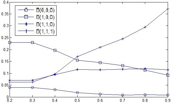
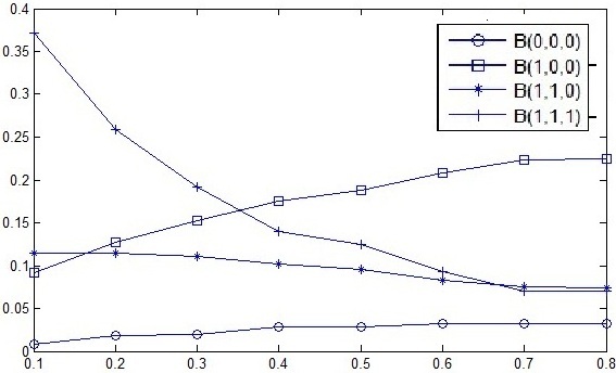
First, we consider the effect of λ0\lambda_{0} and λ1\lambda_{1}. Let |𝚽a||\bm{\Phi}_{a}| denote the volume of 𝚽a\bm{\Phi}_{a} , define the normalized volume |𝚽a|/|𝕏||\bm{\Phi}_{a}|/|\mathbb{X}| as the volume of 𝚽a\bm{\Phi}_{a} normalized against the volume of the total belief space 𝕏\mathbb{X} . Due to the symmetry property of the decision regions, we only study the decision regions for the following 4 actions (0,0,0),(1,0,0),(1,1,0),(1,1,1)(0,0,0),(1,0,0),(1,1,0),(1,1,1). For ease of notation, in the following discussion we use B0B_{0}, B1B_{1}, B2B_{2} and B3B_{3} to denote these four actions, respectively.

We first fix the value of λ1\lambda_{1} and increase λ0\lambda_{0} from 0.1 to 0.8. Fig. 5a shows the normalized volume of the four decision regions with increasing λ0\lambda_{0}. We can see that initially when λ0=0.1\lambda_{0}=0.1, 𝚽B3\bm{\Phi}_{B_{3}} has the biggest volume, it then decreases rapidly when λ0\lambda_{0} increases. The volume of 𝚽B1\bm{\Phi}_{B_{1}} also changes significantly with increasing λ0\lambda_{0}, but in contrast to 𝚽B3\bm{\Phi}_{B_{3}}, it increases rapidly when λ0\lambda_{0} increases. When λ0=0.8\lambda_{0}=0.8, 𝚽B1\bm{\Phi}_{B_{1}} has the biggest volume. This trends have the following implications: when λ0\lambda_{0} is small, which means the channels tend to remain in the bad state, it is beneficial to allocate power to all the channels (choose action B3=(1,1,1)B_{3}=(1,1,1)), whilst when λ0\lambda_{0} is large, which means the channel is very likely to change from bad state to good state, it is better to “gamble” on one channel (choose action B1=(1,0,0)B_{1}=(1,0,0)).

Similar trends can be observed in Fig. 5b which shows the volumes of the four decision regions versus λ1\lambda_{1}. When λ1\lambda_{1} is small, 𝚽B1\bm{\Phi}_{B_{1}} has the biggest value, which means it is optimal to “bet” on one channel when λ1\lambda_{1} is small. When λ1\lambda_{1} is greater than 0.490.49, 𝚽B3\bm{\Phi}_{B_{3}} overtakes 𝚽B1\bm{\Phi}_{B_{1}}, which means when λ1\lambda_{1} is big enough it is better for the system to take a more conservative action by allocating power to all the channels instead of “gambling” on one channel. The interesting thing is that |𝚽B0||\bm{\Phi}_{B_{0}}| and |𝚽B2||\bm{\Phi}_{B_{2}}| change only slightly with varying λ0\lambda_{0} and λ1\lambda_{1}. This implies that in order to maximize the reward, the system should either allocate the transmission power to all the channels or gamble on one channel. Using part of the channels (B2=(1,1,0)B_{2}=(1,1,0)) or doing nothing (B0=(0,0,0)B_{0}=(0,0,0)) is always not a good idea to maximize the long term reward.
Refer to caption
(a) λ0\lambda_{0}
Refer to caption
(b) λ1\lambda_{1}
Fig. 5: Normalized |𝚽a||\bm{\Phi}_{a}| with varying λ0\lambda_{0}, λ1\lambda_{1} (R1=3,R2=1.75,R3=1.361,RkCk=2R_{1}=3,R_{2}=1.75,R_{3}=1.361,\frac{R_{k}}{C_{k}}=2)

Next we study the effect of immediate reward RkR_{k} and immediate loss Ck​(1≤k≤N)C_{k}\>(1\leq k\leq N) on the structure of the optimal policy. It is straightforward to think that if the ratio of Rk/CkR_{k}/C_{k} is large, the total system reward will be large. Fig. 6 shows that when Rk/CkR_{k}/C_{k} grows, the normalized volume of 𝚽B0\bm{\Phi}_{B_{0}} and 𝚽B3\bm{\Phi}_{B_{3}} decreases, whist 𝚽B1\bm{\Phi}_{B_{1}} grows with Rk/CkR_{k}/C_{k}. 𝚽B2\bm{\Phi}_{B_{2}} decreases at first and then increases. For all four actions, the volumes of the decision regions reach a constant level respectively and remain unchanged when Rk/CkR_{k}/C_{k} grows beyond a certain value.

Refer to caption
(a) B0B_{0}
Refer to caption
(b) B1B_{1}
Refer to caption
(c) B2B_{2}
Refer to caption
(d) B3B_{3}
Fig. 6: Normalized |𝚽a||\bm{\Phi}_{a}| vs. Rk/Ck​(1≤k≤N)R_{k}/C_{k}\>(1\leq k\leq N) (R1=3,R2=1.55,R3=1.06,λ0=0.1,λ1=0.9R_{1}=3,R_{2}=1.55,R_{3}=1.06,\lambda_{0}=0.1,\lambda_{1}=0.9)

In fact, we notice in Fig. 6 that the value of Rk/CkR_{k}/C_{k} have limited effect on the decision regions in terms of percentage of each decision region in the whole belief space. Now we consider the value of k2​Rk2k1​Rk1\frac{k_{2}R_{k_{2}}}{k_{1}R_{k_{1}}} and k2​Ck2k1​Ck1\frac{k_{2}C_{k_{2}}}{k_{1}C_{k_{1}}} , and try to find out how they affect the structure of optimal policy (here we fix the value of Rk/CkR_{k}/C_{k}, so k2​Ck2k1​Ck1\frac{k_{2}C_{k_{2}}}{k_{1}C_{k_{1}}} changes along with k2​Rk2k1​Rk1\frac{k_{2}R_{k_{2}}}{k_{1}R_{k_{1}}} in the same manner). As in Section III, we assume that Rk2<Rk1<k2​Rk2/k1R_{k_{2}}<R_{k_{1}}<k_{2}R_{k_{2}}/k_{1}, Ck2<Ck1<k2​Ck2/k1C_{k_{2}}<C_{k_{1}}<k_{2}C_{k_{2}}/k_{1} and Rk>Ck​(1≤k1≤k2≤M)R_{k}>C_{k}(1\leq k_{1}\leq k_{2}\leq M), so that when more channels are chosen in an action, the system obtains larger immediate reward k​RkkR_{k}, therefore our power allocation scheme encourages the system to allocate power to more channels. It is shown in Fig. 7 that when k2​Rk2k1​Rk1\frac{k_{2}R_{k_{2}}}{k_{1}R_{k_{1}}} grows, normalized |𝚽B1||\bm{\Phi}_{B_{1}}| decreases whilst |𝚽B3||\bm{\Phi}_{B_{3}}| increases. Therefore when k2​Rk2k1​Rk1\frac{k_{2}R_{k_{2}}}{k_{1}R_{k_{1}}} is large, the total immediate reward is large enough for the system to act conservatively by allocating the transmission power to all the channels. Whilst when k2​Rk2k1​Rk1\frac{k_{2}R_{k_{2}}}{k_{1}R_{k_{1}}} is small, the total immediate reward is so small that system would rather “gamble” on one channel. Like the observation in Fig.6, the values of |𝚽B0||\bm{\Phi}_{B_{0}}| and |𝚽B2||\bm{\Phi}_{B_{2}}| only change slightly with varying k2​Rk2k1​Rk1\frac{k_{2}R_{k_{2}}}{k_{1}R_{k_{1}}}.

Refer to caption
(a) B0B_{0}
Refer to caption
(b) B1B_{1}
Refer to caption
(c) B2B_{2}
Refer to caption
(d) B3B_{3}
Fig. 7: Normalized |𝚽a||\bm{\Phi}_{a}| with changing k2​Rk2k1​Rk1\frac{k_{2}R_{k_{2}}}{k_{1}R_{k_{1}}} (λ0=0.1,λ1=0.9,R1=3,C1=1.5\lambda_{0}=0.1,\lambda_{1}=0.9,R_{1}=3,C_{1}=1.5)

From the discussion above, we can draw a conclusion that: when λ1−λ0\lambda_{1}-\lambda_{0} and k2​Rk2k1​Rk1\frac{k_{2}R_{k_{2}}}{k_{1}R_{k_{1}}} are large, the system tends to act conservatively and share power among all the channels; when λ1−λ0\lambda_{1}-\lambda_{0} and k2​Rk2k1​Rk1\frac{k_{2}R_{k_{2}}}{k_{1}R_{k_{1}}} are small, the system tends to “gamble” on one channel. No matter how the parameters change, action B2B_{2} is a mediocre choice and bring medium reward thus this action is not often taken. Action B0B_{0} is seldom chosen by the system since it brings no immediate reward, it is chosen only when the belief is so small that the system is almost sure to suffer loss.

V Conclusion

In this paper, we have studied the power allocation problem over N⁡(N≥3)N(N\geq 3) Gilbert-Elliott channels. We have theoretically derived the threshold-based structure of the optimal policy for N=3N=3, and graphically illustrated the structure by formulating and solving a linear programming formulation of the problem. For N>3N>3, it is difficult to demonstrate the results graphically, but it is possible to derive the structure mathematically, and we will work on this issue in the future. For future work, we would also like to investigate the case of non-identical channels and use a multi-armed bandit (MAB) formulation to find the thresholds for multiple channel system with N>3N>3.

Acknowledgment

This work is partially supported by National Key Basic Research Program of China under grant 2013CB329603, Natural Science Foundation of China under grant 61071081 and 60932003. This research was also sponsored in part by the U.S. Army Research Laboratory under the Network Science Collaborative Technology Alliance, Agreement Number W911NF-09-2-0053, and by the Okawa Foundation, under an Award to support research on ¡°Network Protocols that Learn¡±.

References

  • [1] A. J. Goldsmith and S. Chua, “Variable-rate variable-power MQAM for fading channels”, IEEE Trans. Commun., vol. 45, pp. 1218-1230, Oct. 1997.
  • [2] E. N. Gilbert, “Capacity of a burst-noise channel,” Bell Syst. Tech. J., vol. 39, pp. 1253-1265, Sep. 1960.
  • [3] L. Johnston and V. Krishnamurthy, “Opportunistic file transfer over a fading channel¡ªa POMDP search theory formulation with optimal threshold policies,” IEEE Trans. Wireless Commun., vol. 5, no. 2, pp. 394-405, Feb. 2006.
  • [4] D. Zhang and K. M. Wasserman, “Transmission schemes for time-varying wireless channels with partial state observations,” Proc. INFOCOM, pp. 467-476, 2002.
  • [5] I. Zaidi and V. Krishnamurthy, “Stochastic adaptive multilevel waterfilling in MIMO-OFDM WLANs,” 39th Asilomar Conference on Signals, Systems and Computers, 2005.
  • [6] X. Wang, D. Wang, H. Zhuang, and S. D. Morgera, “Energy-efficient resource allocation in wireless sensor networkds over fading TDMA channels,” IEEE Journal on Selected Areas in Communications (JSAC), vol. 28, no. 7, pp.1063-1072, 2010.
  • [7] Y. Gai and B. Krishnamachari, “Online learning algorithms for stochastic water-filling,” Information Theory and Application Workshop (ITA 2012), 2012.
  • [8] A. Laourine and L. Tong, “Betting on gilbert-elliot channels,” IEEE Transactions on Wireless communications, vol. 9, pp. 723-733, February 2010.
  • [9] Y. Wu and B. Krishnamachari, “Online learning to optimize transmission over unknown gilbert-elliott channel,” WiOpt, 2012.
  • [10] J. Tang, P. Mansourifard, and B. Krishnamachari, “Power allocation over two identical gilbert-elliott channels,” ICC 2013, June 2013.
  • [11] W. Jiang, J. Tang, and B. Krishnamachari, “Optimal Power allocation Policy over two identical gilbert-elliott channels,” ICC 2013, June 2013.
  • [12] R. D. Smallwood and E. J. Sondik, “The optimal control of partially observable markov processes over a finite horizon,” Operations Research, vol. 21, pp. 1071¨C1088, September-October 1973.
  • [13] S. M. Ross, Applied Probability Models with Optimization Applications. San Francisco: Holden-Day, 1970.
  • [14] D. P. D. Farias and B. V. Roy, “The linear programming approach to approximate dynamic programming,” Operations Research, vol. 51, pp. 850-865, November-December 2002.
  • [15] “Neos server for optimization.” http://neos.mcs.anl.gov/neos/.
  • [16] R. Fourer, D. M. Gay, and B. W. Kernighan, AMPL: A Modeling Language for Mathematical Programming. Brooks/Cole Publishing Company, 2002.