Living on the edge: Phase transitions
in convex programs with random data

Dennis Amelunxen , Martin Lotz , Michael B. Mccoy and Joel A. Tropp

Date: 26 March 2013. Revised 26 January 2014 and 24 April 2014.

Abstract.

Recent research indicates that many convex optimization problems with random constraints exhibit a phase transition as the number of constraints increases. For example, this phenomenon emerges in the $\ell_{1}$ minimization method for identifying a sparse vector from random linear measurements. Indeed, the $\ell_{1}$ approach succeeds with high probability when the number of measurements exceeds a threshold that depends on the sparsity level; otherwise, it fails with high probability.

This paper provides the first rigorous analysis that explains why phase transitions are ubiquitous in random convex optimization problems. It also describes tools for making reliable predictions about the quantitative aspects of the transition, including the location and the width of the transition region. These techniques apply to regularized linear inverse problems with random measurements, to demixing problems under a random incoherence model, and also to cone programs with random affine constraints.

The applied results depend on foundational research in conic geometry. This paper introduces a summary parameter, called the statistical dimension, that canonically extends the dimension of a linear subspace to the class of convex cones. The main technical result demonstrates that the sequence of intrinsic volumes of a convex cone concentrates sharply around the statistical dimension. This fact leads to accurate bounds on the probability that a randomly rotated cone shares a ray with a fixed cone.

2010 Mathematics Subject Classification

Primary: 90C25, 52A22, 60D05. Secondary: 52A20, 62C20.

1. Motivation

A phase transition is a sharp change in the character of a computational problem as its parameters vary. Recent research suggests that phase transitions emerge in many random convex optimization problems from mathematical signal processing and computational statistics; for example, see [DT09b, Sto09, OH10, CSPW11, DGM13, MT14b]. This paper proves that the locations of these phase transitions are determined by geometric invariants associated with the mathematical programs. Our analysis provides the first complete account of transition phenomena in random linear inverse problems, random demixing problems, and random cone programs.

1.1. Vignette: Compressed sensing

To illustrate our goals, we discuss the compressed sensing problem, a familiar example where a phase transition is plainly visible in numerical experiments [DT09b]. Let $\bm{x}_{0}\in\mathbb{R}^{d}$ be an unknown vector with $s$ nonzero entries. Let $\bm{A}$ be an $m\times d$ random matrix whose entries are independent standard normal variables, and suppose we have access to the vector

\bm{z}_{0}=\bm{A}\bm{x}_{0}\in\mathbb{R}^{m}.

(1.1)

This serves as a model for data acquisition: we interpret $\bm{z}_{0}$ as a collection of $m$ independent linear measurements of the unknown $\bm{x}_{0}$ . The compressed sensing problem requires us to identify $\bm{x}_{0}$ given only the measurement vector $\bm{z}_{0}$ and the realization of the measurement matrix $\bm{A}$ . When the number $m$ of measurements is smaller than the ambient dimension $d$ , we cannot solve this inverse problem unless we take advantage of the prior knowledge that $\bm{x}_{0}$ is sparse.

The method of $\ell_{1}$ minimization [CDS01, CT06, Don06a] is a well-established approach to the compressed sensing problem. This technique searches for the sparse unknown $\bm{x}_{0}$ by solving the convex program

\text{minimize}\quad\left\|{\bm{x}}\right\|_{1}\quad\text{subject to}\quad\bm{z}_{0}=\bm{A}\bm{x},

(1.2)

where $\left\|{\bm{x}}\right\|_{1}:=\sum_{i=1}^{d}\left|{x_{i}}\right|$ . This approach is sensible because the $\ell_{1}$ norm of a vector can serve as a proxy for the sparsity. We say that (1.2) succeeds at solving the compressed sensing problem when it has a unique optimal point $\widehat{\bm{x}}$ and $\widehat{\bm{x}}$ equals the true unknown $\bm{x}_{0}$ ; otherwise, it fails.

Figure 1.1 depicts the results of a computer experiment designed to estimate the probability that (1.2) succeeds as we vary the sparsity $s$ of the unknown $\bm{x}_{0}$ and the number $m$ of random measurements. We consider two choices for the ambient dimension, $d=100$ and $d=600$ . For each choice of $s$ and $m$ , we construct a vector $\bm{x}_{0}$ with $s$ nonzero entries, we draw $m$ random measurements according to the model (1.1), and we solve the problem (1.2). The brightness of the point $(s,m)$ indicates the probability of success, estimated from $50$ independent trials. White represents certain success, while black represents certain failure. The plot evinces that, for a given sparsity level $s$ , the $\ell_{1}$ minimization technique (1.2) almost always succeeds when we have an adequate number $m$ of measurements, while it almost always fails when we have fewer measurements. Appendix A contains more details about this experiment.

Refer to caption — Figure 1.1. The phase transition phenomenon in compressed sensing. This diagram shows the empirical probability that the $\ell_{1}$ minimization method (1.2) successfully identifies a vector $\bm{x}_{0}\in\mathbb{R}^{d}$ with $s$ nonzero entries given a vector $\bm{z}_{0}$ consisting of $m$ random measurements of the form $\bm{z}_{0}=\bm{A}\bm{x}_{0}$ where $\bm{A}$ is an $m\times d$ matrix with independent standard normal entries. The brightness of each point reflects the observed probability of success, ranging from certain failure (black) to certain success (white). [left] The ambient dimension $d=100$ . [right] The ambient dimension $d=600$ .

Figure 1.1 raises several interesting questions about the performance of the $\ell_{1}$ minimization method (1.2) for solving the compressed sensing problem:

•

What is the probability of success? For a given pair $(s,m)$ of parameters, can we estimate the probability that (1.2) succeeds or fails?
•

Does a phase transition exist? Is there a simple curve $m=\psi(s)$ that separates the parameter space into regions where (1.2) is very likely to succeed or to fail?
•

Where is the edge of the phase transition? Can we find a formula for the location of this threshold between success and failure?
•

How wide is the transition region? For a given sparsity level $s$ and ambient dimension $d$ , how big is the range of $m$ where the probability of success and failure are comparable?
•

Why does the transition exist? Is there a geometric explanation for the phase transition in compressed sensing? Can we export this reasoning to understand other problems?

There is an extensive body of work dedicated to these questions and their relatives. See the books [EK12, FR13] for background on compressed sensing in general. Section 10 outlines the current state of knowledge about phase transitions in convex optimization methods for signal processing. In spite of all this research, a complete explanation of these phenomena is lacking. The goal of this paper is to answer the questions we have posed.

1.2. Notation

Before moving forward, let us introduce some notation. We use standard conventions from convex analysis, as set out in Rockafellar [Roc70]. For vectors $\bm{x},\bm{y}\in\mathbb{R}^{d}$ , we define the Euclidean inner product $\left\langle{\bm{x}},\ {\smash{\bm{y}}}\right\rangle:=\sum_{i=1}^{d}x_{i}y_{i}$ and the squared Euclidean norm $\left\|{\bm{x}}\right\|^{2}:=\left\langle{\bm{x}},\ {\bm{x}}\right\rangle$ . The Euclidean distance to a set $S\subset\mathbb{R}^{d}$ is the function

\dist(\cdot,S):\mathbb{R}^{d}\to\mathbb{R}_{+}\quad\text{where}\quad\dist(\bm{x},S):=\inf\big\{\left\|{\smash{\bm{x}-\bm{y}}}\right\|:\bm{y}\in S\big\}

and $\mathbb{R}_{+}$ denotes the set of nonnegative real numbers. The unit ball $\mathsf{B}^{d}$ and unit sphere $\mathsf{S}^{d-1}$ in $\mathbb{R}^{d}$ are the sets

\mathsf{B}^{d}:=\big\{\bm{x}\in\mathbb{R}^{d}:\left\|{\bm{x}}\right\|\leq 1\big\}\quad\text{and}\quad\mathsf{S}^{d-1}:=\big\{\bm{x}\in\mathbb{R}^{d}:\left\|{\bm{x}}\right\|=1\big\}.

An orthogonal basis $\bm{U}\in\mathbb{R}^{d\times d}$ for $\mathbb{R}^{d}$ is a matrix that satisfies $\bm{U}^{T}\bm{U}=\mathbf{I}$ , where $\mathbf{I}$ is the identity.

A convex cone $C\subset\mathbb{R}^{d}$ is a convex set that is positively homogeneous: $C=\tau C$ for all $\tau>0$ . Let us emphasize that the vertex of a convex cone is always located at the origin. For a closed convex cone $C$ , the Euclidean projection $\bm{\Pi}_{C}(\bm{x})$ of a point $\bm{x}$ onto the cone returns the point in $C$ nearest to $\bm{x}$ :

\bm{\Pi}_{C}(\bm{x}):=\operatorname*{arg\;min}\big\{\left\|{\smash{\bm{x}-\bm{y}}}\right\|:\bm{y}\in C\big\}.

(1.3)

For a general cone $C\subset\mathbb{R}^{d}$ , the polar cone $C^{\circ}$ is the set of outward normals of $C$ :

C^{\circ}:=\big\{\bm{u}\in\mathbb{R}^{d}:\left\langle{\bm{u}},\ {\bm{x}}\right\rangle\leq 0\quad\text{for all $\bm{x}\in C$}\big\}.

(1.4)

The polar cone $C^{\circ}$ is always closed and convex.

We make heavy use of probability in this work. The symbol $\mathbb{P}\{\cdot\}$ denotes the probability of an event, and $\operatorname{\mathbb{E}}[\cdot]$ returns the expectation of a random variable. We reserve the letter $\bm{g}$ for a standard normal random vector, i.e., a vector whose entries are independent Gaussian random variables with mean zero and variance one. We reserve the letter $\bm{\theta}$ for a random vector uniformly distributed on the Euclidean unit sphere. The set of orthogonal matrices forms a compact Lie group, so it admits an invariant Haar (i.e., uniform) probability measure. We reserve the letter $\bm{Q}$ for a uniformly random orthogonal matrix, and we refer to $\bm{Q}$ as a random orthogonal basis or a random rotation.

2. Conic geometry and phase transitions

In the theory of convex analysis, convex cones take over the central role that subspaces perform in linear algebra [HUL93, p. 90]. In particular, we can use convex cones to express the optimality conditions for a convex program [HUL93, Part VII]. When a convex optimization problem includes random data, the optimality conditions may involve random convex cones. Therefore, the study of random convex optimization problems leads directly to questions about the stochastic geometry of cones.

This perspective is firmly established in the literature on convex optimization for signal processing applications. Rudelson & Vershynin [RV08, Sec. 4] analyze the $\ell_{1}$ minimization method (1.2) for the compressed sensing problem by examining the conic formulation of the optimality conditions. They apply deep results [Gor85, Gor88] for Gaussian processes to bound the probability that $\ell_{1}$ minimization succeeds. Many subsequent papers, including [Sto09, OH10, CRPW12], rely on the same argument.

In sympathy with these prior works, we study random convex optimization problems by considering the conic formulation of the optimality conditions. In contrast, we have developed a new technical argument to study the probability that the conic optimality conditions hold. Our approach depends on exact formulas from the field of conic integral geometry [SW08, Chap. 6.5]. In this context, the general idea of using integral geometry is due to Donoho [Don06b] and Donoho & Tanner [DT09a]. The specific method in this paper was proposed in [MT14b], but we need to install additional machinery to prove that phase transitions occur.

Sections 2.1–2.4 outline the results we need from conic integral geometry, along with our contributions to this subject. We apply this theory in Sections 2.5 and 2.6 to study some random optimization problems. We conclude with a summary of our main results in Section 2.7.

2.1. The kinematic formula for cones

Let us begin with a beautiful and classical problem from the field of conic integral geometry:

What is the probability that a randomly rotated convex cone shares a ray with a fixed convex cone?

See Figure 2.1 for an illustration of the geometry. Formally, we consider convex cones $C$ and $K$ in $\mathbb{R}^{d}$ , and we draw a random orthogonal basis $\bm{Q}\in\mathbb{R}^{d\times d}$ . The goal is to find a useful expression for the probability

\mathbb{P}\big\{C\cap\bm{Q}K\neq\{\bm{0}\}\big\}.

As we will discuss, this is the key question we must answer to understand phase transition phenomena in convex optimization problems with random data.

In two dimensions, we quickly determine the solution to the problem. Consider two convex cones $C$ and $K$ in $\mathbb{R}^{2}$ . If neither cone is a linear subspace, then

\mathbb{P}\big\{C\cap\bm{Q}K\neq\{\bm{0}\}\big\}=\min\big\{v_{2}(C)+v_{2}(K),\ 1\big\},

where $v_{2}(\cdot)$ returns the proportion of the unit circle subtended by (the closure of) a convex cone in $\mathbb{R}^{2}$ . A similar formula holds when one of the cones is a subspace. In higher dimensions, however, convex cones can be complicated objects. In three dimensions, the question already starts to look difficult, and we might despair that a reasonable solution exists in general.

Figure 2.1. Randomly rotated convex cones. Let

C

and

K

be nontrivial convex cones, and let

\bm{Q}

be a random orthogonal basis. The cone

C

is fixed, and

\bm{Q}K

is a randomly rotated copy of

K

. [left] The two cones have a trivial intersection. [right] The two cones share a ray.

It turns out that there is an exact formula for the probability that a randomly rotated convex cone shares a ray with a fixed convex cone. Moreover, in $d$ dimensions, we only need $d+1$ numbers to summarize each cone. This wonderful result is called the conic kinematic formula [SW08, Thm. 6.5.6]. We record the statement here, but you should not focus on the details at this stage; Section 5 contains a more thorough presentation.

Fact 2.1 (The kinematic formula for cones).

Let $C$ and $K$ be closed convex cones in $\mathbb{R}^{d}$ , one of which is not a subspace. Draw a random orthogonal basis $\bm{Q}\in\mathbb{R}^{d\times d}$ . Then

\mathbb{P}\big\{C\cap\bm{Q}K\neq\{\bm{0}\}\big\}=\sum_{i=0}^{d}\big(1+(-1)^{i+1}\big)\sum_{j=i}^{d}v_{i}(C)\cdot v_{d+i-j}(K).

For each $k=0,1,2,\dots,d$ , the geometric functional $v_{k}$ maps a closed convex cone to a nonnegative number, called the $k$ th intrinsic volume of the cone.

The papers [AB12, MT14b] have recognized that the conic kinematic formula is tailor-made for studying random instances of convex optimization problems. Unfortunately, this approach suffers a serious weakness: We do not have workable expressions for the intrinsic volumes of a cone, except in the simplest cases. This paper provides a way to make the kinematic formula effective. To explain, we need to have a closer look at the conic intrinsic volumes.

2.2. Concentration of intrinsic volumes and the statistical dimension

The conic intrinsic volumes, introduced in Fact 2.1, are the fundamental geometric invariants of a closed convex cone. They do not depend on the dimension of the space in which the cone is embedded, nor on the orientation of the cone within that space. For an analogy in Euclidean geometry, you may consider similar quantities defined for compact convex sets, such as the usual volume, the surface area, the mean width, and the Euler characteristic [Sch93].

We will provide a more rigorous treatment of the conic intrinsic volumes in Section 5. For now, the only formal property we need is that the intrinsic volumes of a closed convex cone $C$ in $\mathbb{R}^{d}$ compose a probability distribution on $\{0,1,2,\dots,d\}$ . That is,

\sum_{k=0}^{d}v_{k}(C)=1\quad\text{and}\quad v_{k}(C)\geq 0\quad\text{for $k=0,1,2,\dots,d$.}

Figure 2.2 displays the distribution of intrinsic volumes for a particular cone; you can see that the sequence has a sharp peak at its mean value. Our work establishes a remarkable new fact about conic geometry:

For every closed convex cone, the distribution of conic intrinsic volumes concentrates sharply around its mean value.

This result is our main technical achievement; Theorem 6.1 contains a precise statement.

Figure 2.2. Concentration of conic intrinsic volumes. This plot displays the conic intrinsic volumes

v_{k}(C)

of a circular cone

C\subset\mathbb{R}^{128}

with angle

\pi/6

. The distribution concentrates sharply around the statistical dimension

\delta(C)\approx 32.5

. See Section 3.4 for further discussion of this example.

Because of the concentration phenomenon, the mean value of the distribution of conic intrinsic volumes serves as a summary for the entire distribution. This insight leads to the central definition of the paper.

Definition 2.2 (Statistical dimension: Intrinsic characterization).

Let $C$ be a closed convex cone in $\mathbb{R}^{d}$ . The statistical dimension $\delta(C)$ of the cone is defined as

\delta(C):=\sum_{k=0}^{d}k\,v_{k}(C).

The statistical dimension of a general convex cone is the statistical dimension of its closure.

As the name suggests, the statistical dimension reflects the dimensionality of a convex cone. Here are some properties that support this interpretation. First, the statistical dimension increases with the size of a cone. Indeed, for nested convex cones $C\subset K\subset\mathbb{R}^{d}$ , we have the inequalities $0\leq\delta(C)\leq\delta(K)\leq d$ . Second, the statistical dimension of a linear subspace $L$ always satisfies

\delta(L)=\dim(L).

(2.1)

In fact, the statistical dimension is a canonical extension of the dimension of a linear subspace to the class of convex cones! Section 5.6 provides technical justification for the latter point, while Sections 3, 4, and 5 establish various properties of the statistical dimension.

2.3. The approximate kinematic formula

We can simplify the conic kinematic formula, Fact 2.1, by exploiting the concentration of intrinsic volumes.

Theorem I (Approximate kinematic formula).

Fix a tolerance $\eta\in(0,1)$ . Let $C$ and $K$ be convex cones in $\mathbb{R}^{d}$ , and draw a random orthogonal basis $\bm{Q}\in\mathbb{R}^{d\times d}$ . Then

	$\displaystyle\delta(C)+\delta(K)\leq d-a_{\eta}\sqrt{d}$	$\displaystyle\quad\Longrightarrow\quad\mathbb{P}\big\{C\cap\bm{Q}K\neq\{\bm{0}\}\big\}\leq\eta;$
	$\displaystyle\delta(C)+\delta(K)\geq d+a_{\eta}\sqrt{d}$	$\displaystyle\quad\Longrightarrow\quad\mathbb{P}\big\{C\cap\bm{Q}K\neq\{\bm{0}\}\big\}\geq 1-\eta.$

The quantity $a_{\eta}:=\sqrt{8\log(4/\eta)}$ . For example, $a_{0.01}<7$ and $a_{0.001}<9$ .

In Section 7, we derive Theorem I along with some more precise results.

Theorem I says that two randomly rotated cones are likely to share a ray if and only if the total statistical dimension of the two cones exceeds the ambient dimension. This statement is in perfect sympathy with the analogous result for random subspaces. We extract the following lesson:

We can assign a dimension $\delta(C)$ to each convex cone $C$ . For problems in conic integral geometry, the cone behaves much like a subspace with approximate dimension $\delta(C)$ .

In Sections 2.5 and 2.6, we use Theorem I to prove that a large class of random convex optimization problems always exhibits a phase transition, and we demonstrate that the statistical dimension describes the location of the phase transition.

Remark 2.3 (Gaussian process theory).

If we replace the random orthogonal basis in Theorem I with a standard normal matrix, we obtain a different problem in stochastic geometry. For the Gaussian model, we can establish a partial analog of Theorem I using a comparison inequality for Gaussian processes [Gor85, Thm. 1.4]. Rudelson & Vershynin [RV08, Sec. 4] have used a corollary [Gor88] of this result to study the $\ell_{1}$ minimization method (1.2) for compressed sensing. Many subsequent papers, including [Sto09, OH10, CRPW12], depend on the same argument. In contrast to Theorem I, this approach is not based on an exact formula. Nor does it apply to the random orthogonal model, which is more natural than the Gaussian model for many applications.

2.4. Calculating the statistical dimension

The statistical dimension arises from deep considerations in conic integral geometry, and we rely on this connection to prove that phase transitions occur in random convex optimization problems. There is an alternative formulation that is often useful for calculating the statistical dimension of specific cones.

Proposition 2.4 (Statistical dimension: Metric characterization).

The statistical dimension $\delta(C)$ of a closed convex cone $C$ in $\mathbb{R}^{d}$ satisfies

\delta(C)=\operatorname{\mathbb{E}}\big[\left\|{\smash{\bm{\Pi}_{C}(\bm{g})}}\right\|^{2}\big],

(2.2)

where $\bm{g}\in\mathbb{R}^{d}$ is a standard normal vector, $\left\|{\cdot}\right\|$ is the Euclidean norm, and $\bm{\Pi}_{C}$ denotes the Euclidean projection (1.3) onto the cone $C$ .

The proof of Proposition 2.4 appears in Section 5.5. The argument requires a classical result called the spherical Steiner formula [SW08, Thm. 6.5.1].

The metric characterization of the statistical dimension provides a surprising link between two perspectives on random convex optimization problems: our approach based on integral geometry and the alternative approach based on Gaussian process theory. Indeed, the formula (2.2) is closely related to the definition of another summary parameter for convex cones called the Gaussian width; see Section 10.3 for more information. This connection allows us to perform statistical dimension calculations by adapting methods [RV08, Sto09, OH10, CRPW12] developed for the Gaussian width.

We undertake this program in Sections 3 and 4 to estimate the statistical dimension for several important families of convex cones. Although the resulting formulas are not substantially novel, we prove for the first time that the error in these calculations is negligible. Our contribution to this analysis forms a critical part of the rigorous computation of phase transitions.

2.5. Regularized linear inverse problems with a random model

Our first application of Theorem I concerns a generalization of the compressed sensing problem that has been studied in [CRPW12]. A linear inverse problem asks us to infer an unknown vector $\bm{x}_{0}\in\mathbb{R}^{d}$ from an observed vector $\bm{z}_{0}\in\mathbb{R}^{m}$ of the form

\bm{z}_{0}=\bm{A}\bm{x}_{0},

(2.3)

where $\bm{A}\in\mathbb{R}^{m\times d}$ is a matrix that describes a linear data acquisition process. When the matrix is fat $(m<d)$ , the inverse problem is underdetermined. In this situation, we cannot hope to identify $\bm{x}_{0}$ unless we take advantage of prior information about its structure.

2.5.1. Solving linear inverse problems with convex optimization

Suppose that $f:\mathbb{R}^{d}\to\overline{\mathbb{R}}$ is a proper convex function¹¹ 1 The extended real numbers $\overline{\mathbb{R}}:=\mathbb{R}\cup\{\pm\infty\}$ . A proper convex function has at least one finite value and never takes the value $-\infty$ . that reflects the amount of “structure” in a vector. We can attempt to identify the structured unknown $\bm{x}_{0}$ in (2.3) by solving a convex optimization problem:

\text{minimize}\quad f(\bm{x})\quad\text{subject to}\quad\bm{z}_{0}=\bm{A}\bm{x}.

(2.4)

The function $f$ is called a regularizer, and the formulation (2.4) is called a regularized linear inverse problem. To illustrate the kinds of regularizers that arise in practice, we highlight two familiar examples.

Example 2.5 (Sparse vectors).

When the vector $\bm{x}_{0}$ is known to be sparse, we can minimize the $\ell_{1}$ norm to look for a sparse solution to the inverse problem. Repeating (1.2), we have the optimization

\text{minimize}\quad\left\|{\bm{x}}\right\|_{1}\quad\text{subject to}\quad\bm{z}_{0}=\bm{A}\bm{x}.

(2.5)

This approach was proposed by Chen et al. [CDS01], motivated by work in geophysics [CM73, SS86].

Example 2.6 (Low-rank matrices).

Suppose that $\bm{X}_{0}$ is a low-rank matrix, and we have acquired a vector of measurements of the form $\bm{z}_{0}=\mathscr{A}(\bm{X}_{0})$ , where $\mathscr{A}$ is a linear operator. This process is equivalent with (2.3). We can look for low-rank solutions to the linear inverse problem by minimizing the Schatten 1-norm:

\text{minimize}\quad\left\|{\bm{X}}\right\|_{S_{1}}\quad\text{subject to}\quad\bm{z}_{0}=\mathscr{A}(\bm{X}).

(2.6)

This method was proposed in [RFP10], based on ideas from control [MP97] and optimization [Faz02].

We say that the regularized linear inverse problem (2.4) succeeds at solving (2.3) when the convex program has a unique minimizer $\widehat{\bm{x}}$ that coincides with the true unknown; that is, $\widehat{\bm{x}}=\bm{x}_{0}$ . To develop conditions for success, we introduce a convex cone associated with the regularizer $f$ and the unknown $\bm{x}_{0}$ .

Definition 2.7 (Descent cone).

The descent cone $\mathcal{D}(f,\bm{x})$ of a proper convex function $f:\mathbb{R}^{d}\to\overline{\mathbb{R}}$ at a point $\bm{x}\in\mathbb{R}^{d}$ is the conic hull of the perturbations that do not increase $f$ near $\bm{x}$ .

\mathcal{D}(f,\bm{x})\mathrel{\mathop{:}}=\bigcup_{\tau>0}\big\{\bm{y}\in\mathbb{R}^{d}:f(\bm{x}+\tau\bm{y})\leq f(\bm{x})\big\}.

The descent cones of a proper convex function are always convex, but they may not be closed. The descent cones of a smooth convex function are always halfspaces, so this concept inspires the most interest when the function is nonsmooth.

To characterize when the optimization problem (2.4) succeeds, we write the primal optimality condition in terms of the descent cone; cf. [RV08, Sec. 4] and [CRPW12, Prop. 2.1].

Fact 2.8 (Optimality condition for linear inverse problems).

Let $f$ be a proper convex function. The vector $\bm{x}_{0}$ is the unique optimal point of the convex program (2.4) if and only if $\mathcal{D}(f,\bm{x}_{0})\cap\operatorname{null}(\bm{A})=\{\bm{0}\}.$

Figure 2.3 illustrates the geometry of this optimality condition. Despite its simplicity, this result forges a crucial link between the convex optimization problem (2.4) and the theory of conic integral geometry.

Figure 2.3. The optimality condition for a regularized inverse problem. The condition for the regularized linear inverse problem (2.4) to succeed requires that the descent cone

\mathcal{D}(f,\bm{x}_{0})

and the null space

\operatorname{null}(\bm{A})

do not share a ray. [left] The regularized linear inverse problem succeeds. [right] The regularized linear inverse problem fails.

2.5.2. Linear inverse problems with random data

Our goal is to understand the power of convex regularization for solving linear inverse problems, as well as the limitations inherent in this approach. To do so, we consider the case where the measurements are generic. A natural modeling technique is to draw the measurement matrix $\bm{A}$ at random from the standard normal distribution on $\mathbb{R}^{m\times d}$ . In this case, the kernel of the matrix $\bm{A}$ is a randomly oriented subspace, so the optimality condition, Fact 2.8, requires us to calculate the probability that this random subspace does not share a ray with the descent cone.

The kinematic formula, Fact 2.1, gives an exact expression for the probability that (2.4) succeeds under the random model for $\bm{A}$ . By invoking the approximate kinematic formula, Theorem I, we reach a simpler result that allows us to identify a sharp transition in performance as the number $m$ of measurements varies.

Theorem II (Phase transitions in linear inverse problems with random measurements).

Fix a tolerance $\eta\in(0,1)$ . Let $\bm{x}_{0}\in\mathbb{R}^{d}$ be a fixed vector, and let $f:\mathbb{R}^{d}\to\overline{\mathbb{R}}$ be a proper convex function. Suppose $\bm{A}\in\mathbb{R}^{m\times d}$ has independent standard normal entries, and let $\bm{z}_{0}=\bm{A}\bm{x}_{0}$ . Then

	$\displaystyle m\leq\delta\big(\mathcal{D}(f,\bm{x}_{0})\big)-a_{\eta}\sqrt{d}$	$\displaystyle\quad\Longrightarrow\quad\text{\eqref{eq:lin-inv-gen} succeeds with probability~$\leq\eta$};$
	$\displaystyle m\geq\delta\big(\mathcal{D}(f,\bm{x}_{0})\big)+a_{\eta}\sqrt{d}$	$\displaystyle\quad\Longrightarrow\quad\text{\eqref{eq:lin-inv-gen} succeeds with probability~$\geq 1-\eta$.}$

The quantity $a_{\eta}:=\sqrt{8\log(4/\eta)}$ .

Proof.

The standard normal distribution on $\mathbb{R}^{m\times d}$ is invariant under rotation, so the null space $L=\operatorname{null}(\bm{A})$ is almost surely a uniformly random $(d-m)$ -dimensional subspace of $\mathbb{R}^{d}$ . According to (2.1), the statistical dimension $\delta(L)=d-m$ almost surely. The result follows immediately when we combine the optimality condition, Fact 2.8, and the kinematic bound, Theorem I. ∎

Under minimal assumptions, Theorem II proves that we always encounter a phase transition when we use the regularized formulation (2.4) to solve the linear inverse problem with random measurements. The transition occurs where the number of measurements equals the statistical dimension of the descent cone: $m=\delta\big(\mathcal{D}(f,\bm{x}_{0})\big)$ . The shift from failure to success takes place over a range of about $O(\sqrt{d})$ measurements.

Here is one way to think about this result. We cannot identify $\bm{x}_{0}\in\mathbb{R}^{d}$ from the observation $\bm{z}_{0}\in\mathbb{R}^{m}$ by solving the linear system $\bm{A}\bm{x}=\bm{z}_{0}$ because we only have $m$ equations. Under the random model for $\bm{A}$ , the regularization in (2.4) effectively adds $d-\delta\big(\mathcal{D}(f,\bm{x}_{0})\big)$ more equations to the system. Therefore, we can typically recover $\bm{x}_{0}$ when $m\geq\delta\big(\mathcal{D}(f,\bm{x}_{0})\big)$ . This interpretation accords with the heuristic that the statistical dimension measures the dimension of a cone.

There are several reasons that the conclusions of Theorem II are significant. The first implication provides evidence about the minimum amount of information we need before we can use the convex method (2.4) to solve the linear inverse problem. The second implication tells us that we can solve the inverse problem reliably once we have acquired this quantum of information. Furthermore, Theorem II allows us to compare the performance of different regularizers because we know exactly how many measurements each one requires.

Remark 2.9 (Prior work).

A variant of the success condition $m\geq\delta\big(\mathcal{D}(f,\bm{x}_{0})\big)+O(\sqrt{d})$ from Theorem II already appears in the literature [CRPW12, Cor. 3.3(1)]. This result depends on the argument of Rudelson & Vershynin [RV08, Sec. 4], which uses the “escape from the mesh” theorem [Gor88] to verify the optimality condition, Fact 2.8, for the optimization problem (2.4). There is some evidence that the success condition accurately describes the performance limit for (2.4) with random measurements. Stojnic [Sto09] presents analysis and experiments for the $\ell_{1}$ norm, while Oymak & Hassibi [OH10] study the Schatten 1-norm. Results from [DMM09b, Sec. 17] and [BLM13a] imply that Stojnic’s calculation is asymptotically sharp.

Nevertheless, the prior literature offers no hint that the statistical dimension determines the location of the phase transition for every convex regularizer. In fact, we can derive a variant of the failure condition from Theorem II by supplementing Rudelson & Vershynin’s approach with a polarity argument. A similar observation appeared in Stojnic’s paper [Sto13] after our work was released.

2.5.3. Computer experiments

We have performed some computer experiments to compare the theoretical and empirical phase transitions. Figure 2.4[left] shows the performance of (2.5) for identifying a sparse vector in $\mathbb{R}^{100}$ from random measurements. Figure 2.4[right] shows the performance of (2.6) for identifying a low-rank matrix in $\mathbb{R}^{30\times 30}$ from random measurements. In each case, the heat map indicates the observed probability of success with respect to the randomness in the measurement operator. The 5%, 50%, and 95% success isoclines are calculated from the data. We also draft the theoretical phase transition curve, promised by Theorem II, where the number $m$ of measurements equals the statistical dimension of the appropriate descent cone; the statistical dimension formulas are drawn from Sections 4.3 and 4.4. See Appendix A for the experimental protocol.

In both examples, the theoretical prediction of Theorem II coincides almost perfectly with the 50% success isocline. Furthermore, the phase transition takes place over a range of $O(\sqrt{d})$ values of $m$ , as promised. Although Theorem II does not explain why the transition region tapers at the bottom-left and top-right corners of each plot, we have established a more detailed version of Theorem I that allows us to predict this phenomenon as well; see Section 7.1.

2.6. Demixing problems with a random model

In a demixing problem [MT14b], we observe a superposition of two structured vectors, and we aim to extract the two constituents from the mixture. More precisely, suppose that we have acquired a vector $\bm{z}_{0}\in\mathbb{R}^{d}$ of the form

\bm{z}_{0}=\bm{x}_{0}+\bm{U}\bm{y}_{0}

(2.7)

where $\bm{x}_{0},\bm{y}_{0}\in\mathbb{R}^{d}$ are unknown and $\bm{U}\in\mathbb{R}^{d\times d}$ is a known orthogonal matrix. If we wish to identify the pair $(\bm{x}_{0},\bm{y}_{0})$ , we must assume that each component is structured to reduce the number of degrees of freedom. In addition, if the two types of structure are coherent (i.e., aligned with each other), it may be impossible to disentangle them, so it is expedient to include the matrix $\bm{U}$ to model the relative orientation of the two constituent signals.

2.6.1. Solving demixing problems with convex optimization

Suppose that $f$ and $g$ are proper convex functions on $\mathbb{R}^{d}$ that promote the structures we expect to find in $\bm{x}_{0}$ and $\bm{y}_{0}$ . Then we can frame the convex optimization problem

\text{minimize}\quad f(\bm{x})\quad\text{subject to}\quad g(\bm{y})\leq g(\bm{y}_{0})\quad\text{and}\quad\bm{z}_{0}=\bm{x}+\bm{U}\bm{y}.

(2.8)

In other words, we seek structured vectors $\bm{x}$ and $\bm{y}$ that are consistent with the observation $\bm{z}_{0}$ . This approach requires the side information $g(\bm{y}_{0})$ , so a Lagrangian formulation is sometimes more natural in practice [MT14b, Sec. 1.2.4]. Here are two concrete examples of the demixing program (2.8) that are adapted from the literature.

Example 2.10 (Sparse + sparse).

Suppose that the first signal $\bm{x}_{0}$ is sparse in the standard basis, and the second signal $\bm{U}\bm{y}_{0}$ is sparse in a known basis $\bm{U}$ . In this case, we can use $\ell_{1}$ norms to promote sparsity, which leads to the optimization

\text{minimize}\quad\left\|{\bm{x}}\right\|_{1}\quad\text{subject to}\quad\left\|{\smash{\bm{y}}}\right\|_{1}\leq\left\|{\smash{\bm{y}_{0}}}\right\|_{1}\quad\text{and}\quad\bm{z}_{0}=\bm{x}+\bm{U}\bm{y}.

(2.9)

This approach for demixing sparse signals is sometimes called morphological component analysis [SDC03, SED05, ESQD05, BMS06].

Example 2.11 (Low-rank + sparse).

Suppose that we observe $\bm{Z}_{0}=\bm{X}_{0}+\mathscr{U}(\bm{Y}_{0})$ where $\bm{X}_{0}$ is a low-rank matrix, $\bm{Y}_{0}$ is a sparse matrix, and $\mathscr{U}$ is a known orthogonal transformation on the space of matrices. We can minimize the Schatten 1-norm to promote low rank, and we can constrain the $\ell_{1}$ norm to promote sparsity. The optimization becomes

\text{minimize}\quad\left\|{\bm{X}}\right\|_{S_{1}}\quad\text{subject to}\quad\left\|{\bm{Y}}\right\|_{1}\leq\left\|{\bm{Y}_{0}}\right\|_{1}\quad\text{and}\quad\bm{Z}_{0}=\bm{X}+\mathscr{U}(\bm{Y}).

(2.10)

This demixing problem is called the rank–sparsity decomposition [CSPW11].

We say that the convex program (2.8) for demixing succeeds when it has a unique solution $(\widehat{\bm{x}},\widehat{\bm{y}})$ that coincides with the vectors that generate the observation: $(\widehat{\bm{x}},\widehat{\bm{y}})=(\bm{x}_{0},\bm{y}_{0})$ . As in the case of a linear inverse problem, we can express the primal optimality condition in terms of descent cones; cf. [MT14b, Lem. 2.4].

Fact 2.12 (Optimality condition for demixing).

Let $f$ and $g$ be proper convex functions. The pair $(\bm{x}_{0},\bm{y}_{0})$ is the unique optimal point of the convex program (2.8) if and only if $\mathcal{D}(f,\bm{x}_{0})\cap(-\bm{U}\mathcal{D}(g,\bm{y}_{0}))=\{\bm{0}\}$ .

Figure 2.5 depicts the geometry of this optimality condition. The parallel with Fact 2.8, the optimality condition for a regularized linear inverse problem, is striking. Indeed, the two conditions coalesce when the function $g$ in (2.8) is the indicator of an appropriate affine space. This observation shows that the regularized linear inverse problem (2.4) is a special case of the convex demixing problem (2.8).

Figure 2.5. The optimality conditions for convex demixing. The condition for the convex demixing problem (2.7) to succeed requires that the cones

\mathcal{D}(f,\bm{x}_{0})

and

-\bm{U}\mathcal{D}(\bm{g},\bm{y}_{0})

do not share a ray. [left] The convex demixing method succeeds. [right] The convex demixing method fails.

2.6.2. Demixing with a random model for coherence

Our goal is to understand the prospects for solving the demixing problem with a convex program of the form (2.8). To that end, we use randomness to model the favorable case where the two structures do not interact with each other. More precisely, we choose the matrix $\bm{U}$ to be a random orthogonal basis. Under this assumption, Theorem I delivers a sharp transition in the performance of the optimization problem (2.8).

Theorem III (Phase transitions in convex demixing with a random coherence model).

Fix a tolerance $\eta\in(0,1)$ . Let $\bm{x}_{0}$ and $\bm{y}_{0}$ be fixed vectors in $\mathbb{R}^{d}$ , and let $f:\mathbb{R}^{d}\to\overline{\mathbb{R}}$ and $g:\mathbb{R}^{d}\to\overline{\mathbb{R}}$ be proper convex functions. Draw a random orthogonal basis $\bm{U}\in\mathbb{R}^{d\times d}$ , and let $\bm{z}_{0}=\bm{x}_{0}+\bm{U}\bm{y}_{0}$ . Then

	$\displaystyle\delta\big(\mathcal{D}(f,\bm{x}_{0})\big)+\delta\big(\mathcal{D}(g,\bm{y}_{0})\big)\geq d+a_{\eta}\sqrt{d}$	$\displaystyle\quad\Longrightarrow\quad\text{\eqref{eq:demix-solve} succeeds with probability $\leq\eta$};$
	$\displaystyle\delta\big(\mathcal{D}(f,\bm{x}_{0})\big)+\delta\big(\mathcal{D}(g,\bm{y}_{0})\big)\leq d-a_{\eta}\sqrt{d}$	$\displaystyle\quad\Longrightarrow\quad\text{\eqref{eq:demix-solve} succeeds with probability $\geq 1-\eta$}.$

The quantity $a_{\eta}:=\sqrt{8\log(4/\eta)}$ .

Proof.

This theorem follows immediately when we combine the optimality condition, Fact 2.12, with the kinematic bound, Theorem I. To simplify the formulas, we invoke the rotational invariance of the statistical dimension, which follows from either Definition 2.2 or Proposition 2.4. ∎

Under minimal assumptions, Theorem III establishes that there is always a phase transition when we use the convex program (2.8) to solve the demixing problem under the random model for $\bm{U}$ . The optimization is effective if and only if the total statistical dimension of the two descent cones is smaller than the ambient dimension $d$ .

2.6.3. Computer experiments

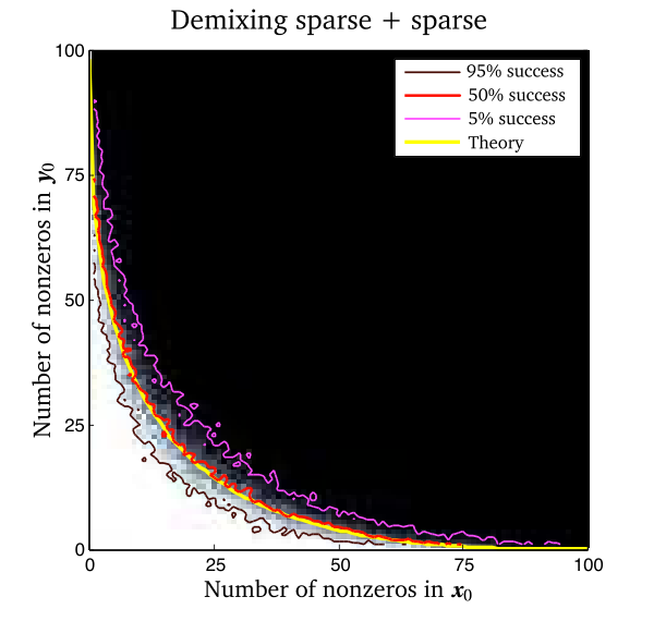
Our numerical work confirms the analysis in Theorem III. Figure 2.6[left] shows when (2.9) can demix a sparse vector from a vector that is sparse in a random basis $\bm{U}$ for $\mathbb{R}^{100}$ . Figure 2.6[right] shows when (2.10) can demix a low-rank matrix from a matrix that is sparse in a random basis $\mathscr{U}$ for $\mathbb{R}^{35\times 35}$ . In each case, the experiment provides an empirical estimate for the probability of success with respect to the randomness in the coherence model. We display the 5%, 50%, and 95% success isoclines, calculated from the data. We also sketch the theoretical phase transition from Theorem III, which occurs when the total statistical dimension of the relevant cones equals the ambient dimension; the statistical dimensions of the descent cones are obtained from the formulas in Sections 4.3 and 4.4. See [MT14b, Sec. 6] for the details of the experimental protocol.

Once again, we see that the theoretical curve of Theorem III coincides almost perfectly with the empirical 50% success isocline. The width of the transition region is $O(\sqrt{d})$ . Although Theorem III does not predict the tapering of the transition in the top-left and bottom-right corners, the discussion in Section 7.1 exposes the underlying reason for this phenomenon.

2.7. Contributions

It takes a substantial amount of argument to establish the existence of phase transitions and to calculate their location for specific problems. Some parts of our paper depend on prior work, but much of the research is new. We conclude this section with a summary of our contributions. Section 10 contains a detailed discussion of the literature; additional citations appear throughout the presentation.

This paper contains foundational research in conic integral geometry:

•

We define the statistical dimension as the mean value of the distribution of intrinsic volumes, and we argue that the statistical dimension canonically extends the linear dimension of a subspace to the class of convex cones. (Definition 2.2 and Section 5.6)
•

We demonstrate that the metric characterization of the statistical dimension coincides with the intrinsic characterization, and we use this connection to establish some properties of the statistical dimension. The statistical dimension is also related to the Gaussian width. (Definition 2.2, Proposition 2.4, Proposition 3.1, Proposition 5.12, and Proposition 10.2)
•

We prove that the distribution of intrinsic volumes of a convex cone concentrates sharply about the statistical dimension of the cone. (Theorem 6.1)
•

The concentration of intrinsic volumes leads to an approximate version of the kinematic formula for cones. This result uses the statistical dimension to bound the probability that a randomly rotated cone shares a ray with a fixed cone. (Theorem I and Theorem 7.1)

Building on this foundation, we establish a number of applied results concerning phase transition phenomena in convex optimization problems with random data:

•

We prove that a regularized linear inverse problem with random measurements must exhibit a phase transition as the number of random measurements increases. The location and width of the transition are controlled by the statistical dimension of a descent cone. Our work confirms and extends the earlier analyses based on polytope angles [Don06a, DT09a, KXAH11, XH12] and those based on Gaussian process theory [RV08, Sto09, OH10, CRPW12]. (Theorem II, Theorem 7.1, and Proposition 9.1)
•

The paper [MT14b] proposes convex programming methods for decomposing a superposition of two structured, randomly oriented vectors into its constituents. We prove that these methods exhibit a phase transition whose properties depend on the total statistical dimension of two descent cones. This work confirms a conjecture [MT14b, Sec. 4.2.2] about the existence of phase transitions in these problems. (Theorem III and Theorem 7.1)
•

The work [AB12] studies cone programs with random affine constraints. Building on this analysis, we show that a cone program with random affine constraints displays a phase transition as the number of constraints increases. We can predict the transition using the statistical dimension of the cone. (Theorem 8.1)
•

Section 4 contains a recipe for estimating the statistical dimension of a descent cone. The approach is based on ideas from [CRPW12, App. C], but we provide the first proof that it delivers accurate estimates. This result rigorously explains why the bounds computed in [Sto09, OH10] closely match observed phase transitions. (Theorem 4.3 and Propositions 4.5 and 4.7)
•

The approximate kinematic formula also delivers information about the probability that a face of a polytope maintains its dimension under a random projection. This argument clarifies the connection between the polytope-angle approach to random linear inverse problems and the approach based on Gaussian process theory. (Section 10.1.1)

As an added bonus, we provide the final ingredient needed to resolve a series of conjectures [DMM09a, DJM13, DGM13] about the coincidence between the minimax risk of denoising and the location of phase transitions in linear inverse problems. Indeed, Oymak & Hassibi [OH13] have recently shown that the minimax risk is equivalent with the statistical dimension of an appropriate cone, and our results prove that the phase transition occurs at precisely this spot. See Section 10.4 for further details.

3. Calculating the statistical dimension

Section 2 demonstrates that the statistical dimension is a fundamental quantity in conic integral geometry. Through the approximate kinematic formula, Theorem I, the statistical dimension drives phase transitions in random linear problems and random demixing problems. A natural question, then, is how we can determine the value of the statistical dimension for a specific cone.

This section explains how to compute the statistical dimension directly for a few basic cones. In Section 3.1, we present some useful properties of the statistical dimension. Sections 3.2–3.5 contain some example calculations, in increasing order of difficulty. See Table 3.1 for a summary. We discuss general descent cones later, in Section 4.

3.1. Basic facts about the statistical dimension

The statistical dimension has a number of valuable properties. These facts provide useful tools for making computations, and they strengthen the analogy between the statistical dimension of a cone and the linear dimension of a subspace.

Proposition 3.1 (Properties of statistical dimension).

Let $C$ be a closed convex cone in $\mathbb{R}^{d}$ . The statistical dimension obeys the following laws.

(1)

Intrinsic formulation. The statistical dimension is defined as

$\delta(C):=\sum_{k=0}^{d}k\,v_{k}(C)$ (3.1)

where $v_{0},\dots,v_{d}$ denote the conic intrinsic volumes. (See Section 5.1.)

(2)

Gaussian formulation. The statistical dimension satisfies

\delta(C)=\operatorname{\mathbb{E}}{}\big[\left\|{\smash{\bm{\Pi}_{C}(\bm{g})}}\right\|^{2}\big]\quad\text{where $\bm{g}\sim\textsc{normal}(\bm{0},\mathbf{I}_{d})$.}

(3.2)

(3)

Spherical formulation. An equivalent expression is

\delta(C)=d\,\operatorname{\mathbb{E}}{}\big[\left\|{\smash{\bm{\Pi}_{C}(\bm{\theta})}}\right\|^{2}\big]\quad\text{where $\bm{\theta}\sim\textsc{uniform}(\mathsf{S}^{d-1})$.}

(3.3)

(4)

Polar formulation. The statistical dimension can be expressed in terms of the polar cone:

$\delta(C)=\operatorname{\mathbb{E}}\big[\dist^{2}(\bm{g},C^{\circ})\big].$ (3.4)

(5)

Mean-squared-width formulation. Another alternative formulation reads

\delta(C)=\operatorname{\mathbb{E}}{}\bigl[\bigl(\sup\nolimits_{\bm{y}\in C\cap\mathsf{B}^{d}}\left\langle{\smash{\bm{y}}},\ {\smash{\bm{g}}}\right\rangle\bigr)^{2}\bigr]\quad\text{where $\bm{g}\sim\textsc{normal}(\bm{0},\mathbf{I}_{d})$.}

(3.5)

(6)

Rotational invariance. The statistical dimension does not depend on the orientation of the cone:

$\delta(\bm{U}C)=\delta(C)\quad\text{for each orthogonal matrix $\bm{U}\in\mathbb{R}^{d\times d}$.}$ (3.6)
(7)

Subspaces. For each subspace $L$ , the statistical dimension satisfies $\delta(L)=\dim(L)$ .
(8)

Complementarity. The sum of the statistical dimension of a cone and that of its polar equals the ambient dimension:

$\delta(C)+\delta(C^{\circ})=d.$ (3.7)

This generalizes the property $\dim(L)+\dim(L^{\perp})=d$ for each subspace $L\subset\mathbb{R}^{d}$ .
(9)

Direct products. For each closed convex cone $K\subset\mathbb{R}^{d}$ ,

$\delta(C\times K)=\delta(C)+\delta(K).$ (3.8)

In particular, the statistical dimension is invariant under embedding:

$\delta\big(C\times\{\bm{0}_{d^{\prime}}\}\big)=\delta(C).$

The relation (3.8) generalizes the rule $\dim(L\times M)=\dim(L)+\dim(M)$ for linear subspaces $L$ and $M$ .
(10)

Monotonicity. For each closed convex cone $K\subset\mathbb{R}^{d}$ , the inclusion $C\subset K$ implies that $\delta(C)\leq\delta(K)$ .

We verify the equivalence of the intrinsic volume formulation (3.1) and the metric formulation (3.2) below in Proposition 5.12. It is possible to establish the remaining facts on the basis of either (3.1) or (3.2). In Appendix B.4, we use the metric characterization (3.2) to prove the rest of the proposition. Many of these elementary results have appeared in [Sto09, CRPW12] in a slightly different form.

Table 3.1. The statistical dimensions of some convex cones.

Cone	Notation	Statistical dimension	Location
The nonnegative orthant	$\mathbb{R}_{+}^{d}$	$\tfrac{1}{2}d$	Sec. 3.2
The second-order cone	$\mathbb{L}^{d+1}$	$\tfrac{1}{2}(d+1)$	Sec. 3.2
Symmetric positive- semidefinite matrices	$\mathbb{S}_{+}^{n\times n}$	$\tfrac{1}{4}n(n+1)$	Sec. 3.2
Descent cone of the $\ell_{\infty}$ norm at an $s$ -saturated vector $\bm{x}$ in $\mathbb{R}^{d}$	$\mathcal{D}(\left\\|{\cdot}\right\\|_{\infty},\bm{x})$	$d-\tfrac{1}{2}s$	Sec. 3.3
Circular cone in $\mathbb{R}^{d}$ of angle $\alpha$	$\Circ_{d}(\alpha)$	$d\sin^{2}(\alpha)+O(1)$	Sec. 3.4
Chambers of finite reflection groups acting on $\mathbb{R}^{d}$	$\begin{array}[]{c}C_{A}\\[2.0pt] C_{BC}\end{array}$	$\begin{array}[]{c}\log(d)+O(1)\\[2.0pt] \tfrac{1}{2}\log(d)+O(1)\end{array}$	Sec. 3.5

3.2. Self-dual cones

We say that a cone $C$ is self-dual when $C^{\circ}=-C$ . Self-dual cones are ubiquitous in the theory and practice of convex optimization. Here are three important examples:

(1)

The nonnegative orthant. The cone $\mathbb{R}_{+}^{d}:=\big\{\bm{x}\in\mathbb{R}^{d}:x_{i}\geq 0\ \text{for $i=1,\dots,d$}\big\}$ is self-dual.
(2)

The second-order cone. The cone $\mathbb{L}^{d+1}:=\big\{(\bm{x},\tau)\in\mathbb{R}^{d+1}:\left\|{\bm{x}}\right\|\leq\tau\big\}$ is self-dual. This example is sometimes called the Lorentz cone or the ice-cream cone.
(3)

Symmetric positive-semidefinite matrices. The cone $\mathbb{S}_{+}^{n\times n}:=\big\{\bm{X}\in\mathbb{R}^{n\times n}_{\text{sym}}:\bm{X}\succcurlyeq\bm{0}\big\}$ is self-dual, where the curly inequality denotes the semidefinite order. Note that the linear space $\mathbb{R}^{n\times n}_{\text{sym}}$ of $n\times n$ symmetric matrices has dimension $\tfrac{1}{2}n(n+1)$ .

For a self-dual cone, the computation of the statistical dimension is particularly simple; cf. [CRPW12, Cor. 3.8]. The first three entries in Table 3.1 follow instantly from this result.

Proposition 3.2 (Self-dual cones).

Let $C$ be a self-dual cone in $\mathbb{R}^{d}$ . The statistical dimension $\delta(C)=\tfrac{1}{2}d$ .

Proof.

Just observe that $\delta(C)=\tfrac{1}{2}\big[\delta(C)+\delta(C^{\circ})\big]=\tfrac{1}{2}d$ . The first identity holds because of the self-dual property of the cone and the rotational invariance (3.6) of statistical dimension. The second equality follows from the complementarity law (3.7). ∎

3.3. Descent cones of the $\ell_{\infty}$ norm

Recall that the $\ell_{\infty}$ norm of a vector $\bm{x}\in\mathbb{R}^{d}$ is defined as

\left\|{\bm{x}}\right\|_{\infty}:=\max_{i=1,\dots,d}\ \left|{x_{i}}\right|.

The descent cones of the $\ell_{\infty}$ norm have a simple form that allows us to calculate their statistical dimensions easily. We have drawn this analysis from [McC13, Sec. 6.2.4]. Variants of this result drive the applications in [DT10a, JFF12]. Section 4 develops a method for studying more general types of descent cones.

Proposition 3.3 (Descent cones of the $\ell_{\infty}$ norm).

Consider an $s$ -saturated vector $\bm{x}\in\mathbb{R}^{d}$ ; that is,

\#\big\{i:\left|{x_{i}}\right|=\left\|{\bm{x}}\right\|_{\infty}\big\}=s\quad\text{where $1\leq s\leq d$.}

Then

\mathcal{D}(\left\|{\cdot}\right\|_{\infty},\bm{x})=d-\tfrac{1}{2}s.

Proof sketch.

The $\ell_{\infty}$ norm is homogeneous and invariant under signed permutation, so we may assume that the $s$ -saturated vector $\bm{x}\in\mathbb{R}^{d}$ takes the form

\bm{x}=(1,\dots,1,x_{s+1},\dots,x_{d})^{T}\quad\text{where $1>x_{s+1}\geq\cdots\geq x_{d}\geq 0$.}

The descent cone of the $\ell_{\infty}$ norm at the vector $\bm{x}$ can be written as

\mathcal{D}(\left\|{\cdot}\right\|_{\infty},\bm{x})=\big(-\mathbb{R}_{+}^{s}\big)\times\mathbb{R}^{d-s}.

We may now calculate the statistical dimension:

\delta\big(\mathcal{D}(\left\|{\cdot}\right\|_{\infty},\bm{x})\big)=\delta\big(\mathbb{R}_{+}^{s}\big)+\delta\big(\mathbb{R}^{d-s}\big)=\tfrac{1}{2}s+(d-s)=d-\tfrac{1}{2}s.

The first identity follows from the direct product law (3.8) and the rotational invariance (3.6) of the statistical dimension. The next relation depends on the rule for subspaces and the calculation of the statistical dimension of the nonnegative orthant from Section 3.2. ∎

3.4. Circular cones

The circular cone $\Circ_{d}(\alpha)$ in $\mathbb{R}^{d}$ with angle $0\leq\alpha\leq\tfrac{\pi}{2}$ is defined as

\Circ_{d}(\alpha):=\big\{\bm{x}\in\mathbb{R}^{d}:x_{1}\geq\left\|{\bm{x}}\right\|\cos(\alpha)\big\}.

In particular, the cone $\Circ_{d}(\tfrac{\pi}{4})$ is isometric to the second-order cone $\mathbb{L}^{d}$ . Circular cones have numerous applications in optimization; we refer the reader to [BV04, Sec. 4], [BTN01, Sec. 3], and [AG03] for details.

We can obtain an accurate expression for the statistical dimension of a circular cone by expressing the spherical formulation (3.3) in spherical coordinates and administering a dose of asymptotic analysis.

Proposition 3.4 (Circular cones).

The statistical dimension of a circular cone satisfies

\delta\big(\Circ_{d}(\alpha)\big)=d\sin^{2}(\alpha)+O(1).

(3.9)

The error term is approximately equal to $\cos(2\alpha)$ . See Figure 4.1[left] for a plot of (3.9).

Turn to Appendix D.1 for the proof, which seems to be novel. Even though the formula in Proposition 3.4 is simple, it already gives an excellent approximation in moderate dimensions. See [MT14a, Sec. 6.3] or [MHWG13] for refinements of Proposition 3.4 that appeared after our work.

Figure 3.1. Normal cone at the vertex of a permutahedron. The signed permutahedron

\mathscr{P}_{\pm}(\bm{x})

generated by [left] the vector

\bm{x}=(3,-1)

and [right] the vector

\bm{x}=(3,-2)

. In each panel, the darker cone is the normal cone

\mathcal{N}(\mathscr{P}_{\pm}(\bm{x}),\bm{x})

, and the lighter cone is its polar. Note that the normal cone does not depend on the generator

\bm{x}

provided that the entries of

\bm{x}

are distinct.

3.5. Normal cones of a permutahedron

We close this section with a more sophisticated example. The (signed) permutahedron generated by a vector $\bm{x}\in\mathbb{R}^{d}$ is the convex hull of all (signed) coordinate permutations of the vector:

	$\displaystyle\mathcal{P}(\bm{x})$	$\displaystyle:=\operatorname{conv}\big\{\sigma(\bm{x}):\text{$\sigma$ a coordinate permutation}\big\}$		(3.10)
	$\displaystyle\mathcal{P}_{\pm}(\bm{x})$	$\displaystyle:=\operatorname{conv}\big\{\sigma_{\pm}(\bm{x}):\text{$\sigma_{\pm}$ a signed coordinate permutation}\big\}.$		(3.11)

A signed permutation permutes the coordinates of a vector and may change the sign of each coordinate. The normal cone $\mathcal{N}(E,\bm{x})$ of a convex set $E\subset\mathbb{R}^{d}$ at a point $\bm{x}\in E$ consists of the outward normals to all hyperplanes that support $E$ at $\bm{x}$ , i.e.,

\mathcal{N}(E,\bm{x}):=\big\{\bm{s}\in\mathbb{R}^{d}:\left\langle{\bm{s}},\ {\smash{\bm{y}}-\bm{x}}\right\rangle\leq 0\quad\text{for all $\bm{y}\in E$}\big\}.

(3.12)

Figure 3.1 displays two signed permutahedra along with the normal cone at a vertex of each one.

We can develop an exact formula for the statistical dimension of the normal cone of a nondegenerate permutahedron. In Section 9, we use this calculation to study a signal processing application proposed in [CRPW12, p. 812].

Proposition 3.5 (Normal cones of permutahedra).

Suppose that $\bm{x}$ is a vector in $\mathbb{R}^{d}$ with distinct entries. The statistical dimension of the normal cone at a vertex of the (signed) permutahedron generated by $\bm{x}$ satisfies

\delta\big(\mathcal{N}(\mathcal{P}(\bm{x}),\bm{x})\big)=\mathrm{H}_{d}\quad\text{and}\quad\delta\big(\mathcal{N}(\mathcal{P}_{\pm}(\bm{x}),\bm{x})\big)=\tfrac{1}{2}\mathrm{H}_{d},

where $\mathrm{H}_{d}:=\sum_{i=1}^{d}i^{-1}$ is the $d$ th harmonic number.

The proof of Proposition 3.5 appears in Appendix D.4. The argument relies on the intrinsic formulation (3.1) of the statistical dimension, and it illustrates some deep connections between conic geometry and classical combinatorics.

4. The statistical dimension of a descent cone

Theorems II and III allow us to locate the phase transition for a class of convex optimization problems with random data. To apply these results, however, we must be able to compute the statistical dimension for the descent cone of a convex function. In this section, we describe a recipe that delivers an accurate estimate for the statistical dimension of a descent cone.

In Section 4.1, we explain how to obtain an upper bound for the statistical dimension of a descent cone. Section 4.2 provides an error estimate for this method. In Sections 4.3 and 4.4, we apply these ideas to study the descent cones of the $\ell_{1}$ norm and the Schatten 1-norm.

4.1. A recipe for the statistical dimension of a descent cone

There is an elegant way to obtain an upper bound for the statistical dimension of a descent cone of a convex function. Recall that the subdifferential $\partial f(\bm{x})$ of a proper convex function $f:\mathbb{R}^{d}\to\overline{\mathbb{R}}$ at a point $\bm{x}\in\mathbb{R}^{d}$ is the closed convex set

\partial f(\bm{x}):=\big\{\bm{s}\in\mathbb{R}^{d}:f(\bm{y})\geq f(\bm{x})+\left\langle{\bm{s}},\ {\smash{\bm{y}}-\bm{x}}\right\rangle\text{ for all $\bm{y}\in\mathbb{R}^{d}$}\big\}.

There is a classical duality between descent cones and subdifferentials [Roc70, Chap. 23]. As a consequence, we can convert questions about the statistical dimension of a descent cone into questions about the subdifferential.

Proposition 4.1 (The statistical dimension of a descent cone).

Let $f:\mathbb{R}^{d}\to\overline{\mathbb{R}}$ be a proper convex function, and let $\bm{x}\in\mathbb{R}^{d}$ . Assume that the subdifferential $\partial f(\bm{x})$ is nonempty, compact, and does not contain the origin. Define the function

J(\tau):=J(\tau;\ \partial f(\bm{x})):=\operatorname{\mathbb{E}}\big[\dist^{2}\big(\bm{g},\tau\cdot\partial f(\bm{x})\big)\big]\quad\text{for $\tau\geq 0$}

(4.1)

where $\bm{g}\sim\textsc{normal}(\bm{0},\mathbf{I})$ . We have the upper bound

\delta\big(\mathcal{D}(f,\bm{x})\big)\leq\inf_{\tau\geq 0}\ J(\tau).

(4.2)

Furthermore, the function $J$ is strictly convex, continuous at $\tau=0$ , and differentiable for $\tau\geq 0$ . It achieves its minimum at a unique point.

Proof.

The inequality (4.2) generalizes some specific arguments from [CRPW12, App. C], and it is easy to establish. We use the polarity relation (3.4) to compute the statistical dimension:

\delta\big(\mathcal{D}(f,\bm{x})\big)=\delta\big(\mathcal{D}(f,\bm{x})^{\circ\circ}\big)=\operatorname{\mathbb{E}}\big[\dist^{2}\big(\bm{g},{}\mathcal{D}(f,\bm{x})^{\circ}\big)\big]=\operatorname{\mathbb{E}}\left[\dist^{2}\left(\bm{g},\bigcup_{\tau\geq 0}\tau\cdot\partial f(\bm{x})\right)\right]=\operatorname{\mathbb{E}}{}\bigg[\inf_{\tau\geq 0}\ \dist^{2}\big(\bm{g},\tau\cdot\partial f(\bm{x})\big)\bigg].

Indeed, the statistical dimension of the descent cone equals the statistical dimension of its closure, which can be expressed as a double polar. The second identity uses (3.4) and the fact that polarity is an involution on closed convex cones. The third identity follows from the fact that, under our technical assumptions, the polar of the descent cone is the cone generated by the subdifferential [Roc70, Cor. 23.7.1]; see Appendix B.1 for details. The last identity holds because the distance to a union is the infimal distance to any one of its members. To reach (4.2), we pass the expectation through the infimum.

The analytic properties of the function $J$ are new, and they demand substantial effort. Lemma C.2 in Appendix C.1 contains the proof of the remaining claims. ∎

Proposition 4.1 suggests a method for studying the statistical dimension of a descent cone: Minimize the function $J$ by setting its derivative to zero. We formalize this approach in Recipe 4.1. In Section 4.3 and 4.4, we discuss some examples where this recipe is provably effective.

Remark 4.2 (Prior work).

Rudelson & Vershynin [RV08, Sec. 4] established a bound for the Gaussian width of the descent cone of the $\ell_{1}$ norm at a sparse vector using a geometric argument. Stojnic [Sto09] obtained a substantial refinement of this estimate using linear programming duality. Oymak & Hassibi [OH10] developed a related method to study the descent cone of the Schatten 1-norm at a low-rank matrix. The paper [CRPW12, App. C] clarifies the calculations of Stojnic and Oymak & Hassibi using geometric polarity arguments. The result (4.2) extends the latter approach to a general convex function.

4.2. An error estimate for the descent cone recipe

The papers [Sto09, OH10] contain computational evidence that the ideas behind Recipe 4.1 lead to accurate upper bounds in some special cases. Among the major contributions of this paper is an error estimate that explains why the descent cone recipe works so well. This result is an essential ingredient in our method for locating the phase transition of a random convex program. Indeed, we need this theorem to ensure that we can calculate the statistical dimension of a descent cone correctly.

Theorem 4.3 (Error bound for descent cone recipe).

Let $f$ be a norm on $\mathbb{R}^{d}$ , and fix a nonzero point $\bm{x}\in\mathbb{R}^{d}$ . Then

0\leq\bigg(\inf_{\tau\geq 0}\ J(\tau;\ \partial f(\bm{x}))\bigg)-\delta\big(\mathcal{D}(f,\bm{x})\big)\leq\frac{2\,\sup\big\{\left\|{\bm{s}}\right\|:\bm{s}\in\partial f(\bm{x})\big\}}{f(\bm{x}/\left\|{\bm{x}}\right\|)},

(4.3)

where the function $J$ is defined in (4.1).

The proof of Theorem 4.3 is technical in nature, so we defer the details to Appendix C.2. The application of this result requires some care because many different vectors $\bm{x}$ can generate the same subdifferential $\partial f(\bm{x})$ and hence the same descent cone $\mathcal{D}(f,\bm{x})$ . From this class of vectors, we ought to select one that maximizes the value $f(\bm{x}/\left\|{\bm{x}}\right\|)$ .

Remark 4.4 (Related work).

In an independent paper that appeared shortly after this work was released, Foygel & Mackey [FM14] developed another error bound for the descent cone recipe. These two results operate under different assumptions, and the two bounds are effective in different regimes. It remains an open question to find an optimal error estimate for Recipe 4.1.

Recipe 4.1: The statistical dimension of a descent cone.

Assume that $f:\mathbb{R}^{d}\to\overline{\mathbb{R}}$ is a proper convex function and $\bm{x}\in\mathbb{R}^{d}$ Assume that the subdifferential $\partial f(\bm{x})$ is nonempty, compact, and does not contain the origin (1) Identify the subdifferential $S=\partial f(\bm{x})$ . (2) For each $\tau\geq 0$ , compute $J(\tau)=\operatorname{\mathbb{E}}\big[\dist^{2}(\bm{g},\tau S)\big]$ . (3) Find the unique solution, if it exists, to the stationary equation $J^{\prime}(\tau)=0$ . (4) If the stationary equation has a solution $\tau_{\star}$ , then $\delta\big(\mathcal{D}(f,\bm{x})\big)\leq J(\tau_{\star})$ . (5) Otherwise, the bound is vacuous: $\delta\big(\mathcal{D}(f,\bm{x})\big)\leq J(0)=d$ .

4.3. Descent cones of the $\ell_{1}$ norm

When we wish to solve an inverse problem with a sparse unknown, we often use the $\ell_{1}$ norm as a regularizer; cf. (2.5), (2.9), and (2.10). Our next result summarizes the calculations required to obtain the statistical dimension of the descent cone of the $\ell_{1}$ norm at a sparse vector. When we combine this proposition with Theorems II and III, we obtain the exact location of the phase transition for $\ell_{1}$ regularized inverse problems whose dimension is large.

Proposition 4.5 (Descent cones of the $\ell_{1}$ norm).

Let $\bm{x}$ be a vector in $\mathbb{R}^{d}$ with $s$ nonzero entries. Then the normalized statistical dimension of the descent cone of the $\ell_{1}$ norm at $\bm{x}$ satisfies the bounds

\psi(s/d)-\frac{2}{\sqrt{sd}}\leq\frac{\delta\big(\mathcal{D}(\left\|{\cdot}\right\|_{1},\bm{x})\big)}{d}\leq\psi(s/d).

(4.4)

The function $\psi:[0,1]\to[0,1]$ is defined as

\psi(\rho):=\inf_{\tau\geq 0}\ \left\{\rho(1+\tau^{2})+(1-\rho)\int_{\tau}^{\infty}(u-\tau)^{2}\cdot\varphi(u)\,\mathrm{d}{u}\right\}.

(4.5)

The integral kernel $\varphi(u):=\sqrt{2/\pi}\,\mathrm{e}^{-u^{2}/2}$ is a probability density supported on $[0,\infty)$ . The infimum in (4.5) is achieved for the unique positive $\tau$ that solves the stationary equation

\int_{\tau}^{\infty}\left(\frac{u}{\tau}-1\right)\cdot\varphi(u)\,\mathrm{d}{u}=\frac{\rho}{1-\rho}.

(4.6)

See Figure 4.1[center] for a plot of the function (4.5).

Proposition 4.5 is a direct consequence of Recipe 4.1 and the error bound in Theorem 4.3. See Appendix D.2 for details of the proof; Appendix A.2 explains the numerical aspects.

Let us emphasize the following consequences of Proposition 4.5. When the number $s$ of nonzeros in the vector $\bm{x}$ is proportional to the ambient dimension $d$ , the error in the statistical dimension calculation (4.4) is vanishingly small relative to the ambient dimension. When $\bm{x}$ is sparser, it is more appropriate to compare the error with the statistical dimension itself. Thus,

0\leq\frac{\big(d\cdot\psi(s/d)\big)-\delta\big(\mathcal{D}(\left\|{\cdot}\right\|_{1},\bm{x})\big)}{\delta\big(\mathcal{D}(\left\|{\cdot}\right\|_{1},\bm{x})\big)}\leq\frac{2}{\sqrt{\delta\big(\mathcal{D}(\left\|{\cdot}\right\|_{1},\bm{x})\big)}}\quad\text{when $s\geq\sqrt{d}+1$.}

We have used the observation that $\delta\big(\mathcal{D}(\left\|{\cdot}\right\|_{1},\bm{x})\big)\geq s-1$ , which holds because $\mathcal{D}(\left\|{\cdot}\right\|_{1},\bm{x})$ contains the $(s-1)$ -dimensional subspace parallel with the minimal face of the $\ell_{1}$ ball containing $\bm{x}$ .

Remark 4.6 (Prior work).

Except for the first inequality in (4.4), the calculations and the resulting formulas in Proposition 4.5 are not substantially novel. Most of the existing analysis concerns the phase transition in compressed sensing, i.e., the $\ell_{1}$ minimization problem (2.5) with Gaussian measurements. In this setting, Donoho [Don06b] and Donoho & Tanner [DT09a] obtained an asymptotic upper bound, equivalent to the upper bound in (4.4), from polytope angle calculations. Stojnic [Sto09] established the same asymptotic upper bound using a precursor of Recipe 4.1; see also [CRPW12, App. C]. In addition, there are some heuristic arguments, based on ideas from statistical physics, that lead to the same result, cf. [DMM09a] and [DMM09b, Sec. 17]. Very recently, Bayati et al. [BLM13a] have shown that, in the asymptotic setting, the compressed sensing problem undergoes a phase transition at the location predicted by (4.4).

Figure 4.1. Asymptotic statistical dimension computations. In each panel, we take the dimensional parameters to infinity. [left] Circular cones. The plot shows the normalized statistical dimension

\delta(\cdot)/d

of the circular cone

\Circ_{d}(\alpha)

. [center]

\ell_{1}

descent cones. The curve traces the normalized statistical dimension

\delta(\cdot)/d

of the descent cone of the

\ell_{1}

norm on

\mathbb{R}^{d}

at a vector with

\lfloor\rho d\rfloor

nonzero entries. [right] Schatten 1-norm descent cones. The normalized statistical dimension

\delta(\cdot)/(mn)

of the descent cone of the

S_{1}

norm on

\mathbb{R}^{m\times n}

at a matrix with rank

\lfloor\rho m\rfloor

for several fixed aspect ratios

\nu=m/n

. As the aspect ratio

\nu\to 0

, the limiting curve is

\rho\mapsto 2\rho-\rho^{2}

4.4. Descent cones of the Schatten 1-norm

When we wish to solve an inverse problem whose unknown is a low-rank matrix, we often use the Schatten 1-norm $S_{1}$ as a regularizer, as in (2.6) and (2.10). The following result gives an asymptotically exact expression for the statistical dimension of the descent cone of the $S_{1}$ norm at a low-rank matrix. Together with Theorems II and III, this proposition allows us to identify the exact location of the phase transition for $S_{1}$ regularized inverse problems as the ambient dimension goes to infinity.

Proposition 4.7 (Descent cones of the $S_{1}$ norm).

Consider a sequence $\{\bm{X}(r,m,n)\}$ of matrices where $\bm{X}(r,m,n)$ has rank $r$ and dimension $m\times n$ with $m\leq n$ . Suppose that $r,m,n\to\infty$ with limiting ratios $r/m\to\rho\in(0,1)$ and $m/n\to\nu\in(0,1]$ . Then

\frac{\delta\big(\mathcal{D}\big(\left\|{\cdot}\right\|_{S_{1}},\bm{X}(r,m,n)\big)\big)}{mn}\to\psi(\rho,\nu).

(4.7)

The function $\psi:[0,1]\times[0,1]\to[0,1]$ is defined as

\psi(\rho,\nu):=\inf_{\tau\geq 0}\ \left\{\rho\nu+(1-\rho\nu)\left[\rho\big(1+\tau^{2}\big)+(1-\rho)\int_{a_{-}\vee\tau}^{a_{+}}(u-\tau)^{2}\cdot\varphi_{y}(u)\,\mathrm{d}{u}\right]\right\}.

(4.8)

The quantity $y:=(\nu-\rho\nu)/(1-\rho\nu)$ , and the limits of the integral are $a_{\pm}:=1\pm\sqrt{y}$ . The integral kernel $\varphi_{y}$ is a probability density supported on $[a_{-},a_{+}]$ :

\varphi_{y}(u):=\frac{1}{\pi yu}\sqrt{(u^{2}-a_{-}^{2})(a_{+}^{2}-u^{2})}\quad\text{for $u\in[a_{-},a_{+}]$.}

The optimal value of $\tau$ in (4.8) satisfies the stationary equation

\int_{a_{-}\vee\tau}^{a_{+}}\left(\frac{u}{\tau}-1\right)\cdot\varphi_{y}(u)\,\mathrm{d}{u}=\frac{\rho}{1-\rho}.

(4.9)

See Figure 4.1[right] for a visualization of the curve (4.8) as function of $\rho$ for several choices of $\nu$ . The operator $\vee$ returns the maximum of two numbers.

See Appendix D.3 for a proof of Proposition 4.7. Appendix A.2 contains details of the numerical calculation.

Remark 4.8 (Prior work).

The literature contains several papers that, in effect, contain loose upper bounds for the statistical dimension of the descent cones of the Schatten 1-norm [RXH11, OKH11]. We single out the work [OH10] of Oymak & Hassibi, which identifies an empirically sharp upper bound via a laborious argument. The approach here is more in the spirit of the weak upper bound in [CRPW12, App. C], but our argument leads to the asymptotically correct estimate.

5. Conic integral geometry and the statistical dimension

To prove that the statistical dimension controls the location of phase transitions in random convex optimization problems, we rely on methods from conic integral geometry, the field of mathematics concerned with geometric properties of convex cones that remain invariant under rotations, reflections, and embeddings. Here are some of the guiding questions in this area:

•

What is the probability that a random unit vector lies at most a specified distance from a fixed cone?
•

What is the probability that a randomly rotated cone shares a ray with a fixed cone?

The theory of conic integral geometry offers beautiful and precise answers to these questions, phrased in terms of a set of geometric invariants called conic intrinsic volumes.

In Section 5.1, we formally introduce the intrinsic volumes of a cone and we compute the intrinsic volumes of some basic cones. We state the key facts about intrinsic volumes in Section 5.2. Sections 5.3 and 5.4 contain more advanced formulas from conic integral geometry, which are essential tools in our approach to phase transitions. In Section 5.5, we establish the equivalence of the two characterizations of the statistical dimension, given in Definition 2.2 and Proposition 2.4. Section 5.6 explains why the statistical dimension is canonical.

The material in this section is adapted from the book [SW08, Sec. 6.5] and the dissertation [Ame11]. The foundational research in this area is due to Santaló [San76, Part IV]. Modern treatments depend on the work of Glasauer [Gla95, Gla96]. In these sources, the theory is presented in terms of spherical geometry, rather than in terms of conical geometry. As noted in [AB12], the two approaches are equivalent, but the conic viewpoint provides simpler formulas and has other benefits that are revealed by deeper structural investigations.

5.1. Conic intrinsic volumes

We begin with the definition of the intrinsic volumes of a convex cone. Recall that a cone is polyhedral if it can be written as the intersection of a finite number of halfspaces. Polyhedral cones are automatically closed and convex.

Definition 5.1 (Intrinsic volumes: Polyhedral case).

Let $C$ be a polyhedral cone in $\mathbb{R}^{d}$ . For each $k=0,1,2,\dots,d$ , the $k$ th (conic) intrinsic volume $v_{k}(C)$ is given by

v_{k}(C):=\mathbb{P}\big\{\text{$\bm{\Pi}_{C}(\bm{g})$ lies in the relative interior of a $k$-dimensional face of $C$}\big\}.

As usual, $\bm{g}$ is a standard normal vector in $\mathbb{R}^{d}$ . See Figure 5.1 for an illustration.

Figure 5.1. The intrinsic volumes of a convex cone in two dimensions. The closed convex cone

C\subset\mathbb{R}^{2}

has four faces: one two-dimensional face (dark shading), two one-dimensional faces (the boundary rays), and one zero-dimensional face (the origin). The projection

\bm{\Pi}_{C}(\bm{g})

of a standard normal vector

\bm{g}

onto

K

lies in the two-dimensional face when

\bm{g}

is in the dark region, on a one-dimensional face when

\bm{g}

is in the white region, and in the zero-dimensional face when

\bm{g}

is in the light region. Each intrinsic volume of the cone

C

can be expressed in terms of the solid angle

\alpha

measured in radians:

v_{2}(C)=\alpha/(2\pi)

and

v_{1}(C)=1/2

and

v_{0}(C)=(\pi-\alpha)/(2\pi)

For a polyhedral cone, it is clear that the sequence of intrinsic volumes forms a probability distribution on $\{0,1,2,\dots,d\}$ . The definition also delivers insight about several fundamental examples.

Example 5.2 (Linear subspaces).

Let $L_{j}$ be a $j$ -dimensional subspace in $\mathbb{R}^{d}$ . Then $L_{j}$ is a polyhedral cone with precisely one face, so the map $\bm{\Pi}_{L_{j}}$ projects every point onto this $j$ -dimensional face. Thus,

v_{k}(L_{j})=\begin{cases}1,&k=j\\ 0,&k\neq j\end{cases}\quad\text{for $k=0,1,2,\dots,d$.}

Apply the intrinsic formulation (3.1) of the statistical dimension to confirm that $\delta(L_{j})=j$ .

Example 5.3 (The nonnegative orthant).

The nonnegative orthant $\mathbb{R}_{+}^{d}$ is a polyhedral cone. The projection $\bm{\Pi}_{\mathbb{R}_{+}^{d}}(\bm{g})$ lies in the relative interior of a $k$ -dimensional face of the orthant if and only if exactly $k$ coordinates of $\bm{g}$ are positive. Each coordinate of $\bm{g}$ is positive with probability one-half and negative with probability one-half, and the coordinates are independent. Therefore, the intrinsic volumes of the orthant are given by

v_{k}\big(\mathbb{R}_{+}^{d}\big)=2^{-d}{d\choose k}\quad\text{for $k=0,1,2,\dots,d$.}

In other words, the intrinsic volumes coincide with the probability density of a $\textsc{Binomial}(d,\tfrac{1}{2})$ random variable. Apply the intrinsic formulation (3.1) of the statistical dimension to confirm that $\delta\big(\mathbb{R}_{+}^{d}\big)=\tfrac{1}{2}d$ .

Let us explain briefly how to extend the definition of conic intrinsic volumes to the general case. We can equip the family of closed convex cones in $\mathbb{R}^{d}$ with the conic Hausdorff metric²² 2 The conic Hausdorff metric is obtained by identifying each closed convex cone $C\subset\mathbb{R}^{d}$ with the spherical convex set $C\cap\mathsf{S}^{d-1}$ . Then we invoke the familiar construction of the Hausdorff metric on the sphere. to form a compact metric space. The polyhedral cones are dense in this metric space, and the conic intrinsic volumes are continuous with respect to the metric. Therefore, we may define the intrinsic volumes of a general closed convex cone by approximation.

Definition 5.4 (Intrinsic volumes: General case).

Let $C$ be a closed convex cone in $\mathbb{R}^{d}$ , and let $\{C_{i}:i=1,2,3,\dots\}\subset\mathbb{R}^{d}$ be a sequence of polyhedral cones that converges to $C$ in the conic Hausdorff metric. For each $k=0,1,2,\dots,d$ , the $k$ th (conic) intrinsic volume $v_{k}(C)$ is given by the limit

v_{k}(C):=\lim_{i\to\infty}v_{k}(C_{i}).

It can be shown that this limit does not depend on the approximating sequence.

Let us warn the reader that the projection formula in Definition 5.1 breaks down for a general closed convex cone because the limiting process does not preserve facial structure. To learn more about the construction behind Definition 5.4, see the book [SW08, Sec. 6.5], the thesis [Ame11], or the paper [MT14a]. The spherical Steiner formula, Fact 5.7, provides an alternative geometric interpretation of the intrinsic volumes.

5.2. Properties of conic intrinsic volumes

The intrinsic volumes of a closed convex cone satisfy a number of important relationships that we outline here.

Fact 5.5 (Properties of intrinsic volumes).

Let $C$ be a closed convex cone in $\mathbb{R}^{d}$ . The intrinsic volumes of the cone obey the following laws.

(1)

Distribution. The intrinsic volumes describe a probability distribution on $\{0,1,\dots,d\}$ :

$\sum_{k=0}^{d}v_{k}(C)=1\quad\text{and}\quad v_{k}(C)\geq 0\quad\text{for $k=0,1,2,\dots,d$.}$ (5.1)
(2)

Polarity. The intrinsic volumes reverse under polarity:

$v_{k}(C)=v_{d-k}(C^{\circ})\quad\text{for $k=0,1,2,\dots,d$.}$ (5.2)

(3)

Gauss–Bonnet formula. When $C$ is not a subspace,

\sum_{\begin{subarray}{c}k=0\\ \text{$k$ even}\end{subarray}}^{d}v_{k}(C)=\sum_{\begin{subarray}{c}k=1\\ \text{$k$ odd}\end{subarray}}^{d}v_{k}(C)=\frac{1}{2}.

(5.3)

(4)

Direct products. For each convex cone $K\subset\mathbb{R}^{d^{\prime}}$ ,

$v_{k}(C\times K)=\sum_{i+j=k}v_{i}(C)\cdot v_{j}(K)\quad\text{for $k=0,1,2,\dots,d+d^{\prime}$.}$ (5.4)

The facts (5.1), (5.2), and (5.3) are drawn from [SW08, Sec. 6.5]. See [Ame11, Prop. 4.4.13] or [MT14a, Cor. 5.1] for a proof of the product rule (5.4).

5.3. The spherical Steiner formula

We continue with a selection of more sophisticated results from conic integral geometry. These formulas provide detailed answers, expressed in terms of conic intrinsic volumes, to the geometric questions posed at the beginning of Section 5. To state the first result, we introduce a family of geometric functions.

Definition 5.6 (Tropic functions).

Let $L_{k}$ be a $k$ -dimensional subspace of $\mathbb{R}^{d}$ . Define

I_{k}^{d}(\varepsilon):=\mathbb{P}\big\{\left\|{\smash{\bm{\Pi}_{L_{k}}(\bm{\theta})}}\right\|^{2}\geq\varepsilon\big\}\quad\text{for $\varepsilon\in[0,1]$,}

(5.5)

where $\bm{\theta}$ is uniformly distributed on the unit sphere in $\mathbb{R}^{d}$ .

Basic geometric reasoning reveals that $I_{k}^{d}(\varepsilon)$ is the proportion of points on the sphere $\mathsf{S}^{d-1}$ that lie within an angle $\arccos(\sqrt{\varepsilon})$ of the subspace $L_{k}$ . Our terminology derives from the approximate geographical fact that the tropics lie within a fixed angle ( $23^{\circ}\,26^{\prime}$ ) of the equator; the usual term regularized incomplete beta function is longer and less evocative.

The core fact in conic integral geometry is the spherical Steiner formula [Hot39, Wey39, Her43, All48, San50], which describes the fraction of points on the sphere that lie at most a fixed angle from a closed convex cone.

Fact 5.7 (Spherical Steiner formula).

Let $C$ be a closed convex cone in $\mathbb{R}^{d}$ . For each $\varepsilon\in[0,1]$ ,

\mathbb{P}\big\{\left\|{\smash{\bm{\Pi}_{C}(\bm{\theta})}}\right\|^{2}\geq\varepsilon\big\}=\sum_{k=0}^{d}v_{k}(C)\,I_{k}^{d}(\varepsilon).

(5.6)

The spherical Steiner formula often serves as the definition of conic intrinsic volumes. The formula (5.6) can also be derived from the definition here. For a proof of Fact 5.7 in the spirit of this work, see [SW08, Thm. 6.5.1] or [MT14a, Prop. 3.4].

5.4. The conic kinematic formula

Next, we present another major result from the theory of conic integral geometry. This statement involves partial sums of the intrinsic volumes.

Definition 5.8 (Tail functionals).

Let $C$ be a closed convex cone in $\mathbb{R}^{d}$ . For each $k=0,1,2,\dots,d$ , the $k$ th tail functional is given by

	$\displaystyle t_{k}(C)$	$\displaystyle:=v_{k}(C)+v_{k+1}(C)+\dots=\sum_{\hskip 8.19447ptj=k\hskip 8.19447pt}^{d}v_{j}(C).$	(5.7)
The $k$ th half-tail functional is defined as
	$\displaystyle h_{k}(C)$	$\displaystyle:=v_{k}(C)+v_{k+2}(C)+\dots=\sum_{\begin{subarray}{c}j=k\\ \text{$j-k$ even}\end{subarray}}^{d}v_{j}(C).$	(5.8)

The two types of tail functionals are related through the following interlacing inequality.

Proposition 5.9 (Interlacing).

For each closed convex cone $C$ in $\mathbb{R}^{d}$ that is not a linear subspace,

2\,h_{k}(C)\geq t_{k}(C)\geq 2\,h_{k+1}(C)\quad\text{for each $k=0,1,2,\dots,d-1$.}

We establish Proposition 5.9 in Appendix E.

With this notation, we can present a modern formulation of the conic kinematic formula, which provides an exact expression for the probability that a randomly oriented convex cone has a nontrivial intersection with a fixed convex cone.

Fact 5.10 (Conic kinematic formula).

Let $C$ and $K$ be closed convex cones in $\mathbb{R}^{d}$ , and assume that $C$ is not a subspace. Then

	$\displaystyle\mathbb{P}\big\{C\cap\bm{Q}K\neq\{\bm{0}\}\big\}$	$\displaystyle=2\,h_{d+1}(C\times K).$	(5.9)
For a linear subspace $L_{d-m}$ in $\mathbb{R}^{d}$ with dimension $d-m$ , this expression reduces to the Crofton formula
	$\displaystyle\mathbb{P}\big\{C\cap\bm{Q}L_{d-m}\neq\{\bm{0}\}\big\}$	$\displaystyle=2\,h_{m+1}(C).$	(5.10)

The compact notation here disguises the equivalence between (5.9) and Fact 2.1. To verify this point, expand the half-tail functional using (5.8) and apply the direct product rule (3.8). See [SW08, p. 261] for a proof of Fact 5.10.

Remark 5.11 (Extended kinematic formula).

By induction, the kinematic formula generalizes to a family $\{C,K_{1},\dots,K_{r}\}$ of closed convex cones in $\mathbb{R}^{d}$ . If $C$ is not a subspace, then

\mathbb{P}\big\{C\cap\bm{Q}_{1}K_{1}\cap\dots\cap\bm{Q}_{r}K_{r}\neq\{\bm{0}\}\big\}=2\,h_{rd+1}(C\times K_{1}\times\dots\times K_{r}).

(5.11)

Each matrix $\bm{Q}_{i}\in\mathbb{R}^{n\times n}$ is a random orthogonal basis, chosen independently from the others. This result can be used to analyze demixing problems with more than two constituents. See the follow-up work [MT13] for details.

5.5. Characterizations of the statistical dimension

In Section 2, we presented two different ways of thinking about the statistical dimension. Definition 2.2, offers an intrinsic characterization in terms of the conic intrinsic volumes, and it links the statistical dimension to the theory of conic integral geometry. Proposition 2.4 provides a metric characterization that leads to powerful tools for calculating the statistical dimension for specific cones. The following result applies the spherical Steiner formula to verify that the two formulations coincide.

Proposition 5.12 (Statistical dimension: Equivalent characterizations).

For each closed convex cone $C$ in $\mathbb{R}^{d}$ ,

\delta(C)=\operatorname{\mathbb{E}}\big[\left\|{\smash{\bm{\Pi}_{C}(\bm{g})}}\right\|^{2}\big]=\sum_{k=0}^{d}k\,v_{k}(C).

Proof.

The Gaussian formulation (3.2) and the spherical formulation (3.3) of statistical dimension coincide, so

\operatorname{\mathbb{E}}\big[\left\|{\smash{\bm{\Pi}_{C}(\bm{g})}}\right\|^{2}\big]=d\,\operatorname{\mathbb{E}}\big[\left\|{\smash{\bm{\Pi}_{C}(\bm{\theta})}}\right\|^{2}\big]=d\int_{0}^{1}\mathbb{P}\big\{\left\|{\smash{\bm{\Pi}_{C}(\bm{\theta})}}\right\|^{2}\geq\varepsilon\big\}\,\mathrm{d}{\varepsilon}.

We have used integration by parts to express the expectation as an integral of tail probabilities. The Steiner formula (5.6) and the definition (5.5) of the tropic function allow us to write the probability as a sum:

\operatorname{\mathbb{E}}\big[\left\|{\smash{\bm{\Pi}_{C}(\bm{g})}}\right\|^{2}\big]=d\sum_{k=0}^{d}v_{k}(C)\int_{0}^{1}\mathbb{P}\big\{\left\|{\smash{\bm{\Pi}_{L_{k}}(\bm{\theta})}}\right\|^{2}\geq\varepsilon\big\}\,\mathrm{d}{\varepsilon}=\sum_{k=0}^{d}v_{k}(C)\,\big(d\,\operatorname{\mathbb{E}}\big[\left\|{\smash{\bm{\Pi}_{L_{k}}(\bm{\theta})}}\right\|^{2}\big]\big)=\sum_{k=0}^{d}k\,v_{k}(C).

where $L_{k}$ is an arbitrary $k$ -dimensional subspace. The last identity follows from elementary geometric reasoning. ∎

5.6. The statistical dimension is canonical

The intrinsic characterization of the statistical dimension, Definition 2.2, has a significant consequence from the point of view of integral geometry. We summarize the ideas for the benefit of geometers; other readers may prefer to skip this material.

Let $\mathscr{C}_{d}$ denote the family of closed convex cones in $\mathbb{R}^{d}$ , equipped with the conic Hausdorff metric to form a compact metric space. A geometric functional $v:\mathscr{C}_{d}\to\mathbb{R}$ is called a continuous, rotation-invariant valuation if it satisfies the properties

(1)

Valuation I. For the trivial cone, $v(\{\bm{0}\})=0$ .
(2)

Valuation II. If $C,K\in\mathscr{C}_{d}$ and $C\cup K\in\mathscr{C}_{d}$ , then $v(C\cup K)+v(C\cap K)=v(C)+v(K)$ .
(3)

Rotation invariance. For each $C\in\mathscr{C}_{d}$ , we have $v(\bm{U}C)=v(C)$ for each orthogonal matrix $\bm{U}\in\mathbb{R}^{d\times d}$ .
(4)

Continuity. If $C_{i}\to C$ in $\mathscr{C}_{d}$ , then $\lim_{i\to\infty}v(C_{i})\to v(C)$ .

Continuous, rotation-invariant valuations are natural geometric measures defined on convex cones. Many of the valuations that arise in conic geometry are also localizable, which is a subtle technical property [SW08, p. 254].

In particular, each intrinsic volume $v_{k}$ is a continuous, rotation-invariant, localizable valuation on the set of closed convex cones. It follows from the intrinsic formulation (3.1) that the statistical dimension inherits these technical properties. It is known that each continuous, rotation-invariant, and localizable valuation on $\mathscr{C}_{d}$ is determined by the values it takes on linear subspaces; see [Gla95, Satz 4.2.2], [Gla96, Thm. 5], or [SW08, Thm. 6.5.4]. Therefore,

The statistical dimension $\delta$ is the unique continuous, rotation-invariant, localizable valuation on the set $\mathscr{C}_{d}$ of closed convex cones that satisfies $\delta(L)=\dim(L)$ for each subspace $L$ .

In other words, the statistical dimension canonically extends the linear dimension to the class of closed convex cones.

The long-standing spherical Hadwiger conjecture states that the condition of localizability is unnecessary here. More precisely, the conjecture posits that every continuous and rotation-invariant valuation on the set of closed convex cones can be expressed as a linear combination of the conic intrinsic volumes. For a discussion of the spherical Hadwiger conjecture, see the works [McM93, p. 976], [KR97, Sec. 11.5], and [SW08, p. 263]. The conjecture currently stands open for $d\geq 4$ .

6. Intrinsic volumes concentrate at the statistical dimension

The main technical result in this paper describes a new property of conic intrinsic volumes: The intrinsic volumes of a closed convex cone concentrate near the statistical dimension of the cone on a scale determined by the statistical dimension. This phenomenon is depicted in Figure 2.2.

Theorem 6.1 (Concentration of intrinsic volumes).

Let $C$ be a closed convex cone. Define the transition width

\omega(C):=\sqrt{\delta(C)\wedge\delta(C^{\circ})},

and introduce the function

p_{C}(\lambda):=4\exp\left(\frac{-\lambda^{2}/8}{\omega^{2}(C)+\lambda}\right)\quad\text{for $\lambda\geq 0$.}

(6.1)

Then

	$\displaystyle k_{-}\leq\delta(C)-\lambda+1$	$\displaystyle\quad\Longrightarrow\quad t_{k_{-}}(C)\geq 1-p_{C}(\lambda);$		(6.2)
	$\displaystyle k_{+}\geq\delta(C)+\lambda\phantom{\ +1}$	$\displaystyle\quad\Longrightarrow\quad t_{k_{+}}(C)\leq\phantom{1-\ }p_{C}(\lambda).$		(6.3)

The tail functional $t_{k}$ is defined in (5.7). The operator $\wedge$ returns the minimum of two numbers.

See Section 6.1 for a discussion of Theorem 6.1. In Section 6.2 and 6.3, we summarize the intuition behind the proof, and we follow up with the technical details. Later, Sections 7–9 highlight applications in conic geometry, optimization theory, and signal processing. The follow-up work [MT14a] contains some improvements on Theorem 6.1.

6.1. Discussion

Theorem 6.1 states that the sequence $\{t_{k}(C):k=0,1,2,\dots,d\}$ of tail functionals drops from one to zero near the statistical dimension $\delta(C)$ , and the transition occurs over a range of $O(\omega(C))$ indices. Owing to the fact (5.1) that the intrinsic volumes form a probability distribution, we must conclude that the intrinsic volumes $v_{k}(C)$ are all negligible in size, except for those whose index $k$ is close to the statistical dimension $\delta(C)$ . We learn that the intrinsic volumes of a convex cone $C$ with statistical dimension $\delta(C)$ are qualitatively similar with the intrinsic volumes of a subspace with dimension about $\delta(C)$ .

Theorem 6.1 contains additional information about the rate at which the tail functionals of a cone transit from one to zero. To extract this information, it helps to note the weaker inequality

p_{C}(\lambda)\leq\begin{cases}4\,\mathrm{e}^{-\lambda^{2}/(16\,\omega^{2}(C))},&0\leq\lambda\leq\omega^{2}(C)\\ 4\,\mathrm{e}^{-\lambda/16},&\phantom{0\leq\;}\lambda\geq\omega^{2}(C).\end{cases}

(6.4)

We see that (6.2) and (6.3) are vacuous until $\lambda\approx 4\,\omega(C)$ . As $\lambda$ increases, the function $p_{C}(\lambda)$ decays like the tail of a Gaussian random variable with standard deviation $\leq 2\sqrt{2}\,\omega(C)$ . When $\lambda$ reaches $\omega^{2}(C)$ , the decay slows to match the tail of an exponential random variable with mean $\leq 16$ . In particular, the behavior of the tail functionals depends on the intrinsic properties of the cone, rather than the ambient dimension.

6.2. Heuristic proof of Theorem 6.1

The basic ideas behind the argument are easy to summarize, but the details demand some effort. Let $C$ be a closed convex cone in $\mathbb{R}^{d}$ . Recall the spherical Steiner formula (5.6):

\mathbb{P}\big\{\left\|{\smash{\bm{\Pi}_{C}(\bm{\theta})}}\right\|^{2}\geq\varepsilon\big\}=\sum_{k=0}^{d}v_{k}(C)\,I_{k}^{d}(\varepsilon),

(6.5)

where $\bm{\theta}$ is uniformly distributed on the sphere $\mathsf{S}^{d-1}$ and the tropic function $I_{k}^{d}$ is defined in (5.5).

Concentration of measure on the sphere implies that the random variable $\left\|{\smash{\bm{\Pi}_{C}(\bm{\theta})}}\right\|^{2}$ is typically very close to its expected value $\delta(C)/d$ , determined by (3.3). Thus, the left-hand side of (6.5) is very close to one when $\varepsilon d<\delta(C)$ and very close to zero when $\varepsilon d>\delta(C)$ .

As for the right-hand side of (6.5), recall that the tropic function $I_{k}^{d}(\varepsilon)$ is the proportion of points on the sphere within a distance of $\sqrt{1-\varepsilon}$ from a fixed $k$ -dimensional subspace. Once again, concentration of measure ensures that $I_{k}^{d}(\varepsilon)$ is close to zero when $k<\varepsilon d$ and close to one when $k>\varepsilon d$ . Therefore, the sum on the right-hand side of (6.5) is approximately equal to the tail functional $t_{\varepsilon d}(C)$ .

Combining these two observations, we conclude that the sequence $\{t_{k}(C):k=0,1,2,\dots,d\}$ of tail functionals makes a sharp transition from one to zero when $k\approx\delta(C)$ . It remains to make this reasoning rigorous and to determine the range of $k$ over which the transition takes place.

6.3. Proof of Theorem 6.1

Let $C$ be a closed convex cone in $\mathbb{R}^{d}$ , and define $\varepsilon:=k_{+}/d$ . The first part of the argument requires a technical lemma that we prove in Appendix E. This result quantifies how much of the sphere in $\mathbb{R}^{d}$ lies within an angle $\arccos(k/d)$ of a $k$ -dimensional subspace.

Lemma 6.2 (The tropics).

For all integers $0\leq k\leq d$ , the tropic function $I_{k}^{d}(k/d)\geq 0.3$ .

We begin by expressing the tail functional $t_{k_{+}}(C)$ in terms of the probability that a spherical variable lies near the cone $C$ .

$\displaystyle t_{k_{+}}(C)$	$\displaystyle=\sum_{k=k_{+}}^{d}v_{k}(C)\big[I_{k}^{d}(\varepsilon)+\big(1-I_{k}^{d}(\varepsilon)\big)\big]$
	$\displaystyle\leq\sum_{k=0}^{d}v_{k}(C)\,I_{k}^{d}(\varepsilon)+\big(1-I_{k_{+}}^{d}(\varepsilon)\big)\sum_{k=k_{+}}^{d}v_{k}(C)$
	$\displaystyle\leq\mathbb{P}\big\{\left\\|{\smash{\bm{\Pi}_{C}(\bm{\theta})}}\right\\|^{2}\geq\varepsilon\big\}+0.7\,t_{k_{+}}(C).$	(6.6)

The first identity is the definition (5.7) of the tail function. To reach the second inequality, we inspect the definition (5.5) to see that $I_{k}^{d}(\varepsilon)$ is a decreasing function of $k$ when the other parameters are fixed. In the third line, we invoke the Steiner formula (5.6) to rewrite the first sum. The bound for the second sum follows and the definition (5.7) of the tail functional and from Lemma 6.2 seeing that $\varepsilon=k_{+}/d$ .

Rearranging (6.6), we obtain the bound

t_{k_{+}}(C)\leq 4\,\mathbb{P}\big\{d\,\left\|{\smash{\bm{\Pi}_{C}(\bm{\theta})}}\right\|^{2}\geq d\varepsilon\big\}\leq 4\,\mathbb{P}\big\{d\,\left\|{\bm{\Pi}_{C}(\bm{\theta})}\right\|^{2}\geq\delta(C)+\lambda\big\}.

(6.7)

The last inequality depends on the fact that $\varepsilon=k_{+}/d$ and the definition (6.3) of $k_{+}$ . In other words, the tail functional is dominated by the probability that a random point on the sphere is close to the cone.

To estimate the probability in (6.7), we need a tail bound for the squared norm of the projection of a spherical variable onto a cone. This result is encapsulated in the following lemma. The approach is more or less standard, so we defer the details to Appendix E.

Lemma 6.3 (Tail bound for conic projections).

For each closed convex cone $C$ in $\mathbb{R}^{d}$ ,

\mathbb{P}\left\{d\,\left\|{\smash{\bm{\Pi}_{C}(\bm{\theta})}}\right\|^{2}\geq\delta(C)+\lambda\right\}\leq\exp\left(\frac{-\lambda^{2}/8}{\omega^{2}(C)+\lambda}\right)\quad\text{for $\lambda\geq 0$.}

(6.8)

Introducing (6.8) into (6.7), we reach the upper bound (6.3) on the tail functional.

To develop the lower bound (6.2) on the tail functional $t_{k_{-}}(C)$ , we use a polarity argument. Note that

t_{k_{-}}(C)=\sum_{k=k_{-}}^{d}v_{k}(C)=\sum_{k=0}^{d-k_{-}}v_{k}(C^{\circ})=1-t_{d-k_{-}+1}(C^{\circ}).

(6.9)

The first identity is the definition (5.7) of the tail functional $t_{k_{-}}(C)$ . The second relation holds because of the fact (5.2) that polarity reverses intrinsic volumes, and the last part relies on (5.7) and the property (5.1) that the intrinsic volumes sum to one. Owing to the complementarity law (3.7) and the definition (6.2) of $k_{-}$ ,

d-k_{-}+1=\delta(C^{\circ})+\delta(C)-k_{-}+1\geq\delta(C^{\circ})+\lambda.

Therefore, we may apply (6.3) to obtain an upper bound on the tail functional $t_{d-k_{-}+1}(C^{\circ})$ . Substitute this bound into (6.9) to establish the lower bound on the tail functional $t_{k_{-}}(C)$ stated in (6.2).

7. Approximate kinematic bounds

We are now prepared to establish an approximate version of the conic kinematic formula, expressed in terms of the statistical dimension. Most of the applied results in this paper ultimately depend on this theorem. The proof combines the exact kinematic formula (5.9) with the concentration of intrinsic volumes, guaranteed by Theorem 6.1.

Theorem 7.1 (Approximate kinematics).

Assume that $\lambda\geq 0$ . Let $C$ be a convex cone in $\mathbb{R}^{d}$ . For a $(d-m)$ -dimensional subspace $L_{d-m}$ , it holds that

\begin{split}m\geq\delta(C)+\lambda&\quad\Longrightarrow\quad\mathbb{P}\big\{C\cap\bm{Q}L_{d-m}\neq\{\bm{0}\}\big\}\leq\phantom{1-\;\,}p_{C}(\lambda);\\ m\leq\delta(C)-\lambda&\quad\Longrightarrow\quad\mathbb{P}\big\{C\cap\bm{Q}L_{d-m}\neq\{\bm{0}\}\big\}\geq 1-p_{C}(\lambda).\end{split}

(7.1)

For any convex cone $K$ in $\mathbb{R}^{d}$ , it holds that

\begin{split}\delta(C)+\delta(K)\leq d-2\lambda&\quad\Longrightarrow\quad\mathbb{P}\big\{C\cap\bm{Q}K\neq\{\bm{0}\}\big\}\leq\phantom{1-(}p_{C}(\lambda)+p_{K}(\lambda);\\ \delta(C)+\delta(K)\geq d+2\lambda&\quad\Longrightarrow\quad\mathbb{P}\big\{C\cap\bm{Q}K\neq\{\bm{0}\}\big\}\geq 1-(p_{C}(\lambda)+p_{K}(\lambda)).\end{split}

(7.2)

The functions $p_{C}$ and $p_{K}$ are defined by the expression (6.1).

We discuss Theorem 7.1 below in Section 7.1. The proof appears in Section 7.2. In Section 7.3, we derive Theorem I from a similar, but slightly easier argument. The follow-up work [MT13] contains an improvement on Theorem 7.1.

7.1. Discussion

Theorem 7.1 has an attractive interpretation. The first statement (7.1) shows that a randomly oriented subspace with codimension $m$ is unlikely to share a ray with a fixed cone $C$ , provided that the codimension $m$ is larger than the statistical dimension $\delta(C)$ of the cone. When the codimension $m$ is smaller than the statistical dimension $\delta(C)$ , the subspace and the cone are likely to share a ray.

The transition in behavior expressed in (7.1) takes place when the codimension $m$ of the subspace changes by about $\omega(C)=\sqrt{\delta(C)\wedge\delta(C^{\circ})}$ . This point explains why the empirical success curves taper in the corners of the graphs in Figure 2.4. Indeed, on the bottom-left side of each panel, the relevant descent cone is small; on the top-right side of each panel, the descent cone is large, so its polar is small. In these regimes, the result (7.1) shows that the phase transition must occur over a narrow range of codimensions.

The second statement (7.2) provides analogous results for the probability that a randomly oriented cone shares a ray with a fixed cone. This event is unlikely when the total statistical dimension of the two cones is smaller than the ambient dimension; it is likely to occur when the total statistical dimension exceeds the ambient dimension.

For the case of two cones, it is harder to analyze the size of the transition region. Since the probability bounds in (7.2) are controlled by the sum $p_{C}(\lambda)+p_{K}(\lambda)$ , we can only be certain that the probability estimate depends on the larger of the two quantities. It follows that the width of the transition does not exceed the larger of $\omega(C)=\sqrt{\delta(C)\wedge\delta(C^{\circ})}$ and $\omega(K)=\sqrt{\delta(K)\wedge\delta(K^{\circ})}$ . This observation is sufficient to explain why the empirical success curves taper at the top-left and bottom-right of the graphs in Figure 2.6. Indeed, these are the regions where one of the descent cones is small and the polar of the other descent cone is small.

7.2. Proof of Theorem 7.1

We may assume that $C$ and $K$ are both closed because $\mathbb{P}\{C\cap\bm{Q}K\neq\{\bm{0}\}\}=\mathbb{P}\{\overline{C}\cap\bm{Q}\overline{K}\neq\{\bm{0}\}\}$ , where the overline denotes closure. This is a subtle point that follows from the discussion of touching probabilities located in [SW08, pp. 258–259].

Let us begin with the first set (7.1) of results, concerning the probability that a randomly oriented subspace intersects a fixed cone along a ray. Consider the first implication, which operates when $m\geq\delta(C)+\lambda$ . The implication clearly holds when $C$ is a subspace. When $C$ is not a subspace, the Crofton formula (5.10) shows that

\mathbb{P}\big\{C\cap\bm{Q}L\neq\{\bm{0}\}\big\}=2\,h_{m+1}(C)\leq t_{m}(C),

where the inequality depends on the interlacing result, Proposition 5.9. The concentration of intrinsic volumes, Theorem 6.1, demonstrates that the tail functional satisfies the bound

t_{m}(C)\leq p_{C}(\lambda)\quad\text{when}\quad m\geq\delta(C)+\lambda.

This completes the first bound. The second result, which holds when $m\leq\delta(C)-\lambda$ , follows from a parallel argument.

The conic kinematic formula is required for the second set (7.2) of results, which concern the probability that a randomly oriented cone intersects a fixed cone nontrivially. Consider the situation where $\delta(C)+\delta(K)\leq d-2\lambda$ . The kinematic formula (5.9) yields

\mathbb{P}\big\{C\cap\bm{Q}K\neq\{\bm{0}\}\big\}=2\,h_{d+1}(C\times K)\leq t_{d}(C\times K),

(7.3)

where the inequality follows from the interlacing result, Proposition 5.9.

We rely on a simple lemma to bound the tail functional of the product in terms of the individual tail functionals.

Lemma 7.2 (Tail functionals of a product).

Let $C$ and $K$ be closed convex cones. Then

t_{\lceil\delta(C)+\delta(K)+2\lambda\rceil}(C\times K)\leq t_{\lceil\delta(C)+\lambda\rceil}(C)+t_{\lceil\delta(K)+\lambda\rceil}(K).

The proof appears in Appendix E. See the follow-up work [MT14a] for an improvement on this result.

Since the tail functionals are weakly decreasing, our assumption that $\delta(C)+\delta(K)\leq d-2\lambda$ implies that

t_{d}(C\times K)\leq t_{\lceil\delta(C)+\delta(K)+2\lambda\rceil}(C\times K)\leq t_{\lceil\delta(C)+\lambda\rceil}(C)+t_{\lceil\delta(K)+\lambda\rceil}(K).

Theorem 6.1 delivers an upper bound of $p_{C}(\lambda)+p_{K}(\lambda)$ for the right-hand side. Introduce these bounds into the probability inequality (7.3) to complete the proof of the first statement in (7.2). The second result follows from an analogous argument. ∎

7.3. Proof of Theorem I

The simplified kinematic bound of Theorem I involves an argument similar with the proof of Theorem 7.1. First, assume that $\delta(C)+\delta(K)\leq d-\lambda$ . As before, the kinematic formula (5.9) and the interlacing result, Proposition 5.9, ensure that

\mathbb{P}\big\{C\cap\bm{Q}K\neq\{\bm{0}\}\big\}=2\,h_{d+1}(C\times K)\leq t_{d}(C\times K).

(7.4)

The product rule (3.8) for cones shows that $\delta(C\times K)=\delta(C)+\delta(K)\leq d-\lambda$ , so the implication (6.3) in Theorem 6.1 yields

t_{d}(C\times K)\leq p_{C\times K}(\lambda)\leq 4\exp\left(\frac{-\lambda^{2}/8}{\delta(C\times K)+\lambda}\right)\leq 4\,\mathrm{e}^{-\lambda^{2}/(8d)}.

(7.5)

Substitute the inequality (7.5) into the kinematic bound (7.4). Then make the change of variables $\lambda\mapsto a_{\eta}\sqrt{d}$ , where $a_{\eta}:=\sqrt{8\log(4/\eta)}$ , to obtain the estimate

\mathbb{P}\big\{C\cap\bm{Q}K\neq\{\bm{0}\}\big\}\leq\eta.

This establishes the first part of Theorem I. The argument for the second part follows the same pattern. ∎

8. Application: Cone programs with random constraints

The concentration of intrinsic volumes has far-reaching consequences for the theory of optimization. This section describes a new type of phase transition phenomenon that appears in a cone program with random affine constraints. We begin with a theoretical result, and then we exhibit some numerical examples that confirm the analysis.

8.1. Cone programs

A cone program is a convex optimization problem with the following structure:

\text{minimize}\quad\left\langle{\bm{u}},\ {\bm{x}}\right\rangle\quad\text{subject to}\quad\bm{A}\bm{x}=\bm{b}\quad\text{and}\quad\bm{x}\in C,

(8.1)

where $C\subset\mathbb{R}^{d}$ is a closed convex cone. The decision variable $\bm{x}\in\mathbb{R}^{d}$ , and the problem data consists of a vector $\bm{u}\in\mathbb{R}^{d}$ , a matrix $\bm{A}\in\mathbb{R}^{m\times d}$ , and another vector $\bm{b}\in\mathbb{R}^{m}$ . This formalism includes several fundamental classes of convex programs:

(1)

Linear programs. If $C=\mathbb{R}_{+}^{d}$ , then (8.1) reduces to a linear program in standard form.
(2)

Second-order cone programs. If $C=\mathbb{L}^{d+1}$ , then (8.1) is a type of second-order cone program.
(3)

Semidefinite programs. When $C=\mathbb{S}_{+}^{n\times n}$ , we recover the class of (real) semidefinite programs.

In addition to their flexibility and modeling power, cone programs enjoy effective algorithms and a crisp theory. We refer to [BTN01] for further details.

The cone program (8.1) can exhibit several interesting behaviors. Let us remind the reader of the terminology. A point $\bm{x}$ that satisfies the constraints $\bm{A}\bm{x}=\bm{b}$ and $\bm{x}\in C$ is called a feasible point, and the cone program is infeasible when no feasible point exists. The cone program is unbounded when there exists a sequence $\{\bm{x}_{k}\}$ of feasible points with the property $\left\langle{\bm{u}},\ {\bm{x}_{k}}\right\rangle\to-\infty$ .

Figure 8.1. Phase transitions in random cone programs. For each cone

C_{i}

in (8.2), we plot the empirical probability that the cone program (8.1) with random affine constraints is feasible. The solid gray curve traces the logistic fit to the data, and the finely dashed line is the empirical

50\%

success threshold, computed from the regression model. The coarsely dashed line marks the statistical dimension

\delta(C_{i})

, which is the theoretical estimate for the location of the phase transition.

Our theory allows us analyze the properties of a random cone program. It turns out that the number $m$ of affine constraints controls whether the cone program is infeasible or unbounded.

Theorem 8.1 (Phase transitions in cone programming).

Let $C$ be a closed convex cone in $\mathbb{R}^{d}$ . Consider the cone program (8.1) where $\bm{b}$ is a fixed nonzero vector, while the vector $\bm{u}\in\mathbb{R}^{d}$ and the matrix $\bm{A}\in\mathbb{R}^{m\times d}$ have independent standard normal entries. Then

	$\displaystyle m\leq\delta(C)-\lambda$	$\displaystyle\quad\Longrightarrow\quad\text{\eqref{eq:cone-prog} is unbounded with probability $\geq 1-p_{C}(\lambda)$};$
	$\displaystyle m\geq\delta(C)+\lambda$	$\displaystyle\quad\Longrightarrow\quad\text{\eqref{eq:cone-prog} is infeasible with probability $\geq 1-p_{C}(\lambda)$}.$

The function $p_{C}$ is defined by the expression (6.1).

Proof.

Amelunxen & Bürgisser [AB12, Thm. 1.3] have shown that the intrinsic volumes of the cone $C$ control the properties of the random cone program (8.1):

	$\displaystyle\mathbb{P}\{\text{\eqref{eq:cone-prog} is infeasible}\}$	$\displaystyle=1-t_{m}(C);$
	$\displaystyle\mathbb{P}\{\text{\eqref{eq:cone-prog} has a unique minimizer}\}$	$\displaystyle=v_{m}(C);$
	$\displaystyle\mathbb{P}\{\text{\eqref{eq:cone-prog} is unbounded}\}$	$\displaystyle=t_{m+1}(C).$

We apply Theorem 6.1 to see that the tail functional $t_{m+1}(C)$ is extremely close to one when the number $m$ of constraints is smaller than the statistical dimension $\delta(C)$ . Likewise, $t_{m}(C)$ is extremely close to zero when the number $m$ of constraints is larger than the statistical dimension. We omit the details, which are analogous with the proof of Theorem 7.1. ∎

8.2. A numerical example

We have conducted a computer experiment to compare the predictions of Theorem 8.1 with the empirical behavior of a generic cone program. For this purpose, we study some random second-order cone programs. In each case, the ambient dimension $d=396$ , and we consider three options for the cone $C$ in (8.1):


$\displaystyle C_{1}$	$\displaystyle:=\Circ_{d}(\alpha_{1});$	(8.2a)
$\displaystyle C_{2}$	$\displaystyle:=\Circ_{d/2}(\alpha_{2})\times\Circ_{d/2}(\alpha_{2});$	(8.2b)
$\displaystyle C_{3}$	$\displaystyle:=\Circ_{d/3}(\alpha_{3})\times\Circ_{d/3}(\alpha_{3})\times\Circ_{d/3}(\alpha_{3}).$	(8.2c)

The angles satisfy $\tan^{2}(\alpha_{1})=\tfrac{1}{5}$ and $\tan^{2}(\alpha_{2})=\tfrac{1}{7}$ and $\tan^{2}(\alpha_{3})=\tfrac{1}{11}$ . Using the product rule (3.8) and the integral expression (D.1) for the statistical dimension of a circular cone, numerical quadrature yields

\delta(C_{1})\approx 66.67;\quad\delta(C_{2})\approx 51.00;\quad\delta(C_{3})\approx 35.50.

Theorem 8.1 indicates that a cone program (8.1) with the cone $C_{i}$ and generic constraints is likely to be feasible when the number $m$ of affine constraints is smaller than $\delta(C_{i})$ ; it is likely to be infeasible when the number $m$ of affine constraints is larger than $\delta(C_{i})$ .

We can test this prediction numerically. For each $i=1,2,3$ and each $m\in\big\{1,2,3,\dots,\big[\tfrac{1}{3}d\big]\big\}$ , we perform the following steps 50 times:

(1)

Independently draw a standard normal matrix $\bm{A}\in\mathbb{R}^{m\times d}$ and standard normal $\bm{u}\in\mathbb{R}^{d}$ and $\bm{b}\in\mathbb{R}^{m}$ .
(2)

Use the Matlab package CVX to solve the cone program (8.1) with $C=C_{i}$ .
(3)

Report failure if CVX declares the cone program infeasible.

For each $i=1,2,3$ , Figure 8.1 displays the empirical success probability, along with a logistic fit (Appendix A.3). We also mark the theoretical estimate for the location of the phase transition, which equals the statistical dimension $\delta(C_{i})$ . Table 8.1 reports the discrepancy between the theoretical and empirical behaviors.

Table 8.1. Phase transitions in random cone programs. For each cone

C_{i}

listed in (8.2), we compare the theoretical location of the phase transition, equal to the statistical dimension

\delta(C_{i})

, with the empirical location

\mu_{i}

, computed from the logistic regression model in Figure 8.1. The last column lists the errors

\left|{\delta(C_{i})-\mu_{i}}\right|/d

, relative to the dimension

d=396

of the problem.

Cone	Theoretical	Empirical	Error
$C_{1}$	$66.67$	$66.88$	$0.054\%$
$C_{2}$	$51.00$	$51.70$	$0.177\%$
$C_{3}$	$35.50$	$36.06$	$0.141\%$

9. Application: Vectors from lists?

This section describes a situation where our results prove that a particular linear inverse problem does not provide an effective way to recover a structured vector. Indeed, a significant contribution of our theory, which has no parallel in the current literature, is that we can obtain negative results as well as positive results.

In [CRPW12, Sec. 2.2], Chandrasekaran et al. propose a method for recovering a vector from an unordered list of its entries, along with some linear measurements. Here is one way to frame this problem. Suppose that $\bm{x}_{0}\in\mathbb{R}^{d}$ is an unknown vector. We are given the vector $\bm{y}_{0}=\bm{x}_{0}^{\downarrow}$ , whose entries list the components of $\bm{x}_{0}$ in weakly decreasing order. We also collect data $\bm{z}_{0}=\bm{A}\bm{x}_{0}$ where $\bm{A}$ is an $m\times d$ matrix. To identify $\bm{x}_{0}$ , we must solve a structured linear inverse problem.

To solve this problem, Chandrasekaran et al. propose to use a convex regularizer $f$ that exploits the information in $\bm{y}_{0}$ . They consider the Minkowski gauge of the permutahedron (3.10) generated by $\bm{y}_{0}$ .

\left\|{\bm{x}}\right\|_{\mathscr{P}(\bm{y}_{0})}:=\inf\big\{\tau>0:\bm{x}\in\tau\,\mathscr{P}(\bm{y}_{0})\big\},

and they frame the regularized linear inverse problem

\text{minimize}\quad\ \left\|{\bm{x}}\right\|_{\mathscr{P}(\bm{y}_{0})}\quad\text{subject to}\quad\bm{z}_{0}=\bm{A}\bm{x}.

(9.1)

It is natural to ask how many linear measurements we need to be able to solve this inverse problem reliably. Our theory allows us to answer this question decisively when the measurements are random.

Proposition 9.1 (Vectors from lists?).

Let $\bm{x}_{0}\in\mathbb{R}^{d}$ be a fixed vector with distinct entries. Suppose we are given the data $\bm{y}_{0}=\bm{x}_{0}^{\downarrow}$ and $\bm{z}_{0}=\bm{A}\bm{x}_{0}$ , where the matrix $\bm{A}\in\mathbb{R}^{m\times d}$ has standard normal entries. In the range $0\leq\lambda<\sqrt{\mathrm{H}_{d}}$ , it holds that

	$\displaystyle m\leq d-\mathrm{H}_{d}-\lambda\sqrt{\mathrm{H}_{d}}$	$\displaystyle\quad\Longrightarrow\quad\text{\eqref{eq:perm-inv} succeeds with probability $\leq\phantom{1-\ }4\,\mathrm{e}^{-\lambda^{2}/16}$;}$
	$\displaystyle m\geq d-\mathrm{H}_{d}+\lambda\sqrt{\mathrm{H}_{d}}$	$\displaystyle\quad\Longrightarrow\quad\text{\eqref{eq:perm-inv} succeeds with probability $\geq 1-4\,\mathrm{e}^{-\lambda^{2}/16}$.}$

The $d$ th harmonic number $\mathrm{H}_{d}$ satisfies $\log d<\mathrm{H}_{d}<1+\log d$ .

Proposition 9.1 yields the depressing assessment that we need a near-complete set of linear measurements to resolve our uncertainty about the ordering of the vector. Nevertheless, we do not need all of the measurements. It would be interesting to understand how much the situation improves for vectors with many duplicated entries.

Proof.

This result follows from Fact 2.8 and the kinematic bound (7.1) in Theorem 7.1 as soon as we compute the statistical dimension of the descent cone of the regularizer $\left\|{\cdot}\right\|_{\mathscr{P}(\bm{y}_{0})}$ at the point $\bm{x}_{0}$ . By construction, the unit ball of $\left\|{\cdot}\right\|_{\mathscr{P}(\bm{y}_{0})}$ coincides with the permutahedron $\mathscr{P}(\bm{y}_{0})$ , which equals $\mathscr{P}(\bm{x}_{0})$ by permutation invariance. Therefore,

\mathcal{D}(\left\|{\cdot}\right\|_{\mathscr{P}(\bm{y}_{0})},\bm{x}_{0})=\mathcal{D}(\left\|{\cdot}\right\|_{\mathscr{P}(\bm{x}_{0})},\bm{x}_{0})=\mathcal{N}(\mathscr{P}(\bm{x}_{0}),\bm{x}_{0})^{\circ}.

The second identity holds because a closed descent cone coincides with the polar of the normal cone of the sublevel set; see Appendix B.1 for details. Figure 3.1 illustrates the corresponding facts about signed permutahedra. To compute the statistical dimension, we apply the complementarity law (3.7) to see that

\delta\big(\mathcal{D}(\left\|{\cdot}\right\|_{\mathscr{P}(\bm{y}_{0})},\bm{x}_{0})\big)=d-\delta\big(\mathcal{N}(\mathscr{P}(\bm{x}_{0}),\bm{x}_{0})\big)=d-\mathrm{H}_{d},

where the second relation follows from Proposition 3.5. Apply the kinematic result (7.1) for subspaces, and invoke (6.4) to simplify the error bound $p_{C}(\lambda)$ . ∎

Remark 9.2 (Signed vectors).

An equally disappointing result holds for the problem of reconstructing a general vector from an unordered list of the magnitudes of its entries, along with some linear measurements. In this case, the appropriate regularizer is the Minkowski gauge of the signed permutahedron (3.11). We can use Proposition 3.5 to compute the statistical dimension of the descent cone. For a $d$ -dimensional vector with distinct entries, we need about $d-\tfrac{1}{2}\mathrm{H}_{d}$ random measurements to succeed reliably.

9.1. A numerical example

We present a computer experiment that confirms our pessimistic analysis. Fix the ambient dimension $d=100$ . Set $\bm{x}_{0}=(1,2,\dots,100)$ and $\bm{y}_{0}=\bm{x}_{0}^{\downarrow}$ . For each $m=85,86,\dots,100$ , we repeat the following procedure 50 times:

(1)

Draw a matrix $\bm{A}\in\mathbb{R}^{m\times d}$ with independent standard normal entries, and form $\bm{z}_{0}=\bm{A}\bm{x}_{0}$ .
(2)

Use the Matlab package CVX to solve the linear inverse problem (9.1).
(3)

Declare success if the solution $\widehat{\bm{x}}$ satisfies $\left\|{\smash{\widehat{\bm{x}}-\bm{x}_{0}}}\right\|\leq 10^{-5}$ .

Figure 9.1 displays the outcome of this experiment. As usual, the phase transition predicted at the statistical dimension $d-\mathrm{H}_{d}$ is very close to the empirical 50% mark, which we obtain by performing a logistic regression of the data (see Appendix A.3).

Figure 9.1. Vectors from lists? The empirical probability that the convex program (9.1) correctly identifies a vector

\bm{x}_{0}

\mathbb{R}^{100}

with distinct entries, provided an unordered list

\bm{y}_{0}

of the entries of

\bm{x}_{0}

and

m

random linear measurements

\bm{z}_{0}=\bm{A}\bm{x}_{0}

. The solid gray curve marks the logistic fit to the data. The midpoint of the logistic curve

\mu=95.17

(finely dashed line), while the theory predicts a phase transition at the statistical dimension

\delta=94.81

(coarsely dashed line). The error relative to the dimension

|\mu-\delta|/d=0.36\%

10. Related work

To conclude the body of the paper, we place our work in the context of the literature on geometric analysis of random convex optimization problems. We trace four lines of thought on this subject. The first draws from the theory of polytope angles; the second involves conic integral geometry; the third is based on comparison inequalities for Gaussian processes; and the last makes a connection with statistical decision theory. Our results have some overlap with earlier work, but our discovery that the sequence of conic intrinsic volumes concentrates at the statistical dimension allows us to resolve several subtle but important questions that have remained open until now.

10.1. Polytope-angle calculations

The theory of polytope angles dates to the work of Schläfli in the 1850s [Sch50b]. In pioneering research, Vershik & Sporyshev [VS86] used polytope-angle calculations to analyze random convex optimization problems. They were able to estimate the average number of steps that the simplex algorithm requires to solve a linear program with random constraints as the number of decision variables tends to infinity. This research inspired further theoretical work on the neighborliness of random polytopes [VS92, AS92, BH99]. More recently, Donoho [Don06b] and Donoho & Tanner [DT05, DT09a, DT10a, DT10b] have used similar ideas to study specific regularized linear inverse problems with random data. The papers [XH11, KXAH11] contain some additional work in this direction. Let us offer a short, qualitative summary of this research.

Donoho [Don06b] analyzed the performance of the convex program (1.2) for solving the compressed sensing problem described in Section 1.1. In the asymptotic regime where the number $s$ of nonzeros is proportional to the ambient dimension $d$ , he obtained a lower bound $m\geq\psi(s)$ on the number $m$ of Gaussian measurements that are sufficient for the optimization to succeed (the weak threshold). Numerical experiments [DT09b] suggest that this bound is sharp, but the theoretical analysis in [Don06b] falls short of establishing that a phase transition actually exists and identifying its location rigorously. Finite-dimensional results with a similar flavor appear in [DT10b].

Donoho [Don06b] also established an asymptotic lower bound on the number $m$ of random measurements sufficient to recover all $s$ -sparse vectors in $\mathbb{R}^{d}$ with high probability (the strong threshold). Using different methods, Stojnic [Sto09] has improved this bound for some values of the sparsity $s$ . These bounds are not subject to numerical interrogation, so we do not have reliable evidence about what actually happens. Indeed, it remains an open question to prove that a strong phase transition exists and to identify its exact location in the regime where the sparsity is proportional to the ambient dimension.

Donoho & Tanner [DT09a] have also made a careful study of the behavior of the convex program (1.2) in the asymptotic regime where the sparsity $s\ll d$ . In this case, they succeeded in proving that weak and strong thresholds exist, and they obtained exact formulas for the thresholds. More precisely, at the computed thresholds, they show that the probability of success jumps from one to $1-\varepsilon$ , where $\varepsilon$ is positive. Although these results do not ensure that certain failure awaits on the other side of the threshold curve, they do establish that the behavior changes.

Donoho & Tanner [DT05, DT09a] provide similar results for the problem of recovering a sparse nonnegative vector by solving the $\ell_{1}$ minimization problem (1.2) with an additional nonnegativity constraint. Once again, they obtain lower bounds on the number of Gaussian measurements required for weak and strong success. These bounds are sharp in the ultrasparse regime $s=o(\log d)$ . The earlier work of Vershik & Sporyshev [VS92] contains results closely related to the weak transition estimate from [DT09a].

Other authors have used polytope angle calculations to develop theory for related $\ell_{1}$ minimization problems. For example, Khajehnejad et al. [KXAH11] provide an analysis of the performance of weighted $\ell_{1}$ regularizers. Xu & Hassibi [XH11] obtain lower bounds for the number of measurements required for stable recovery of a sparse vector via $\ell_{1}$ minimization.

Finally, let us mention that Donoho & Tanner [DT10a] have obtained a more complete theory about the location of the phase transition for a regularized linear inverse problem where the $\ell_{\infty}$ norm is used as a regularizer. Their results, formulated in terms of projections of the hypercube and orthant, are a consequence of a geometric theorem that goes back to Schläfli [Sch50a]; see the discussion [SW08, p. 299].

10.1.1. Faces of randomly projected polytopes

It may be helpful if we elaborate on the relationship between the proof techniques in this paper and the approach described above. For concreteness, we focus on the $\ell_{1}$ minimization method (1.2) for the compressed sensing problem, but the ideas apply more broadly.

Suppose that we have acquired the vector $\bm{z}_{0}=\bm{A}\bm{x}_{0}$ , where $\bm{A}$ is a standard normal matrix and $\bm{x}_{0}$ is a vector with $s+1$ nonzero entries. We may assume that $\left\|{\bm{x}_{0}}\right\|_{1}=1$ . Define the cross-polytope $P:=\{\bm{x}:\left\|{\bm{x}}\right\|_{1}\leq 1\}$ , and note that the sparse vector $\bm{x}_{0}$ lies in an $s$ -dimensional face $F$ of the cross-polytope $P$ . Donoho shows that (1.2) succeeds if and only if $\bm{A}F$ is an $s$ -dimensional face of the projected polytope $\bm{A}P$ . In other words, we must determine whether a face of the polytope “survives” a random projection. Donoho [Don06b] and Donoho & Tanner [DT09a] use the polytope-angle theory to address this question.

The approximate kinematic formula, Theorem I, provides a muscular approach to the same problem. For a face $F$ of a polytope $P$ , we define $\operatorname{cone}(F,P):=\operatorname{cone}(P-\bm{x})$ , where $\bm{x}$ is any point in the relative interior of the face [Grü68, p. 297]. In the context of the $\ell_{1}$ minimization problem above, $\operatorname{cone}(F,P)$ coincides with the descent cone $\mathcal{D}(\left\|{\cdot}\right\|_{1},\bm{x}_{0})$ . The discussion in [SW08, Chap. 8.3] yields the following observation.

Fact 10.1.

Let $F$ be an $s$ -dimensional face of a polytope $P$ in $\mathbb{R}^{d}$ , let $L$ be a $m$ -dimensional subspace of $\mathbb{R}^{d}$ , and let $\bm{Q}\in\mathbb{R}^{d\times d}$ be a random rotation. Then

\mathbb{P}\big\{\bm{\Pi}_{\bm{Q}L}F\text{ is an $s$-dimensional face of }\bm{\Pi}_{\bm{Q}L}P\big\}=\mathbb{P}\big\{\bm{Q}L^{\perp}\cap\operatorname{cone}(F,P)=\{\bm{0}\}\big\}.

In other words, the probability that a face $F$ of a polytope $P$ in $\mathbb{R}^{d}$ maintains its dimension under projection onto a random $m$ -dimensional subspace is equal to the probability that a random $(d-m)$ -dimensional subspace does not share a ray with $\operatorname{cone}(F,P)$ . When $m\leq\delta(\operatorname{cone}(F,P))$ or, equivalently, $\delta(\operatorname{cone}(F,P))+(d-m)\geq d$ , Theorem I shows that a random $(d-m)$ -dimensional subspace is likely to share a ray with $\operatorname{cone}(F,P)$ . Therefore, the face $F$ is unlikely to survive the projection onto an $m$ -dimensional subspace. Conversely, the face $F$ is likely to survive when $m\geq\delta(\operatorname{cone}(F,P))$ . This analysis applies to any polytope, so our theory provides new results about a fundamental problem in combinatorial geometry.

10.1.2. Commentary

The analysis of structured inverse problems by means of polytope-angle computations has led to some striking conclusions, but this approach has inherent limitations. First, the method is restricted to polyhedral cones, which means that it is silent about the behavior of many important regularizers, including the Schatten 1-norm. Second, it requires detailed bounds on all angles of a given polytope (equivalently, all the intrinsic volumes of the normal cones of the polytope), which means that it is difficult to extend beyond a few highly symmetric examples. For this reason, most of the existing results are asymptotic in nature. Third, because of the intricacy of the calculations, this research has produced few definitive results of the form “the probability of success jumps from zero to one at a specified location.”

We believe that our analysis supersedes most of the research on weak phase transitions for $\ell_{1}$ regularized linear inverse problems that is based on polytope angles. We have shown for the first time that there is a transition from absolute success to absolute failure, and we have characterized the location of the threshold when the sparsity $s\geq\sqrt{d}+1$ . On the other hand, our error estimate for the statistical dimension of the descent cone of the $\ell_{1}$ norm at a sparse vector is not very accurate when $s\leq\sqrt{d}$ . The independent work of Foygel & Mackey [FM14, Prop. 1] contains a bound that improves our result in this sparsity regime.

It is not hard to extend our analysis to the other settings discussed in this section. Indeed, we can easily study regularized inverse problems involving weighted $\ell_{1}$ norms and $\ell_{1}$ norms with nonnegativity constraints. We can effortlessly derive phase transitions for $\ell_{\infty}$ -regularized problems using Proposition 3.3. Bounds for strong transitions are also accessible to our methods. We have omitted all of this material for brevity.

10.2. Conic intrinsic volumes

Research on polytope angles has largely been supplanted by spherical and conical integral geometry [Gla95, SW08]. Several authors have independently recognized the power of this approach for analyzing random instances of convex optimization problems.

Amelunxen [Ame11] and Amelunxen & Bürgisser [AB13, AB12] have shown that conic geometry offers an elegant way to perform average-case and smoothed analysis of conic optimization problems. Their work requires detailed computations of conic intrinsic volumes, which can make it challenging to apply to particular cases. We can simplify some of their techniques using the new fact, Theorem 6.1, that intrinsic volumes concentrate at the statistical dimension. Theorem 8.1 is based on their research.

McCoy & Tropp [MT14b] have used conic intrinsic volumes to study the behavior of regularized linear inverse problems with random measurements and regularized demixing problems under a random model. This approach leads to both upper and lower bounds for weak and strong phase transitions in a variety of problems. As with Amelunxen’s work [Ame11], this research depends on detailed computations of conic intrinsic volumes. As a consequence, it was not possible to rigorously locate the phase transition, nor was there any general theory to inform us that phase transitions must exist in general. By combining the ideas from [MT14b] with Theorem 7.1, the present work reaches stronger conclusions than [MT14b].

10.3. Analysis based on Gaussian process theory

The work we have discussed so far depends on various flavors of integral geometry. There is a completely different technique for analyzing linear inverse problems with random data that depends on a comparison inequality [Gor85, Thm. 1.4] for Gaussian processes due to Gordon. Gordon [Gor88] explains how to use this comparison to find accurate bounds on the probability that a randomly oriented subspace intersects a subset of the sphere.

Rudelson & Vershynin [RV08] were the first authors to observe that Gordon’s work is relevant to the analysis of the $\ell_{1}$ minimization method (1.2) for the compressed sensing problem. Stojnic [Sto09] refined their method enough that he was able to establish an empirically sharp condition for $\ell_{1}$ minimization to succeed. Oymak & Hassibi [OH10] extended Stojnic’s approach to study the low-rank recovery problem (2.6) with random measurements. Later, Chandrasekaran et al. [CRPW12] observed that the same approach can be used to analyze the regularized linear inverse problem (2.4) with random measurements whenever the regularizer $f$ is convex. In particular, the result [CRPW12, Cor. 3.3(1)] is equivalent with the success condition from Theorem II, modulo the exact value of the constant $a_{\eta}$ .

None of these authors has examined the failure condition for random linear inverse problems, but we have observed that it is possible to obtain such a result by incorporating a polarity argument. We can also extend the Gaussian process approach to obtain a success condition for demixing, but it does not yield a failure condition for these problems. After this paper was written, Stojnic [Sto13] developed some related results.

10.3.1. The Gaussian width

This line of work uses a summary parameter for convex cones called the Gaussian width. For a convex cone $C\subset\mathbb{R}^{d}$ , the width is defined as

w(C):=\operatorname{\mathbb{E}}\bigl[\sup\nolimits_{\smash{\bm{y}}\in C\cap\mathsf{S}^{d-1}}\ \left\langle{\smash{\bm{y}}},\ {\smash{\bm{g}}}\right\rangle\bigr].

The Gaussian width $w(C)$ is proportional to the classical mean width [Sch93, p. 42] of the set $C\cap\mathsf{S}^{d-1}$ . The width $w(C)$ also has a numerical relationship with the statistical dimension $\delta(C)$ , which is not surprising in view of the mean-squared-width formulation (3.5).

Proposition 10.2 (Statistical dimension & Gaussian width).

Let $C$ be a convex cone. Then

w^{2}(C)\leq\delta(C)\leq w^{2}(C)+1.

(10.1)

The lower bound in (10.1) requires little more than Jensen’s inequality. The upper bound depends on some concentration arguments. See Appendix F for a short proof.

10.3.2. Commentary

In light of Proposition 10.2, the statistical dimension and the Gaussian width are essentially equivalent as summary parameters for cones. This observation allows us to bridge the chasm between two perspectives on random convex optimization problems: the approach based on integral geometry and the approach based on Gaussian process theory. Even in the simple case of $\ell_{1}$ minimization (1.2), this connection is entirely new; cf. [XH12, pp. 312–313].

This link yields many insights. For example, all of the statistical dimension calculations here lead to analogous estimates for the Gaussian width. In particular, Theorem 4.3 provides the first accurate lower bounds for the Gaussian width of a descent cone. Furthermore, we can use the intrinsic characterization of the statistical dimension, Definition 2.2, to study cones that are not accessible to the metric characterization, Proposition 2.4. For instance, consider the results for permutahedra in Proposition 3.5.

Despite these connections, we did not arrive at the statistical dimension by squaring the Gaussian width. Rather, Definition 2.2 emerges from Theorem 6.1, our result that the conic intrinsic volumes concentrate. To travel from this definition to the Gaussian width, we must take several long steps: Proposition 5.12 leads to the metric characterization of the statistical dimension, Proposition 2.4; we apply Proposition 3.1 to obtain the mean-squared-width formulation (3.5) of statistical dimension; and Proposition 10.2 sandwiches the mean-squared-width formulation by the Gaussian width.

10.4. Minimax denoising

Several authors [DMM09a, DJM13, DGM13] have remarked on the power of statistical decision theory to empirically predict the location of the phase transition in a regularized linear inverse problem with random data. For the compressed sensing problem, two recent papers [BM12, BLM13a] provide a rigorous explanation for this coincidence. But there is no general theory that illuminates the connection between these two settings. Our work and a recent paper of Oymak & Hassibi [OH13] together resolve this issue. In short, Oymak & Hassibi show that the minimax risk for denoising is essentially the same as the statistical dimension, while our research proves that a phase transition must occur at the statistical dimension. Let us elaborate.

A classical problem in statistics is to estimate a target vector $\bm{x}_{0}$ given an observation of the form $\bm{z}_{0}=\bm{x}_{0}+\sigma\bm{g}$ where $\bm{g}$ is a standard normal vector and $\sigma$ is an unknown variance parameter. When the unknown vector $\bm{x}_{0}$ has specified properties (e.g., sparsity), we can often construct a convex regularizer $f$ that promotes this type of structure [CRPW12]. A natural estimation procedure is to solve the convex optimization problem

\widehat{\bm{x}}_{\gamma}:=\operatorname*{arg\;min}_{\bm{x}\in\mathbb{R}^{d}}\ \gamma f(\bm{x})+\tfrac{1}{2}\left\|{\smash{\bm{z}_{0}-\bm{x}}}\right\|^{2}.

(10.2)

The regularization parameter $\gamma>0$ negotiates a tradeoff between the structural penalty and the data fidelity term. One way to assess the performance of the estimator (10.2) is the minimax MSE risk,³³ 3 The usual definition of the minimax risk involves an additional supremum over a class of distributions on the target $\bm{x}_{0}$ . In many applications, the symmetries in the regularizer $f$ allow a straightforward reduction to the case of a fixed target $\bm{x}_{0}$ . See [OH13, Sec. 6.4]. defined as

R_{\mathrm{mm}}(\bm{x}_{0}):=\sup_{\sigma>0}\ \inf_{\gamma>0}\ \frac{1}{\sigma^{2}}\operatorname{\mathbb{E}}\big[\left\|{\smash{\widehat{\bm{x}}_{\gamma}-\bm{x}_{0}}}\right\|^{2}\big].

In other words, the risk identifies the relative mean-square error for the best choice of tuning parameter $\gamma$ at the worst choice of the noise variance $\sigma^{2}$ .

The papers [DMM09a, DJM13, DGM13] examine several regularizers $f$ where the minimax risk empirically predicts the performance of the linear inverse problem (2.4) with a Gaussian measurement matrix $\bm{A}$ . The authors of this research propound a conjecture that may be expressed as follows.

Conjecture 10.3 (Minimax risk predicts phase transitions).

Suppose that $\bm{A}\in\mathbb{R}^{m\times d}$ is a matrix with independent standard normal entries, and let $f:\mathbb{R}^{d}\to\overline{\mathbb{R}}$ be a proper convex function. Then

	$\displaystyle m\geq R_{\mathrm{mm}}(\bm{x}_{0})+o(d)$	$\displaystyle\quad\Longrightarrow\quad\text{\eqref{eq:lin-inv-gen} succeeds with probability $1-o(1)$;}$
	$\displaystyle m\leq R_{\mathrm{mm}}(\bm{x}_{0})+o(d)$	$\displaystyle\quad\Longrightarrow\quad\text{\eqref{eq:lin-inv-gen} succeeds with probability $o(1)$.}$

The order notation here should be interpreted heuristically.

To the best of our knowledge, this claim has been established rigorously only for the $\ell_{1}$ norm [BLM13a, Thm. 8] in the asymptotic setting. The paper [BLM13a] also includes analysis for a wider class of matrices.

Together, our paper and the recent paper [OH13] settle Conjecture 10.3 in the nonasymptotic setting for many regularizers of interest. Indeed, Oymak & Hassibi [OH13] prove that

\left|{R_{\mathrm{mm}}(\bm{x}_{0})-\delta\big(\mathcal{D}(f,\bm{x}_{0})\big)}\right|=O(\sqrt{d}).

Their result holds under mild conditions on the regularizer $f$ that suffice to address most of the phase transitions conjectured in the literature. Our result, Theorem II, demonstrates that the phase transition in the linear inverse problem (2.4) with a standard normal matrix $\bm{A}\in\mathbb{R}^{m\times d}$ occurs when

\left|{m-\delta\big(\mathcal{D}(f,\bm{x}_{0})\big)}\right|=O(\sqrt{d}).

Combining these two results, we conclude that, in some generality, the minimax risk coincides with the location of the phase transition in a regularized linear inverse problem with random measurements.

Appendix A Computer experiments

We confirm the predictions of our theoretical analysis by performing computer experiments. This appendix contains some of the details of our numerical work. All experiments were performed using the CVX package [GB13] for Matlab with the default settings in place.

A.1. Linear inverse problems with random measurements

This section describes the two experiments from Section 2.5 that illustrate the empirical phase transition in compressed sensing via $\ell_{1}$ minimization and in low-rank matrix recovery via Schatten 1-norm minimization.

In the compressed sensing example, we fix the ambient dimension $d=100$ . For each $m=1,2,3,\dots,100$ and each $s=1,2,3,\dots,100$ , we repeat the following procedure $50$ times:

(1)

Construct a vector $\bm{x}_{0}\in\mathbb{R}^{d}$ with $s$ nonzero entries. The locations of the nonzero entries are selected at random; each nonzero equals $\pm 1$ with equal probability.
(2)

Draw a standard normal matrix $\bm{A}\in\mathbb{R}^{m\times d}$ , and form $\bm{z}_{0}=\bm{A}\bm{x}_{0}$ .
(3)

Solve (2.5) to obtain an optimal point $\widehat{\bm{x}}$ .
(4)

Declare success if $\left\|{\widehat{\bm{x}}-\bm{x}_{0}}\right\|\leq 10^{-5}$ .

All random variables are drawn independently in each step and at each iteration. Figures 1.1[left] and 2.4[left] show the empirical probability of success for this procedure. We performed a similar experiment for ambient dimension $d=600$ . In this case, we iterate over $s\in\{1,7,13,\dots,595\}$ and $m\in\{0,6,12,\dots,600\}$ ; Figure 1.1[right] displays a subset of this data.

In the compressed sensing experiment, 50 trials suffice to estimate the probability because of the concentration phenomenon established in Theorem II. Furthermore, the experiment does not appear particularly sensitive to the success tolerance $10^{-5}$ above. Limited tests confirm that tolerances with orders of magnitude $10^{-3}$ through $10^{-7}$ give essentially the same results. The value $10^{-5}$ was chosen as a stringent condition that would be insensitive to numerical errors produced by the CVX software package. Nevertheless, we encountered some numerical problems in the experiment with $d=600$ , which led to a few spurious failures in Figure 1.1[right].

We take a similar approach in the low-rank matrix recovery problem. Fix $n=30$ , and consider square $n\times n$ matrices. For each rank $r=1,2,\dots,n$ and each $m=1,29,58,87,\dots,n^{2}$ , we repeat the following procedure $50$ times:

(1)

If $r\geq\lceil\sqrt{m}\rceil+1$ , declare failure because the number of degrees of freedom in an $n\times n$ rank- $r$ matrix exceeds the number $m$ of measurements.
(2)

Draw a rank- $r$ matrix $\bm{X}_{0}=\bm{Q}_{1}\bm{Q}_{2}^{T}$ , where $\bm{Q}_{1}$ and $\bm{Q}_{2}$ are independent $n\times r$ matrices with orthonormal columns, drawn uniformly from an appropriate Stiefel manifold [Mez07].
(3)

Draw a standard normal matrix $\bm{A}\in\mathbb{R}^{m\times n^{2}}$ , and define $\mathscr{A}(\bm{X}):=\bm{A}\cdot\mathrm{\operatorname{vec}}(\bm{X})$ , where the vectorization operator stacks the columns of a matrix. Form the vector of measurements $\bm{z}_{0}=\mathscr{A}(\bm{X}_{0})$ .
(4)

Solve (2.6) to obtain an optimal point $\widehat{\bm{X}}$ .
(5)

Declare success if $\left\|{\smash{\widehat{\bm{X}}-\bm{X}_{0}}}\right\|_{\mathrm{F}}\leq 10^{-5}$ .

As before, all random variables are chosen independently. Readers interested in reproducing this experiment should be aware that this procedure required nearly one month to execute on a desktop workstation. Figure 2.4[right] displays the results of this experiment. Once again, the probability of success and failure is relatively insensitive to the precise tolerance $10^{-5}$ used above.

A.2. Statistical dimension curves

The formulas (4.4) and (4.7) for the statistical dimension of the descent cones of the $\ell_{1}$ norm and the Schatten 1-norm do not have a closed form representation. Nevertheless, we can evaluate these expressions using simple numerical methods. Indeed, in each case, we solve the stationary equation (4.6) and (4.9) using the rootfinding procedure fzero, which works well because the left-hand side of each equation is a monotone function of $\tau$ . To evaluate the integral in (4.4), we use the command erfc. To evaluate the integral in (4.7), we use the quadrature function quadgk.

We have encountered some numerical stability problems evaluating (4.4) when the proportional sparsity $\rho=s/d$ is close to zero or one. Similarly, there are sometimes difficulties with (4.7) when the proportional rank $\rho=r/m$ or the aspect ratio $\nu=m/n$ are close to zero or one. Nevertheless, relatively simple code based on this approach is usually reliable. Software is available online [McC14].

A.3. Logistic regression

Several of the experiments involve fitting the logistic function

\ell(x)\mathrel{\mathop{:}}=\frac{1}{1+\mathrm{e}^{-(\beta_{0}+\beta_{1}x)}}

to the data, where $\beta_{0},\beta_{1}\in\mathbb{R}$ are parameters. We use the command glmfit to accomplish this task. The center $\mu\mathrel{\mathop{:}}=-\beta_{0}/\beta_{1}$ of the logistic function is the point such that $\ell(\mu)=\frac{1}{2}$ .

Appendix B Background on conic geometry

Sections B.1–B.3 below provide some important facts from convex geometry that we will use liberally. Section B.4 establishes the properties of the statistical dimension listed in Proposition 3.1.

B.1. Representation of descent cones

Let $f:\mathbb{R}^{d}\to\overline{\mathbb{R}}$ be a proper convex function. Recall that the descent cone of $f$ at a point $\bm{x}$ is given by

\mathcal{D}(f,\bm{x})\mathrel{\mathop{:}}=\bigcup_{\tau>0}\big\{\bm{y}\in\mathbb{R}^{d}:f(\bm{x}+\tau\bm{y})\leq f(\bm{x})\big\}.

The normal cone of a convex set $E$ at a point $\bm{x}$ is defined as

\mathcal{N}(E,\bm{x}):=\big\{\bm{s}\in\mathbb{R}^{d}:\left\langle{\bm{s}},\ {\smash{\bm{y}}-\bm{x}}\right\rangle\leq 0\quad\text{for all $\bm{y}\in E$}\big\}.

The polar of a descent cone has some attractive duality properties. First, the polar of a descent cone coincides with the normal cone of a sublevel set:

\mathcal{D}(f,\bm{x})^{\circ}=\mathcal{N}(E,\bm{x})\quad\text{where}\quad E=\big\{\bm{y}\in\mathbb{R}^{d}:f(\bm{y})\leq f(\bm{x})\big\}.

(B.1)

If the descent cone is closed, we can apply the bipolar theorem [Roc70, Thm. 14.1] to transfer the polar in (B.1) from the normal cone to the descent cone. Second, there is a duality between descent cones and subdifferentials. Recall that

\partial f(\bm{x}):=\big\{\bm{s}\in\mathbb{R}^{d}:f(\bm{y})\geq f(\bm{x})+\left\langle{\bm{s}},\ {\smash{\bm{y}}-\bm{x}}\right\rangle\text{ for all $\bm{y}\in\mathbb{R}^{d}$}\big\}.

Assuming that the subdifferential $\partial f(\bm{x})$ is nonempty, compact, and does not contain the origin, the result [Roc70, Cor. 23.7.1] provides that

\mathcal{D}(f,\bm{x})^{\circ}=\mathrm{\operatorname{cone}}(\partial f(\bm{x})):=\bigcup_{\tau\geq 0}\tau\cdot\partial f(\bm{x}).

(B.2)

The expression $\tau\cdot\partial f(\bm{x})$ represents dilation of the subdifferential by a factor $\tau$ . The relation (B.2) offers a powerful tool for computing the statistical dimension of a descent cone, as described in Proposition 4.1. Related identities hold under weaker technical conditions [Roc70, Thm. 23.7]; these results can be used to establish the formula (4.2) without the compactness assumption.

B.2. Euclidean projections onto sets

Let $E\subset\mathbb{R}^{d}$ be a closed convex set. The Euclidean projection onto the set $E$ is the map

\bm{\pi}_{E}:\mathbb{R}^{d}\to E\quad\text{where}\quad\bm{\pi}_{E}(\bm{x}):=\operatorname*{arg\;min}\big\{\left\|{\smash{\bm{x}-\bm{y}}}\right\|:\bm{y}\in E\big\}.

The projection takes a well-defined value because the norm is strictly convex. Let us note some properties of the distance and projection maps. First, the function $\dist(\cdot,E)$ is convex [Roc70, p. 34]. Next, the maps $\bm{\pi}_{E}$ and $\mathbf{I}-\bm{\pi}_{E}$ are nonexpansive with respect to the Euclidean norm [Roc70, Thm. 31.5 et seq.]:

\left\|{\smash{\bm{\pi}_{E}(\bm{x})-\bm{\pi}_{E}(\bm{y})}}\right\|\leq\left\|{\smash{\bm{x}-\bm{y}}}\right\|\quad\text{and}\quad\left\|{\smash{(\mathbf{I}-\bm{\pi}_{E})(\bm{x})-(\mathbf{I}-\bm{\pi}_{E})(\bm{y})}}\right\|\leq\left\|{\smash{\bm{x}-\bm{y}}}\right\|\quad\text{for all $\bm{x},\bm{y}\in\mathbb{R}^{d}$.}

(B.3)

As a consequence, the projection $\bm{\pi}_{E}$ is continuous, and the distance function is 1-Lipschitz with respect to the Euclidean norm:

\left|{\dist(\bm{x},E)-\dist(\bm{y},E)}\right|\leq\left\|{\smash{\bm{x}-\bm{y}}}\right\|\quad\text{for all $\bm{x},\bm{y}\in\mathbb{R}^{d}$.}

(B.4)

The squared distance is differentiable everywhere, and the derivative satisfies

\nabla\dist^{2}(\bm{x},E)=2\,(\bm{x}-\bm{\pi}_{E}(\bm{x}))\quad\text{for all $\bm{x}\in\mathbb{R}^{d}$.}

(B.5)

This point follows from [RW98, Thm. 2.26].

B.3. Euclidean projections onto cones

Let $C\subset\mathbb{R}^{d}$ be a closed convex cone. Recall that the Euclidean projection onto the cone $C$ is the map

\bm{\Pi}_{C}:\mathbb{R}^{d}\to C\quad\text{where}\quad\bm{\Pi}_{C}(\bm{x}):=\operatorname*{arg\;min}\big\{\left\|{\smash{\bm{x}-\bm{y}}}\right\|:\bm{y}\in C\big\}.

We have used a separate notation for the projection onto a set because the projection onto a cone enjoys a number of additional properties [HUL93, Sec. III.3.2]. First, the projection onto a cone is nonnegative homogeneous: $\bm{\Pi}_{C}(\tau\,\bm{x})=\tau\,\bm{\Pi}_{C}(\bm{x})$ for all $\tau\geq 0$ . Next, the cone $C$ induces an orthogonal decomposition of $\mathbb{R}^{d}$ .

\bm{x}=\bm{\Pi}_{C}(\bm{x})+\bm{\Pi}_{C^{\circ}}(\bm{x})\quad\text{and}\quad\left\langle{\bm{\Pi}_{C}(\bm{x})},\ {\bm{\Pi}_{C^{\circ}}(\bm{x})}\right\rangle=0\quad\text{for all $\bm{x}\in\mathbb{R}^{d}$.}

(B.6)

The decomposition (B.6) yields the Pythagorean identity

\left\|{\bm{x}}\right\|^{2}=\left\|{\bm{\Pi}_{C}(\bm{x})}\right\|^{2}+\left\|{\bm{\Pi}_{C^{\circ}}(\bm{x})}\right\|^{2}\quad\text{for all $\bm{x}\in\mathbb{R}^{d}$.}

(B.7)

It also implies the distance formulas

\dist(\bm{x},C)=\left\|{\smash{\bm{x}-\bm{\Pi}_{C}(\bm{x})}}\right\|=\left\|{\smash{\bm{\Pi}_{C^{\circ}}(\bm{x})}}\right\|\quad\text{for all $\bm{x}\in\mathbb{R}^{d}$}.

(B.8)

The squared norm of the projection has a nice regularity property, which follows from a short argument based on (B.5), (B.6), and (B.8):

\nabla\left\|{\smash{\bm{\Pi}_{C}(\bm{x})}}\right\|^{2}=2\,\bm{\Pi}_{C}(\bm{x})\quad\text{for all $\bm{x}\in\mathbb{R}^{d}$.}

(B.9)

Indeed, $\nabla\left\|{\smash{\bm{\Pi}_{C}(\bm{x})}}\right\|^{2}=\nabla\dist^{2}(\bm{x},C^{\circ})=2(\bm{x}-\bm{\Pi}_{C^{\circ}}(\bm{x}))=2\,\bm{\Pi}_{C}(\bm{x}).$ Finally, the projection map decomposes under Cartesian products. For two closed convex cones $C_{1}\subset\mathbb{R}^{d_{1}}$ and $C_{2}\subset\mathbb{R}^{d_{2}}$ the product $C_{1}\times C_{2}\subset\mathbb{R}^{d_{1}+d_{2}}$ satisfies

\bm{\Pi}_{C_{1}\times C_{2}}\big((\bm{x}_{1},\bm{x}_{2})\big)=\big(\bm{\Pi}_{C_{1}}(\bm{x}_{1}),\bm{\Pi}_{C_{2}}(\bm{x}_{2})\big)\quad\text{for all $\bm{x}_{1}\in\mathbb{R}^{d_{1}}$ and $\bm{x}_{2}\in\mathbb{R}^{d_{2}}$.}

(B.10)

The relation (B.10) is easy to check directly.

B.4. Proof of Proposition 3.1

Let us verify the elementary properties of the statistical dimension delineated in Proposition 3.1. These results follow quickly from the orthogonal decomposition (B.7) and basic facts about a standard normal random vector.

(1)

The intrinsic formulation (3.1) simply restates Definition 2.2.
(2)

The Gaussian formulation (3.2) follows from Proposition 2.4 or the equivalent Proposition 5.12.

(3)

To derive the spherical formulation (3.3) from (3.2), we introduce the spherical decomposition $\bm{g}=R\,\bm{\theta}$ , where $R:=\left\|{\smash{\bm{g}}}\right\|$ is a chi random variable with $d$ degrees of freedom that is independent from the spherical variable $\bm{\theta}$ . By nonnegative homogeneity and independence,

\delta(C)=\operatorname{\mathbb{E}}\left[R^{2}\left\|{\smash{\bm{\Pi}_{C}(\bm{\theta})}}\right\|^{2}\right]=\operatorname{\mathbb{E}}\left[R^{2}\right]\cdot\operatorname{\mathbb{E}}\left[\left\|{\smash{\bm{\Pi}_{C}(\bm{\theta})}}\right\|^{2}\right]=d\,\operatorname{\mathbb{E}}\left[\left\|{\smash{\bm{\Pi}_{C}(\bm{\theta})}}\right\|^{2}\right],

where the last equality follows because $\operatorname{\mathbb{E}}\left[\left\|{\smash{\bm{g}}}\right\|^{2}\right]=d$ .

(4)

The polar identity (3.4) is a direct consequence of the distance formula (B.8), which implies that $\left\|{\smash{\bm{\Pi}_{C}(\bm{g})}}\right\|=\dist(\bm{g},C^{\circ})$ .

(5)

The supremum formulation (3.5) also follows from (3.2). Using the Pythagorean decomposition (B.7), we observe that

\sup\nolimits_{\bm{y}\in C\cap\mathsf{B}^{d}}\ \left\langle{\smash{\bm{y}}},\ {\smash{\bm{g}}}\right\rangle=\sup\nolimits_{\bm{y}\in C\cap\mathsf{B}^{d}}\ \left\langle{\smash{\bm{y}}},\ {\bm{\Pi}_{C}(\smash{\bm{g}})+\bm{\Pi}_{C^{\circ}}(\smash{\bm{g}})}\right\rangle\leq\sup\nolimits_{\bm{y}\in C\cap\mathsf{B}^{d}}\ \left\langle{\smash{\bm{y}}},\ {\bm{\Pi}_{C}(\smash{\bm{g}})}\right\rangle.

The second inequality is immediate from the definition (1.4) of the polar cone. Choose $\bm{y}$ to be the unit vector in the direction $\bm{\Pi}_{C}(\bm{g})$ to see that

\sup\nolimits_{\bm{y}\in C\cap\mathsf{B}^{d}}\ \left\langle{\smash{\bm{y}}},\ {\smash{\bm{g}}}\right\rangle=\left\|{\smash{\bm{\Pi}_{C}(\bm{g})}}\right\|.

Square the expression, and take the expectation to complete the argument.

(6)

The rotational invariance property (3.6) follows immediately from the fact that a standard normal vector is rotationally invariant.
(7)

To compute the statistical dimension of a subspace, note that the Euclidean projection of a standard normal vector onto a subspace has the standard normal distribution supported on that subspace, so its expected squared norm equals the dimension of the subspace.
(8)

The complementarity law (3.7) follows from the Pythagorean identity (B.7).
(9)

We obtain the direct product rule (3.8) from the observation (B.10) that projection splits over a direct product, coupled with the fact that projecting a standard normal vector onto each of two orthogonal subspaces results in two independent standard normal vectors.

(10)

Finally, we verify the monotonicity law. Polarity reverses inclusion, so $K^{\circ}\subset C^{\circ}$ . Using the polarity identity (3.4) twice, we obtain

\delta(C)=\operatorname{\mathbb{E}}\big[\dist^{2}(\bm{g},C^{\circ})\big]\leq\operatorname{\mathbb{E}}\big[\dist^{2}(\bm{g},K^{\circ})\big]=\delta(K).

This completes the recitation.

Appendix C Theoretical results on descent cones

This appendix contains the theoretical analysis that permits us to calculate the statistical dimension of a descent cone. In particular, we prove Proposition 4.1 and establish Theorem 4.3.

C.1. The expected distance to the subdifferential

In this section, we complete the proof of Proposition 4.1. This result forms the basis for Recipe 4.1, which lets us compute the statistical dimension of a descent cone. We must show that the function $J:\tau\mapsto\operatorname{\mathbb{E}}\big[\dist^{2}\big(\bm{g},\tau\cdot\partial f(\bm{x})\big)\big]$ exhibits a number of analytic and geometric properties. The hypotheses of the proposition ensure that $\partial f(\bm{x})$ is a nonempty, compact, convex set that does not contain the origin. For clarity, we establish an abstract result that only depends on the distinguished properties of the subdifferential. Let us begin with a lemma about a related, but simpler, function.

Lemma C.1 (Distance to a dilated set).

Let $S$ be a nonempty, compact, convex subset of $\mathbb{R}^{d}$ that does not contain the origin. In particular, there are numbers that satisfy $b\leq\left\|{\bm{s}}\right\|\leq B$ for all $\bm{s}\in S$ . Fix a point $\bm{u}\in\mathbb{R}^{d}$ , and define the function

J_{\bm{u}}:\tau\mapsto\dist^{2}(\bm{u},\tau S)\quad\text{for $\tau\geq 0$.}

(C.1)

The following properties hold.

(1)

The function $J_{\bm{u}}$ is convex.
(2)

The function $J_{\bm{u}}$ satisfies the lower bound

$J_{\bm{u}}(\tau)\geq(\tau b-\left\|{\bm{u}}\right\|)^{2}\quad\text{for all $\tau\geq\left\|{\bm{u}}\right\|/b$.}$ (C.2)

In particular, $J_{\bm{u}}$ attains its minimum value in the compact interval $[0,2\left\|{\bm{u}}\right\|/b]$ .

(3)

The function $J_{\bm{u}}$ is continuously differentiable, and the derivative takes the form

J^{\prime}_{\bm{u}}(\tau)=-\frac{2}{\tau}\left\langle{\bm{u}-\bm{\pi}_{\tau S}(\bm{u})},\ {\bm{\pi}_{\tau S}(\bm{u})}\right\rangle\quad\text{for $\tau>0$.}

(C.3)

The right derivative $J^{\prime}_{\bm{u}}(0)$ exists, and $J^{\prime}_{\bm{u}}(0)=\lim_{\tau\downarrow 0}J^{\prime}_{\bm{u}}(\tau)$ .

(4)

The derivative admits the bound

$\left|{J^{\prime}_{\bm{u}}(\tau)}\right|\leq 2B\,\big(\left\|{\bm{u}}\right\|+\tau B\big)\quad\text{for all $\tau\geq 0$.}$ (C.4)

(5)

Furthermore, the map $\bm{u}\mapsto J_{\bm{u}}^{\prime}(\tau)$ is Lipschitz for each $\tau\geq 0$ :

\left|{J_{\bm{u}}^{\prime}(\tau)-\smash{J_{\bm{y}}^{\prime}(\tau)}}\right|\leq 2B\left\|{\smash{\bm{u}-\bm{y}}}\right\|\quad\text{for all $\bm{u},\bm{y}\in\mathbb{R}^{d}$.}

(C.5)

Proof.

These claims all take some work. Along the way, we also need to establish some auxiliary results to justify the main points.

Convexity. For $\tau>0$ , convexity follows from the representation

J_{\bm{u}}(\tau)=\bigg(\inf_{\bm{s}\in S}\ \left\|{\smash{\bm{u}-\tau\bm{s}}}\right\|\bigg)^{2}=\bigg(\tau\cdot\inf_{\bm{s}\in S}\ \left\|{\smash{\bm{u}/\tau-\bm{s}}}\right\|\bigg)^{2}=\big(\tau\cdot\dist(\bm{u}/\tau,S)\big)^{2}.

(C.6)

By way of justification, the distance to a closed convex set is a convex function [Roc70, p. 34], the perspective transformation [HUL93, Sec. IV.2.2] of a convex function is convex, and the square of a nonnegative convex function is convex by a direct calculation.

Continuity. The representation (C.6) shows that the function $J_{\bm{u}}$ is continuous for $\tau>0$ because the distance to a convex set is a Lipschitz function, as stated in (B.4). To obtain continuity at $\tau=0$ , simply note that

\left|{J_{\bm{u}}(\varepsilon)-J_{\bm{u}}(0)}\right|=\left|{\left\|{\smash{\bm{u}-\bm{\pi}_{\varepsilon S}(\bm{u})}}\right\|^{2}-\left\|{\smash{\bm{u}}}\right\|^{2}}\right|\leq 2\left|{\left\langle{\bm{u}},\ {\bm{\pi}_{\varepsilon S}(\bm{u})}\right\rangle}\right|+\left\|{\smash{\bm{\pi}_{\varepsilon S}(\bm{u})}}\right\|^{2}\leq 2\left\|{\bm{u}}\right\|(\varepsilon B)+(\varepsilon B)^{2}\to 0\quad\text{as $\varepsilon\to 0$.}

Indeed, each point in $\varepsilon S$ is bounded in norm by $\varepsilon B$ , so the projection $\bm{\pi}_{\varepsilon S}(\bm{u})$ admits the same bound. Continuity implies that $J_{\bm{u}}$ is convex on the entire domain $\tau\geq 0$ .

Attainment of minimum. Assume that $\tau\geq\left\|{\bm{u}}\right\|/b$ . Then

\dist(\bm{u},\tau S)=\inf_{\bm{s}\in S}\ \left\|{\tau\bm{s}-\bm{u}}\right\|\geq\inf_{\bm{s}\in S}\ \big(\tau\left\|{\bm{s}}\right\|-\left\|{\bm{u}}\right\|\big)\geq\tau b-\left\|{\bm{u}}\right\|\geq 0.

Square this relation to reach (C.2). As a consequence, for all $\tau>2\left\|{\bm{u}}\right\|/b$ , we have $J_{\bm{u}}(\tau)>J_{\bm{u}}(0)=\left\|{\bm{u}}\right\|^{2}$ . If follows that any minimizer of $J_{\bm{u}}$ must occur in the compact interval $[0,2\left\|{\bm{u}}\right\|/b]$ . Since $J_{\bm{u}}$ is continuous, it attains its minimal value in this set.

Differentiability. We obtain the derivative from a direct calculation:

J^{\prime}_{\bm{u}}(\tau)=\frac{\mathrm{d}{}}{\mathrm{d}{\tau}}\big(\tau^{2}\dist^{2}(\bm{u}/\tau,S)\big)=2\tau\cdot\dist^{2}(\bm{u}/\tau,S)+\tau^{2}\left\langle{2\,\big((\bm{u}/\tau)-\bm{\pi}_{S}(\bm{u}/\tau)\big)},\ {-\bm{u}/\tau^{2}}\right\rangle\\ =\frac{2}{\tau}\big(\dist^{2}(\bm{u},\tau S)-\left\langle{\bm{u}-\bm{\pi}_{\tau S}(\bm{u})},\ {\bm{u}}\right\rangle\big)=-\frac{2}{\tau}\left\langle{\bm{u}-\bm{\pi}_{\tau S}(\bm{u})},\ {\bm{\pi}_{\tau S}(\bm{u})}\right\rangle

The first relation follows from (C.6). The second relies on the formula (B.5) for the derivative of the squared distance. To obtain the last relation, we express the squared distance as $\left\|{\smash{\bm{u}-\bm{\pi}_{\tau S}(\bm{u})}}\right\|^{2}$ .

Right derivative at zero. The right derivative $J^{\prime}_{\bm{u}}(0)$ exists, and the limit formula holds because $J_{\bm{u}}$ is a proper convex function that is continuous on $[0,\infty]$ and differentiable on $(0,\infty)$ ; see [Roc70, Thm. 24.1].

Continuity of the derivative. The expression (C.3) already implies that $J^{\prime}_{\bm{u}}$ is continuous for $\tau>0$ because the projection onto a convex set is continuous [RW98, Thm. 2.26]. Continuity of the derivative at zero follows from the limit formula for the right derivative at zero.

Bound for the derivative. Given the formula (C.3), it is easy to control the derivative when $\tau>0$ :

\left|{J^{\prime}_{\bm{u}}(\tau)}\right|\leq\frac{2}{\tau}\left\|{\bm{u}-\bm{\pi}_{\tau S}(\bm{u})}\right\|\left\|{\bm{\pi}_{\tau S}(\bm{u})}\right\|\leq\frac{2}{\tau}\,(\left\|{\bm{u}}\right\|+\tau B)(\tau B)=2B\,(\left\|{\bm{u}}\right\|+\tau B).

We obtain the estimate for $\tau=0$ by taking the limit.

Lipschitz property. We obtain the Lipschitz bound (C.5) from (C.3) after some effort. Fix $\tau>0$ . The optimality condition [HUL93, Thm. III.3.1.1] for a projection onto a closed convex set implies that

\left\langle{\bm{y}-\bm{\pi}_{\tau S}(\bm{y})},\ {\bm{\pi}_{\tau S}(\bm{y})}\right\rangle\geq\left\langle{\bm{y}-\bm{\pi}_{\tau S}(\bm{y})},\ {\bm{\pi}_{\tau S}(\bm{u})}\right\rangle\quad\text{for all $\bm{u},\bm{y}\in\mathbb{R}^{d}$.}

As a consequence,

\left\langle{\bm{u}-\bm{\pi}_{\tau S}(\bm{u})},\ {\bm{\pi}_{\tau S}(\bm{u})}\right\rangle-\left\langle{\bm{y}-\bm{\pi}_{\tau S}(\bm{y})},\ {\bm{\pi}_{\tau S}(\bm{y})}\right\rangle\leq\left\langle{\big(\bm{u}-\bm{\pi}_{\tau S}(\bm{u})\big)-\big(\bm{y}-\bm{\pi}_{\tau S}(\bm{y})\big)},\ {\bm{\pi}_{\tau S}(\bm{u})}\right\rangle\\ \leq\left\|{\smash{(\mathbf{I}-\bm{\pi}_{\tau S})(\bm{u})-(\mathbf{I}-\bm{\pi}_{\tau S})(\bm{y})}}\right\|\left\|{\smash{\bm{\pi}_{\tau S}(\bm{u})}}\right\|\leq\left\|{\smash{\bm{u}-\bm{y}}}\right\|\cdot(\tau B).

The last relation relies on the fact (B.3) that the map $\mathbf{I}-\bm{\pi}_{\tau S}$ is nonexpansive. Reversing the roles of $\bm{u}$ and $\bm{y}$ in the last calculation, we see that

\left|{\left\langle{\bm{u}-\bm{\pi}_{\tau S}(\bm{u})},\ {\bm{\pi}_{\tau S}(\bm{u})}\right\rangle-\left\langle{\bm{y}-\bm{\pi}_{\tau S}(\bm{y})},\ {\bm{\pi}_{\tau S}(\bm{y})}\right\rangle}\right|\leq(\tau B)\cdot\left\|{\smash{\bm{u}-\bm{y}}}\right\|.

Combining this estimate with the expression (C.3) for the derivative, we reach

\left|{J^{\prime}_{\bm{u}}(\tau)-\smash{J^{\prime}_{\bm{y}}(\tau)}}\right|\leq 2B\cdot\left\|{\smash{\bm{u}-\bm{y}}}\right\|.

For $\tau=0$ , the result follows when we take the limit as $\tau\downarrow 0$ . ∎

With this result at hand, we are prepared to prove a lemma that confirms the remaining claims from Proposition 4.1.

Lemma C.2 (Expected distance to a dilated set).

Let $S$ be a nonempty, compact, convex subset of $\mathbb{R}^{d}$ that does not contain the origin. Consider the function

J(\tau):=\operatorname{\mathbb{E}}{}\big[\dist^{2}(\bm{g},\tau S)\big]=\operatorname{\mathbb{E}}{}\big[J_{\bm{g}}(\tau)\big]\quad\text{for $\tau\geq 0$.}

The function $J$ is strictly convex, continuous at $\tau=0$ , and differentiable for $\tau>0$ . It attains its minimum at a unique point. Furthermore,

J^{\prime}(\tau)=\operatorname{\mathbb{E}}{}\big[J^{\prime}_{\bm{g}}(\tau)\big]\quad\text{for all $\tau\geq 0$.}

(C.7)

For $\tau=0$ , we interpret $J^{\prime}(\tau)$ as a right derivative.

Proof.

These properties will follow from Lemma C.1, and we continue using the notation from this result.

Continuity at zero. Imitating the continuity argument in Lemma C.1, we find that

J(\varepsilon)-J(0)=\operatorname{\mathbb{E}}\big[J_{\bm{g}}(\varepsilon)-J_{\bm{g}}(0)\big]\leq\operatorname{\mathbb{E}}\big[2\left\|{\smash{\bm{g}}}\right\|\left\|{\smash{\pi_{\varepsilon S}(\bm{g})}}\right\|+\left\|{\smash{\bm{\pi}_{\varepsilon S}(\bm{g})}}\right\|^{2}\big]\leq 2\sqrt{d}\cdot(\varepsilon B)+(\varepsilon B)^{2}\to 0\quad\text{as $\varepsilon\to 0$.}

This is all that is required.

Differentiability. This point follows from a routine application of the Dominated Convergence Theorem. Indeed, for every $\tau\geq 0$ , the function $J(\tau)=\operatorname{\mathbb{E}}{}[J_{\bm{g}}(\tau)]$ takes a finite value, and Lemma C.1 establishes that $J_{\bm{g}}^{\prime}$ is continuously differentiable. For each compact interval $I$ , the bound (C.4) ensures that

\operatorname{\mathbb{E}}{}\sup\nolimits_{\tau\in I}\ \big|J_{\bm{g}}^{\prime}(\tau)\big|\leq\operatorname{\mathbb{E}}{}\sup\nolimits_{\tau\in I}\ \big(2B\,(\left\|{\smash{\bm{g}}}\right\|+\tau B)\big)\leq 2B\sqrt{d}+2B^{2}\left(\sup\nolimits_{\tau\in I}\ \tau\right)<\infty.

The convergence theorem now implies that $J^{\prime}(\tau)=\tfrac{\mathrm{d}{}}{\mathrm{d}{\tau}}\operatorname{\mathbb{E}}{}[J_{\bm{g}}(\tau)]=\operatorname{\mathbb{E}}{}[J_{\bm{g}}^{\prime}(\tau)]$ for all $\tau\geq 0$ .

Convexity. The function $J$ is convex for $\tau\geq 0$ because it is an average of functions of the form $J_{\bm{g}}$ , each of which is convex.

Strict convexity. We argue by contradiction. We have shown that $J$ is convex and differentiable. If $J$ were not strictly convex, its graph would contain a linear segment. More precisely, there would be numbers $0\leq\rho<\tau$ and $\eta\in(0,1)$ for which

\operatorname{\mathbb{E}}{}\big[J_{\bm{g}}\big((\eta\rho+(1-\eta)\tau)S\big)\big]=\operatorname{\mathbb{E}}\bigg[\eta\cdot J_{\bm{g}}(\rho)+(1-\eta)\cdot J_{\bm{g}}(\tau)\bigg].

(C.8)

The convexity of $J_{\bm{g}}$ ensures that, for each $\bm{g}$ , the bracket on the right-hand side is no smaller than the bracket on the left-hand side. Therefore, the relation (C.8) holds if and only if the two brackets are equal almost surely with respect to the Gaussian measure. But note that

J_{\bm{0}}\big(\eta\rho+(1-\eta)\tau\big)=\dist^{2}\big(\bm{0},(\eta\rho+(1-\eta)\tau)S\big)=\big(\eta\rho+(1-\eta)\tau\big)^{2}\cdot\inf_{\bm{s}\in S}\ \left\|{\bm{s}}\right\|^{2}\\ <\big(\eta\rho^{2}+(1-\eta)\tau^{2}\big)\cdot\inf_{\bm{s}\in S}\ \left\|{\bm{s}}\right\|^{2}=\eta\cdot\dist^{2}(\bm{0},\rho S)+(1-\eta)\cdot\dist^{2}(\bm{0},\tau S)=\eta\cdot J_{\bm{0}}(\rho)+(1-\eta)\cdot J_{\bm{0}}(\tau).

The strict inequality depends on the strict convexity of the square, together with the fact that the infimum is strictly positive. On account of (B.4), the squared distance to a convex set is a continuous function, so there is an open ball around the origin where the same relation holds. That is, for some $\varepsilon>0$ ,

J_{\bm{u}}(\eta\rho+(1-\eta)\tau)<\eta\cdot J_{\bm{u}}(\rho)+(1-\eta)\cdot J_{\bm{u}}(\tau)\quad\text{when $\left\|{\bm{u}}\right\|<\varepsilon$.}

This statement contravenes (C.8).

Attainment of minimum. The median of the random variable $\left\|{\smash{\bm{g}}}\right\|$ does not exceed $\sqrt{d}$ . Therefore, when $\tau b\geq\sqrt{d}$ , we have

J(\tau)\geq\operatorname{\mathbb{E}}\big[J_{\bm{g}}(\tau)\,\big|\,\left\|{\smash{\bm{g}}}\right\|\leq\sqrt{d}\big]\cdot\mathbb{P}\big\{\left\|{\smash{\bm{g}}}\right\|\leq\sqrt{d}\big\}\geq\frac{1}{2}\operatorname{\mathbb{E}}\big[\big(\tau b-\left\|{\smash{\bm{g}}}\right\|\big)^{2}\,\big|\,\left\|{\smash{\bm{g}}}\right\|\leq\sqrt{d}\big]\geq\frac{1}{2}\big(\tau b-\sqrt{d}\big)^{2}.

The first inequality follows from the law of total expectation, and the second depends on (C.2). In particular, $J(\tau)>J(0)=d$ when $\tau>2b^{-1}\sqrt{d}$ . Thus, any minimizer of $J$ must occur in the compact interval $\big[0,2b^{-1}\sqrt{d}\big]$ . Since $J$ is continuous and strictly convex, it attains its minimum at a unique point. ∎

C.2. Error bound for descent cone calculations

In this section, we prove Theorem 4.3, which provides an error bound for Proposition 4.1. We require a standard result concerning the variance of a Lipschitz function of a standard normal vector.

Fact C.3 (Variance of a Lipschitz function).

Let $F:\mathbb{R}^{d}\to\mathbb{R}$ be a function that is Lipschitz with respect to the Euclidean norm:

\left|{F(\bm{u})-F(\bm{y})}\right|\leq M\cdot\left\|{\bm{u}-\smash{\bm{y}}}\right\|\quad\text{for all $\bm{u},\bm{y}\in\mathbb{R}^{d}$.}

For a standard normal vector $\bm{g}$ in $\mathbb{R}^{d}$ , we have

\Var\big(F(\bm{g})\big)\leq M^{2}.

(C.9)

Fact C.3 is a consequence of the Gaussian Poincaré inequality; see [Bog98, Thm. 1.6.4] or [Led01, p. 49].

Proof of Theorem 4.3.

Let $f:\mathbb{R}^{d}\to\mathbb{R}$ be a norm, and fix a nonzero point $\bm{x}\in\mathbb{R}^{d}$ . According to [HUL93, Ex. VI.3.1], the subdifferential of the norm satisfies

S:=\partial f(\bm{x})=\big\{\bm{s}\in\mathbb{R}^{d}:\left\langle{\bm{s}},\ {\bm{x}}\right\rangle=f(\bm{x})\quad\text{and}\quad f^{\circ}(\bm{s})=1\big\},

(C.10)

where $f^{\circ}$ is the norm dual to $f$ . Thus, $S$ is nonempty, compact, convex, and it does not contain the origin.

As in Lemmas C.1 and C.2, we introduce the functions

J_{\bm{u}}:\tau\mapsto\dist^{2}(\bm{u},\tau S)\quad\text{and}\quad J:\tau\mapsto\operatorname{\mathbb{E}}\big[J_{\bm{g}}(\tau)\big],

where $\bm{g}$ is a standard normal vector. Proposition 4.1 provides the upper bound $\operatorname{\mathbb{E}}{}\inf_{\tau\geq 0}\ J_{\bm{g}}(\tau)\leq\inf_{\tau\geq 0}\ J(\tau)$ . Our objective is to develop a reverse inequality.

We establish the result by linearizing each function $J_{\bm{g}}$ around a suitable point. Lemma C.2 shows that the function $J$ attains its minimum at a unique location, so we may define

\tau_{\star}:=\operatorname*{arg\;min}_{\tau\geq 0}\ J(\tau).

Similarly, for each $\bm{u}\in\mathbb{R}^{d}$ , Lemma C.1 shows that $J_{\bm{u}}$ attains its minimum at some point $\tau_{\bm{u}}\geq 0$ . For the moment, it does not matter how we select this minimizer. Since $J_{\bm{u}}$ is convex and differentiable, we can bound its minimum value below using the tangent at $\tau_{\star}$ . That is,

\inf_{\tau\geq 0}\ J_{\bm{u}}(\tau)=J_{\bm{u}}(\tau_{\bm{u}})\geq J_{\bm{u}}(\tau_{\star})+(\tau_{\bm{u}}-\tau_{\star})\cdot J_{\bm{u}}^{\prime}(\tau_{\star}).

Should $\tau_{\star}=0$ , we interpret $J^{\prime}_{\bm{u}}(\tau_{\star})$ as a right derivative. Replacing $\bm{u}$ by the random vector $\bm{g}$ and taking the expectation, we reach

$\displaystyle\operatorname{\mathbb{E}}{}\bigg[\inf_{\tau\geq 0}\ J_{\bm{g}}(\tau)\bigg]$	$\displaystyle\geq\operatorname{\mathbb{E}}{}\big[J_{\bm{g}}(\tau_{\star})\big]+\operatorname{\mathbb{E}}\big[(\tau_{\bm{g}}-\tau_{\star})\cdot J_{\bm{g}}^{\prime}(\tau_{\star})\big]$
	$\displaystyle=J(\tau_{\star})+\operatorname{\mathbb{E}}{}\big[\big(\tau_{\bm{g}}-\tau_{\star}\big)\cdot\big(J^{\prime}_{\bm{g}}(\tau_{\star})-\operatorname{\mathbb{E}}{}\big[J^{\prime}_{\bm{g}}(\tau_{\star})\big]\big)\big]+\operatorname{\mathbb{E}}[\tau_{\bm{g}}-\tau_{\star}]\cdot\operatorname{\mathbb{E}}\big[J^{\prime}_{\bm{g}}(\tau_{\star})\big]$
	$\displaystyle=J(\tau_{\star})+\operatorname{\mathbb{E}}{}\big[\big(\tau_{\bm{g}}-\operatorname{\mathbb{E}}[\tau_{\bm{g}}]\big)\cdot\big(J^{\prime}_{\bm{g}}(\tau_{\star})-\operatorname{\mathbb{E}}{}\big[J^{\prime}_{\bm{g}}(\tau_{\star})\big]\big)\big]+\operatorname{\mathbb{E}}[\tau_{\bm{g}}-\tau_{\star}]\cdot J^{\prime}(\tau_{\star})$
	$\displaystyle\geq\inf_{\tau\geq 0}\ J(\tau)-\big(\Var[\tau_{\bm{g}}]\cdot\Var\big[J^{\prime}_{\bm{g}}(\tau_{\star})\big]\big)^{1/2}+\operatorname{\mathbb{E}}{}[\tau_{\bm{g}}-\tau_{\star}]\cdot J^{\prime}(\tau_{\star}).$	(C.11)

To reach the second line, we add and subtract the constant $\operatorname{\mathbb{E}}\big[J_{\bm{g}}^{\prime}(\tau_{\star})\big]$ . Next we use the fact that the second parenthesis has zero mean to replace the constant $\tau_{\star}$ in the first parenthesis by the constant $\operatorname{\mathbb{E}}[\tau_{\bm{g}}]$ . Then we invoke (C.7) to identify the derivative of $J$ . The last inequality depends on Cauchy–Schwarz. From here, we obtain the conclusion (4.3) as soon as we estimate the two error terms. The advantage of this formulation is that the Lipschitz properties of the random variables allow us to control their variances.

First, let us demonstrate that the last term on the right-hand side of (C.11) is nonnegative. Abbreviate $e_{1}:=\operatorname{\mathbb{E}}{}[\tau_{\bm{g}}-\tau_{\star}]\cdot J^{\prime}(\tau_{\star})$ . There are two possibilities to consider. When $\tau_{\star}>0$ , the derivative $J^{\prime}(\tau_{\star})=0$ because $\tau_{\star}$ minimizes $J$ . Thus, $e_{1}=0$ . On the other hand, when $\tau_{\star}=0$ , it must be the case that the right derivative $J^{\prime}(\tau_{\star})\geq 0$ , or else the minimum of the convex function $J$ would occur at a strictly positive value. Since $\tau_{\bm{g}}\geq 0$ , we see that the quantity $e_{1}\geq 0$ .

To compute the variance of $\tau_{\bm{g}}$ , we need to devise a consistent method for selecting a minimizer $\tau_{\bm{u}}$ of $J_{\bm{u}}$ . Introduce the closed convex cone $K:=\operatorname{cone}(S)$ , and notice that

\inf_{\tau\geq 0}\ J_{\bm{u}}(\tau)=\inf_{\tau\geq 0}\ \dist^{2}(\bm{u},\tau S)=\dist^{2}(\bm{u},K).

In other words, the minimum distance to one of the sets $\tau S$ is attained at the point $\bm{\Pi}_{K}(\bm{u})$ . As such, it is natural to pick a minimizer $\tau_{\bm{u}}$ of $J_{\bm{u}}$ according to the rule

\tau_{\bm{u}}:=\inf\big\{\tau\geq 0:\bm{\Pi}_{K}(\bm{u})\in\tau S\big\}=\frac{\left\langle{\bm{\Pi}_{K}(\bm{u})},\ {\bm{x}}\right\rangle}{f(\bm{x})}.

(C.12)

The latter identity follows from the expression (C.10) for the subdifferential $S$ . In light of (C.12),

\left|{\tau_{\bm{u}}-\tau_{\bm{y}}}\right|=\frac{1}{f(\bm{x})}\left|{\left\langle{\bm{\Pi}_{K}(\bm{u})-\bm{\Pi}_{K}(\bm{y})},\ {\bm{x}}\right\rangle}\right|\leq\frac{\left\|{\bm{x}}\right\|}{f(\bm{x})}\cdot\left\|{\smash{\bm{\Pi}_{K}(\bm{u})-\bm{\Pi}_{K}(\bm{y})}}\right\|\leq\frac{\left\|{\bm{x}}\right\|}{f(\bm{x})}\cdot\left\|{\smash{\bm{u}-\bm{y}}}\right\|.

We have used the fact (B.3) that the projection onto a closed convex set is nonexpansive. Fact C.3 delivers

\big(\Var(\tau_{\bm{g}})\big)^{1/2}\leq\frac{\left\|{\smash{\bm{x}}}\right\|}{f(\bm{x})}=\frac{1}{f(\bm{x}/\left\|{\bm{x}}\right\|)}.

(C.13)

Finally, let us turn to the remaining variance term in (C.11). We have already computed the Lipschitz bound we need for the analysis. Indeed, the inequality (C.5) states that

\left|{J_{\bm{u}}^{\prime}(\tau_{\star})-\smash{J_{\bm{y}}^{\prime}(\tau_{\star})}}\right|\leq\big(2\,\sup\nolimits_{\bm{s}\in S}\ \left\|{\bm{s}}\right\|\big)\cdot\left\|{\smash{\bm{u}-\bm{y}}}\right\|.

Another invocation of Fact C.3 delivers the estimate

\big(\Var\big(J_{\bm{g}}^{\prime}(\tau_{\star})\big)\big)^{1/2}\leq 2\,\sup\nolimits_{\bm{s}\in S}\ \left\|{\bm{s}}\right\|.

(C.14)

To complete the proof, we combine the inequalities (C.11), (C.13), (C.14), and the fact that $e_{1}\geq 0$ . This is the advertised result (4.3). ∎

Appendix D Statistical dimension calculations

This appendix contains the details of the calculations of the statistical dimension for several families of convex cones: circular cones, $\ell_{1}$ descent cones, and Schatten 1-norm descent cones.

D.1. Circular cones

First, we approximate the statistical dimension of a circular cone.

Proof of Proposition 3.4.

We begin with an exact integral expression for the statistical dimension of the circular cone $C=\Circ_{d}(\alpha)$ . The spherical formulation (3.3) of the statistical dimension asks us to average the squared norm of the projection of a random unit vector $\bm{\theta}$ onto the cone. Introduce the angle $\beta:=\beta(\bm{\theta}):=\arccos(\theta_{1})$ between $\bm{\theta}$ and the first standard basis vector $(1,0,\dots,0)$ . Elementary trigonometry shows that the squared norm of the projection of $\bm{\theta}$ onto the cone $C$ admits the expression

F(\beta):=\left\|{\smash{\bm{\Pi}_{C}(\bm{\theta})}}\right\|^{2}=\begin{cases}1,&0\leq\beta<\alpha,\\ \cos^{2}(\beta-\alpha),&\alpha\leq\beta<\tfrac{\pi}{2}+\alpha,\\ 0,&\tfrac{\pi}{2}+\alpha\leq\beta\leq\pi.\end{cases}

To obtain the exact statistical dimension $\delta(C)$ from (3.3), we integrate $F(\varphi)$ in polar coordinates in the usual way (cf. [SW08, Lem. 6.5.1]) to find

\delta(C)=d\cdot\frac{\Gamma\big(\tfrac{1}{2}d\big)}{\sqrt{\pi}\,\Gamma\big(\tfrac{1}{2}(d-1)\big)}\int_{0}^{\pi}\sin^{d-2}(\beta)\,F(\beta)\,\mathrm{d}{\beta}.

(D.1)

We can approximate the integral by a routine application of Laplace’s method [AF03, Lem. 6.2.3], which yields

\int_{0}^{\pi}\sin^{d-2}(\beta)\,F(\beta)\,\mathrm{d}{\beta}=\sqrt{\frac{2\pi}{d}}\,F\!\left(\frac{\pi}{2}\right)+O(d^{-3/2}).

To simplify the ratio of gamma functions, recall Gautschi’s inequality [OLBC10, Sec. 5.6.4]:

\sqrt{d-2}<\frac{\sqrt{2}\,\Gamma\big(\tfrac{1}{2}d\big)}{\Gamma\big(\tfrac{1}{2}(d-1)\big)}<\sqrt{d}.

Combine the last three displays to reach the expression (3.9).

To obtain the more refined estimate $\cos(2\alpha)$ for the error term, one may use the fact that the intrinsic volumes of a circular cone satisfy

v_{k}\big(\Circ_{d}(\alpha)\big)=\frac{1}{2}{{\tfrac{1}{2}(d-2)}\choose{\tfrac{1}{2}(k-1)}}\sin^{k-1}(\alpha)\cos^{d-k-1}(\alpha)\quad\text{for $k=1,\dots,d-1$.}

(D.2)

This formula is drawn from [Ame11, Ex. 4.4.8]. We are using the analytic extension to define the binomial coefficient. The easiest way to study this sequence is to observe the close connection with the density of a binomial random variable and to apply the interlacing result, Proposition 5.9. In the interest of brevity, we omit the details. ∎

D.2. Descent cones of the $\ell_{1}$ norm

In this section, we show how to use Recipe 4.1 and Theorem 4.3 to compute the statistical dimension of the descent cone of the $\ell_{1}$ norm at a sparse vector. This is a warmup for the more difficult, but entirely similar, calculation in the next section.

Proof of Proposition 4.5.

Since the $\ell_{1}$ norm is invariant under signed permutations, we may assume that the sparse vector $\bm{x}\in\mathbb{R}^{d}$ takes the form $\bm{x}=(x_{1},\dots,x_{s},0,\dots,0)$ , where $x_{i}>0$ . To compute $\delta\big(\mathcal{D}(\left\|{\cdot}\right\|_{1},\bm{x})\big)$ , we use the subdifferential bound (4.2) for the statistical dimension of a descent cone:

\delta\big(\mathcal{D}(\left\|{\cdot}\right\|_{1},\bm{x})\big)\leq\inf_{\tau\geq 0}\ \operatorname{\mathbb{E}}\big[\dist^{2}(\bm{g},\tau\cdot\partial\left\|{\bm{x}}\right\|_{1})\big].

(D.3)

Observe that the subdifferential of the $\ell_{1}$ norm at $\bm{x}$ has the following structure:

\bm{u}\in\partial\left\|{\bm{x}}\right\|_{1}\quad\Longleftrightarrow\quad\begin{cases}u_{i}=1,&i=1,\dots,s\\ \left|{u_{i}}\right|\leq 1,&i=s+1,\dots,d.\end{cases}

(D.4)

We can compute the distance from a standard normal vector $\bm{g}$ to the dilated subdifferential as follows.

\dist^{2}\big(\bm{g},\tau\cdot\partial\left\|{\bm{x}}\right\|_{1}\big)=\sum_{i=1}^{s}(g_{i}-\tau)^{2}+\sum_{i=s+1}^{d}\operatorname{Pos}^{2}(\left|{\smash{g_{i}}}\right|-\tau),

where $\operatorname{Pos}(a):=a\vee 0$ and the operator $\vee$ returns the maximum of two numbers. Indeed, we always suffer an error in the first $s$ components, and we can always reduce the magnitude of the other components by the amount $\tau$ . Taking the expectation, we reach

\operatorname{\mathbb{E}}\big[\dist^{2}\big(\bm{g},\tau\cdot\partial\left\|{\bm{x}}\right\|_{1}\big)\big]=s\,\big(1+\tau^{2}\big)+(d-s)\,\sqrt{\frac{2}{\pi}}\int_{\tau}^{\infty}(u-\tau)^{2}\,\mathrm{e}^{-u^{2}/2}\,\mathrm{d}{u}.

(D.5)

Introduce this expression into (D.3) and normalize by the ambient dimension $d$ to reach

\frac{\delta\big(\mathcal{D}(\left\|{\cdot}\right\|_{1},\bm{x})\big)}{d}\leq\inf_{\tau\geq 0}\ \left\{(s/d)\big(1+\tau^{2}\big)+\left(1-s/d\right)\sqrt{\frac{2}{\pi}}\int_{\tau}^{\infty}(u-\tau)^{2}\,\mathrm{e}^{-u^{2}/2}\,\mathrm{d}{u}\right\}.

(D.6)

This expression matches the upper bound in (4.4).

Now, we need to invoke the error estimate, Theorem 4.3. An inspection of (D.4) shows that the subdifferential $\partial\left\|{\bm{x}}\right\|_{1}$ depends on the number $s$ of nonzero entries in $\bm{x}$ but not on their magnitudes. It follows from (B.2) that, up to isometry, the descent cone $\mathcal{D}(\left\|{\cdot}\right\|_{1},\bm{x})$ only depends on the sparsity $s$ . Therefore, we may as well assume that $\bm{x}=(1,\dots,1,0,\dots,0)$ . For this vector, $\left\|{\bm{x}/\left\|{\bm{x}}\right\|}\right\|_{1}=\sqrt{s}$ . Second, the expression (D.4) for the subdifferential shows that $\left\|{\bm{u}}\right\|\leq\sqrt{d}$ for every subgradient $\bm{u}\in\partial\left\|{\bm{x}}\right\|$ . Therefore, the error in the inequality (D.6) is at most $2\sqrt{d/s}$ . We reach the lower bound in (4.4).

Finally, Lemma C.2 shows that the brace in (D.6) is a strictly convex, differentiable function of $\tau$ with a unique minimizer. It can be verified that the minimum does not occur at $\tau=0$ . Therefore, we determine the stationary equation (4.6) by setting the derivative of the brace to zero and simplifying. ∎

D.3. Descent cones of the Schatten 1-norm

Now, we present the calculation of the statistical dimension of the descent cone of the Schatten 1-norm at a low-rank matrix. The approach is entirely similar with the argument in Appendix D.2.

Proof of Proposition 4.7.

Our aim is to identify the statistical dimension of the descent cone of the Schatten 1-norm at a fixed low-rank matrix. The argument here parallels the proof of Proposition 4.5, but we use classical results from random matrix theory to obtain the final expression. Our asymptotic theory demonstrates that this simplification still results in a sharp estimate.

We begin with the fixed-dimension setting. Consider an $m\times n$ real matrix $\bm{X}$ with rank $r$ . Without loss of generality, we assume that $m\leq n$ and $0<r\leq m$ . The Schatten 1-norm is unitarily invariant, so we can also assume that $\bm{X}$ takes the form

\bm{X}=\begin{bmatrix}\bm{\Sigma}&\bm{0}\\ \bm{0}&\bm{0}\end{bmatrix}\quad\text{where}\quad\bm{\Sigma}=\operatorname{diag}(\sigma_{1},\sigma_{2},\dots,\sigma_{r})\quad\text{and}\quad\text{$\sigma_{i}>0$ for $i=1,\dots,r$.}

The subdifferential bound (4.2) for the statistical dimension of a descent cone states that

\delta\big(\mathcal{D}(\left\|{\cdot}\right\|_{S_{1}},\bm{X})\big)\leq\inf_{\tau\geq 0}\ \operatorname{\mathbb{E}}\big[\dist^{2}\big(\bm{G},\tau\cdot\partial\left\|{\bm{X}}\right\|_{S_{1}}\big)\big],

(D.7)

where we compute distance with respect to the Frobenius norm. The $m\times n$ matrix $\bm{G}$ has independent standard normal entries, and it is partitioned conformally with $\bm{X}$ :

\bm{G}=\begin{bmatrix}\bm{G}_{11}&\bm{G}_{12}\\ \bm{G}_{21}&\bm{G}_{22}\end{bmatrix}\quad\text{where \quad$\bm{G}_{11}$ is $r\times r$ \quad and \quad$\bm{G}_{22}$ is $(m-r)\times(n-r)$.}

According to [Wat92, Ex. 2], the subdifferential of the Schatten 1-norm at $\bm{X}$ takes the form

\partial\left\|{\bm{X}}\right\|_{S_{1}}=\left\{\begin{bmatrix}\mathbf{I}_{r}&\bm{0}\\ \bm{0}&\bm{W}\end{bmatrix}:\sigma_{1}(\bm{W})\leq 1\right\},

(D.8)

where $\sigma_{1}(\bm{W})$ denotes the maximum singular value of $\bm{W}$ . It follows that

\dist\big(\bm{G},\tau\cdot\partial\left\|{\bm{X}}\right\|_{S_{1}}\big)^{2}=\left\|{\begin{bmatrix}\bm{G}_{11}-\tau\,\mathbf{I}_{r}&\bm{G}_{12}\\ \bm{G}_{21}&\bm{0}\end{bmatrix}}\right\|_{\mathrm{F}}^{2}+\inf_{\sigma_{1}(\bm{W})\leq 1}\ \left\|{\bm{G}_{22}-\tau\bm{W}}\right\|_{\mathrm{F}}^{2}.

Using the Hoffman–Wielandt Theorem [HJ90, Cor. 7.3.8], we can derive

\inf_{\sigma_{1}(\bm{W})\leq 1}\ \left\|{\bm{G}_{22}-\tau\bm{W}}\right\|_{\mathrm{F}}^{2}=\inf_{\sigma_{1}(\bm{W})\leq 1}\ \sum_{i=1}^{m-r}\big(\sigma_{i}(\bm{G}_{22})-\tau\,\sigma_{i}(\bm{W})\big)^{2}=\sum_{i=1}^{m-r}\operatorname{Pos}^{2}(\sigma_{i}(\bm{G}_{22})-\tau),

where $\sigma_{i}(\cdot)$ is the $i$ th largest singular value. Combining the last two displays and taking the expectation,

\operatorname{\mathbb{E}}\big[\dist^{2}\big(\bm{G},\tau\cdot\partial\left\|{\bm{X}}\right\|_{S_{1}}\big)\big]=r\big(m+n-r+\tau^{2}\big)+\operatorname{\mathbb{E}}\left[\sum_{i=1}^{m-r}\operatorname{Pos}^{2}(\sigma_{i}(\bm{G}_{22})-\tau)\right].

(D.9)

Introduce this expression into (D.7):

\delta\big(\mathcal{D}\big(\left\|{\cdot}\right\|_{S_{1}},\bm{X}\big)\big)\leq\inf_{\tau\geq 0}\ \left\{r(m+n-r+\tau^{2})+\operatorname{\mathbb{E}}\left[\sum_{i=1}^{m-r}\operatorname{Pos}^{2}(\sigma_{i}(\bm{G}_{22})-\tau)\right]\right\}.

(D.10)

We reach a nonasymptotic bound on the statistical dimension.

Next, we apply the error bound, Theorem 4.3. The expression (D.8) shows that the subdifferential $\partial\left\|{\bm{X}}\right\|_{S_{1}}$ depends only on the rank of the matrix $\bm{X}$ and its dimension, so the descent cone $\mathcal{D}(\left\|{\cdot}\right\|_{S_{1}},\bm{X})$ has the same invariance. Therefore, we may consider the $m\times n$ rank- $r$ matrix $\bm{X}=\mathbf{I}_{r}\oplus\bm{0}$ , which verifies $\left\|{\bm{X}/\left\|{\bm{X}}\right\|}\right\|_{S_{1}}=\sqrt{r}$ . Each subgradient $\bm{Y}\in\partial\left\|{\bm{X}}\right\|_{S_{1}}$ satisfies the norm bound $\left\|{\bm{Y}}\right\|_{\mathrm{F}}\leq\sqrt{m}$ . We conclude that the error in (D.10) is no worse than $2\sqrt{m/r}$ .

It is challenging to evaluate the formula (D.10) exactly. In principle, we could accomplish this task using the joint singular value density [And84, p. 534] of the Gaussian matrix $\bm{G}_{22}$ . Instead, we set up a framework in which we can use classical random matrix theory to obtain a sharp asymptotic result.

Consider an infinite sequence $\{\bm{X}(r,m,n)\}$ of matrices, where $\bm{X}(r,m,n)$ has rank $r$ and dimension $m\times n$ with $m\leq n$ . For simplicity, we assume that the problem parameters $r,m,n\to\infty$ with constant ratios $r/m=:\rho\in(0,1)$ and $m/n=:\nu\in(0,1]$ . The general case follows from a continuity argument. After a change of variables $\tau\mapsto\tau\sqrt{n-r}$ and a rescaling, the expression (D.9) leads to

\frac{1}{mn}\operatorname{\mathbb{E}}\big[\dist^{2}\big(\bm{G},\tau\sqrt{n-r}\cdot\partial\left\|{\bm{X}(r,m,n)}\right\|_{S_{1}}\big)\big]\\ =\rho\nu+\rho(1-\rho\nu)\big(1+\tau^{2}\big)+(1-\rho)(1-\rho\nu)\cdot\operatorname{\mathbb{E}}\left[\frac{1}{m-r}\sum_{i=1}^{m-r}\operatorname{Pos}^{2}(\sigma_{i}(\bm{Z})-\tau)\right].

(D.11)

Here, $\bm{G}$ is an $m\times n$ standard normal matrix. The matrix $\bm{Z}$ has dimension $(m-r)\times(n-r)$ , and its entries are independent $\textsc{normal}(0,(n-r)^{-1})$ random variables.

Observe that the expectation in (D.11) can be viewed as a spectral function of a Gaussian matrix. We can obtain the limiting value of this expectation from a variant of the Marčenko–Pastur Law [MP67].

Fact D.1 (Spectral functions of a Gaussian matrix).

Fix a continuous function $F:\mathbb{R}_{+}\to\mathbb{R}$ . Suppose $p,q\to\infty$ and $p/q\to y\in(0,1]$ . Let $\bm{Z}_{pq}$ be a $p\times q$ matrix with independent $\textsc{normal}(0,q^{-1})$ entries. Then

\operatorname{\mathbb{E}}\left[\frac{1}{p}\sum_{i=1}^{p}F\big(\sigma_{i}(\bm{Z}_{pq})\big)\right]\to\int_{a_{-}}^{a_{+}}F(u)\cdot\varphi_{y}(u)\,\mathrm{d}{u}.

The limits $a_{\pm}:=1\pm\sqrt{y}$ . The kernel $\varphi_{y}$ is a probability density supported on $[a_{-},a_{+}]$ :

\varphi_{y}(u):=\frac{1}{\pi yu}\sqrt{(u^{2}-a_{-}^{2})(a_{+}^{2}-u^{2})}\quad\text{for $u\in[a_{-},a_{+}]$.}

Fact D.1 is usually stated differently in the literature. The result here follows from the almost sure weak convergence of the empirical spectral density of a sample covariance matrix to the Marčenko–Pastur density [BS10, Thm. 3.6] and the almost sure convergence of the extreme eigenvalues of a sample covariance matrix [BS10, Thm. 5.8], followed by a change of variables in the integral. We omit the uninteresting details of this reduction.

Let us apply Fact D.1 to our problem. The limiting aspect ratio $y$ of the matrix $\bm{Z}$ satisfies

y=\frac{m-r}{n-r}=\frac{\nu(1-\rho)}{1-\rho\nu}.

As $r,m,n\to\infty$ , we obtain the limit, pointwise in $\tau\geq 0$ ,

\operatorname{\mathbb{E}}\left[\frac{1}{m-r}\sum_{i=1}^{m-r}\operatorname{Pos}^{2}(\sigma_{i}(\bm{Z})-\tau)\right]\to\int_{a_{-}}^{a_{+}}\operatorname{Pos}^{2}(u-\tau)\cdot\varphi_{y}(u)\,\mathrm{d}{u}.

Simplifying the latter integral and introducing it into (D.11), we reach

\inf_{\tau\geq 0}\left\{\frac{1}{mn}\operatorname{\mathbb{E}}\big[\dist^{2}\big(\bm{G},\tau\sqrt{n-r}\cdot\partial\left\|{\bm{X}(r,m,n)}\right\|_{S_{1}}\big)\big]\right\}\\ \rightarrow\inf_{\tau\geq 0}\left\{\rho\nu+\rho(1-\rho\nu)\big(1+\tau^{2}\big)+(1-\rho)(1-\rho\nu)\int_{a_{-}\vee\tau}^{a_{+}}(u-\tau)^{2}\cdot\varphi_{y}(u)\,\mathrm{d}{u}\right\}.

By itself, pointwise convergence does not imply convergence of the infimal values. The limit above follows from the fact that all of the functions involved are strictly convex. For the details, see [McC13, p. 105].

Rescaling the error estimate for (D.10), we see that the error in the normalized statistical dimension is at most $2/(n\sqrt{mr})$ , which converges to zero as the parameters grow. We obtain the asymptotic result

\frac{1}{mn}\delta\big(\mathcal{D}\big(\left\|{\cdot}\right\|_{S_{1}},\bm{X}(r,m,n)\big)\big)\rightarrow\inf_{\tau\geq 0}\ \left\{\rho\nu+\rho(1-\rho\nu)\big(1+\tau^{2}\big)+(1-\rho)(1-\rho\nu)\int_{a_{-}\vee\tau}^{a_{+}}(u-\tau)^{2}\cdot\varphi_{y}(u)\,\mathrm{d}{u}\right\}.

This is the main conclusion (4.7). To obtain the stationary equation (4.9), we differentiate the brace with respect to $\tau$ and set the derivative to zero. ∎

D.4. Permutahedra and finite reflection groups

In this section, we use a deep connection between conic geometry and classical combinatorics to compute the statistical dimension of the normal cone of a (signed) permutahedron. This computation is based on the intrinsic characterization of statistical dimension in Definition 2.2, which is also restated in (3.1).

A finite reflection group is a finite subgroup $\mathscr{G}$ of the orthogonal group⁴⁴ 4 The orthogonal group consists of the set of orthogonal matrices equipped with the group operation of matrix multiplication. that is generated by reflections across hyperplanes [ST54, Ste59, CM72, BB10]. Each finite reflection group partitions $\mathbb{R}^{d}$ into a set $\{\bm{U}C_{\mathscr{G}}:\bm{U}\in\mathscr{G}\}$ of polyhedral cones called chambers. The chambers of the infinite families $A_{d-1}$ and $BC_{d}$ of irreducible finite reflection groups are isometric to the cones

\displaystyle C_{A}:=\big\{\bm{x}\in\mathbb{R}^{d}:x_{1}\leq\dots\leq x_{d}\big\}\quad\text{and}\quad C_{BC}:=\big\{\bm{x}\in\mathbb{R}^{d}:0\leq x_{1}\leq\dots\leq x_{d}\big\}.

It turns out that the chambers $C_{A}$ and $C_{BC}$ coincide with the normal cones of certain permutahedra.

Fact D.2 (Normal cones of permutahedra).

Suppose that the vector $\bm{x}$ has distinct entries. Then the normal cone $\mathcal{N}(\mathcal{P}(\bm{x}),\bm{x})$ is isometric to $C_{A}$ and the normal cone $\mathcal{N}(\mathcal{P}_{\pm}(\bm{x}),\bm{x})$ is isometric to $C_{BC}$ .

See [HLT11, Sec. 2] or [Zie95, Ex. 7.15] for a proof of Fact D.2.

We claim that the statistical dimensions of the chambers $C_{A}$ and $C_{BC}$ can be expressed as

\delta(C_{A})=\mathrm{H}_{d}\quad\text{and}\quad\delta(C_{BC})=\frac{1}{2}\mathrm{H}_{d},

(D.12)

where $\mathrm{H}_{d}:=\sum_{k=1}^{d}i^{-1}$ is the $d$ th harmonic number. Proposition 3.5 follows immediately when we combine this statement with Fact D.2.

Let us explain how the theory of finite reflection groups allows us to deduce the expression (D.12) for the statistical dimension of the chambers. First, it follows from [BZ09] and the characterization [SW08, Eq. (6.50)] of intrinsic volumes in terms of polytope angles that

v_{k}(C_{\mathscr{G}})=\frac{\left|{\mathscr{H}_{k}}\right|}{\left|{\mathscr{G}}\right|},

where $\mathscr{H}_{k}:=\{\bm{U}\in\mathscr{G}:\dim(\operatorname{null}(\mathbf{I}-\bm{U}))=k\}$ . Define the generating polynomial of the intrinsic volumes

q_{\mathscr{G}}(s):=\sum_{k=0}^{d}v_{k}(C_{\mathscr{G}})\,s^{k}=\frac{1}{\left|{\mathscr{G}}\right|}\sum_{k=0}^{d}\left|{\mathscr{H}_{k}}\right|\,s^{k}.

This polynomial is a well-studied object in the theory of finite reflection groups, and it has many applications in conic geometry as well [Ame11, Sec. 4.4]. For our purposes, we only need the relationships

q_{\mathscr{G}}(1)=1\quad\text{and}\quad\frac{\mathrm{d}{q_{\mathscr{G}}}}{\mathrm{d}{s}}(1)=\sum_{k=1}^{d}k\,v_{k}(C_{\mathscr{G}})=\delta(C_{\mathscr{G}}).

These points follow immediately from (5.1) and the intrinsic formulation (3.1) of the statistical dimension.

The roots $\{\zeta_{k}:k=1,\dots,d\}$ of the polynomial $q_{\mathscr{G}}$ are called the (negative) exponents of the reflection group [CM72, Sec. 7.9]. Factoring the generating polynomial, we obtain a concise expression for the statistical dimension:

\delta(C_{\mathscr{G}})=\frac{\mathrm{d}{q_{\mathscr{G}}}}{\mathrm{d}{s}}(1)=\left(\prod_{k=1}^{d}\frac{1}{1-\zeta_{k}}\right)\cdot\frac{\mathrm{d}{}}{\mathrm{d}{s}}\prod_{k=1}^{d}(s-\zeta_{k})\bigg|_{s=1}=\sum_{k=1}^{d}\frac{1}{1-\zeta_{k}}.

We can deduce the value of the large parenthesis because of the normalization $q_{\mathscr{G}}(1)=1$ . The exponents associated with the groups $A_{d-1}$ and $BC_{d}$ are collected in [CM72, Tab. 10], from which it follows immediately that

\delta(C_{A})=\sum_{k=1}^{d}\frac{1}{k}\quad\text{and}\quad\delta(C_{BC})=\frac{1}{2}\sum_{k=1}^{d}\frac{1}{k}.

This completes the proof of the claim (D.12).

Remark D.3 (Related work).

The intrinsic volumes of chambers of finite reflection groups, and more generally of polyhedral cones, have appeared in many different contexts. For example, the papers [DK10, KS11] relate the intrinsic volumes of regions of hyperplane arrangements to the characteristic polynomial of the arrangement. This result can be used to give an alternative derivation of (D.12).

Appendix E Technical lemmas for concentration of intrinsic volumes

This appendix contains the technical results that undergird the proof of the result on concentration of intrinsic volumes, Theorem 6.1, and the approximate kinematic bound, Theorem 7.1.

E.1. Interlacing of tail functionals

First, we establish the interlacing inequality for the tail functionals. This result is a straightforward consequence of the Crofton formula (5.10).

Proof of Proposition 5.9.

Let $L_{d-k+1}$ be a linear subspace of dimension $d-k+1$ , and let $L_{d-k}$ be a linear subspace of dimension $d-k$ inside $L_{d-k+1}$ . The Crofton formula (5.10) shows that the half-tail functionals are weakly decreasing:

2h_{k+1}(C)=\mathbb{P}\big\{C\cap\bm{Q}L_{d-k}\neq\{\bm{0}\}\big\}\leq\mathbb{P}\big\{C\cap\bm{Q}L_{d-k+1}\neq\{\bm{0}\}\big\}=2h_{k}(C),

where the inequality follows from the containment of the subspaces. We can express the tail functional $t_{k}$ as the average of the half-tail functionals:

\tfrac{1}{2}t_{k}(C)=\tfrac{1}{2}\big[h_{k}(C)+h_{k+1}(C)\big].

Therefore, $2h_{k}(C)\geq t_{k}(C)\geq 2h_{k+1}(C)$ . ∎

E.2. Bounds for tropic functions

We continue with the proof of Lemma 6.2, which provides a bound on the tropic functions. This argument is based on an approximation formula from the venerable compendium of Abramowitz & Stegun [AS64, Sec. 26.5.21].

Fact E.1 (Approximation of beta distributions).

Let $X$ be a $\textsc{beta}(a,b)$ random variable. Assume that $a+b>6$ and $(a+b-1)(1-x)\geq 0.8$ . Define the quantity $y$ via the formula

y=\frac{3\left[w_{1}\left(1-\frac{1}{9b}\right)-w_{2}\left(1-\frac{1}{9a}\right)\right]}{\left[\frac{w_{1}^{2}}{b}+\frac{w_{2}^{2}}{a}\right]^{1/2}}\quad\text{where}\quad w_{1}=(bx)^{1/3}\quad\text{and}\quad w_{2}=(a(1-x))^{1/3}.

Then

\mathbb{P}\{X\leq x\}=\Phi(y)+\varepsilon(x)\quad\text{with}\quad\left|{\varepsilon(x)}\right|\leq 5\cdot 10^{-3}.

The function $\Phi$ represents the cumulative distribution of a standard normal random variable.

Proof of Lemma 6.2.

We need to show that the tropic function $I_{k}^{d}(k/d)\geq 0.3$ for all integers $k$ and $d$ that satisfy $1\leq k\leq d-1$ . (The cases $k=0$ and $k=d$ are trivial.) To accomplish this goal, we represent the tropic function in terms of a beta random variable, and we apply Fact E.1 to approximate its value.

Let $X\sim\textsc{beta}(a,b)$ with shape parameters $a=\tfrac{1}{2}k$ and $b=\tfrac{1}{2}(d-k)$ . In particular, $\operatorname{\mathbb{E}}[X]=k/d$ . It is well known [Art02, Sec. 2] that the tropic function can be expressed in terms of this random variable:

1-I_{k}^{d}(k/d)=\mathbb{P}\big\{\left\|{\smash{\bm{\Pi}_{L_{k}}(\bm{\theta})}}\right\|^{2}<k/d\big\}=\mathbb{P}\{X<\operatorname{\mathbb{E}}[X]\}.

We must show that this probability is bounded above by $0.7$ .

First, the mean–median–mode inequality [vdVW93] implies that the mean $k/d$ of $X$ is smaller than the median when $k\geq\tfrac{1}{2}d$ , so the probability is bounded by $0.5$ in this regime.

Second, the cases where $a+b\leq 6$ correspond with the situation where $d\leq 12$ . We can enumerate the cases where $d\leq 12$ and $0\leq k\leq d/2$ . In each case, we verify numerically that the required probability is less than $0.7$ .

It is easy to check that for $a=\tfrac{1}{2}k$ , $b=\tfrac{1}{2}(d-k)$ , and $x=k/d$ , the inequality $(a+b-1)(1-x)\geq 0.8$ holds when $0<k<\tfrac{1}{2}d$ and $d\geq 12$ . Instantiating the formula from Fact E.1 and simplifying, we reach

y=\frac{\sqrt{2}}{3}\cdot\frac{d-2k}{\sqrt{dk(d-k)}}<\frac{\sqrt{2}}{3}.

Indeed, for each $d$ , the extremal choice is $k=1$ . The function $\Phi$ is increasing, so we conclude that

\mathbb{P}\{X\leq k/d\}\leq\Phi\left(\frac{\sqrt{2}}{3}\right)+5\cdot 10^{-3}<0.69.

The latter bound results from numerical computation. ∎

E.3. The projection of a spherical variable onto a cone

In this section, we establish Lemma 6.3, which controls the probability that a spherical random variable has an unusually large projection on a cone. Although the lemma is framed in terms of a spherical random variable, it is cleaner to derive the result using Gaussian methods. We require an exponential moment inequality [Bog98, Cor. 1.7.9] that ultimately depends on the Gaussian logarithmic Sobolev inequality.

Fact E.2 (Exponential moments for a function of a Gaussian variable).

Suppose that $F:\mathbb{R}^{d}\to\mathbb{R}$ satisfies $\operatorname{\mathbb{E}}F(\bm{g})=0$ . Assume moreover that $F$ belongs to the Gaussian Sobolev class $H^{1}(\gamma_{d})$ , i.e., the squared norm of its gradient is integrable with respect to the Gaussian measure. Then

\operatorname{\mathbb{E}}\mathrm{e}^{\xi F(\bm{g})}\leq\bigg(\operatorname{\mathbb{E}}\mathrm{e}^{(\xi/4)\,\left\|{\smash{\nabla F(\bm{g})}}\right\|^{2}}\bigg)^{2\xi/(1-2\xi)}\quad\text{when $0<\xi<\tfrac{1}{2}$.}

(E.1)

Using this exponential moment bound, we reach an elegant estimate for the moment generating function of the squared projection of a standard normal vector onto a cone.

Sublemma E.3 (Exponential moment bounds).

Let $K\subset\mathbb{R}^{d}$ be a closed convex cone. Then

\operatorname{\mathbb{E}}\mathrm{e}^{\xi\,(\left\|{\smash{\bm{\Pi}_{K}(\bm{g})}}\right\|^{2}-\delta(K))}\leq\exp\left(\frac{2\xi^{2}\,\delta(K)}{1-4\left|{\xi}\right|}\right)\quad\text{for}\quad-\tfrac{1}{4}<\xi<\tfrac{1}{4}.

(E.2)

Proof.

The result is trivial when $\xi=0$ , so we may limit our attention to the case where the parameter $\xi$ is strictly positive or strictly negative. First, suppose that $\xi>0$ . Consider the zero-mean function

F(\bm{g})=\left\|{\smash{\bm{\Pi}_{K}(\bm{g})}}\right\|^{2}-\delta(K)\quad\text{with}\quad\left\|{\smash{\nabla F(\bm{g})}}\right\|^{2}=4\left\|{\smash{\bm{\Pi}_{K}(\bm{g})}}\right\|^{2}.

(E.3)

The gradient calculation follows from (B.9), and it is easy to see that $F\in H^{1}(\gamma_{d})$ because the projection onto a cone is a contraction. The exponential moment bound (E.1) delivers the estimate

\operatorname{\mathbb{E}}\mathrm{e}^{\xi\,F(\bm{g})}\leq\left(\operatorname{\mathbb{E}}\mathrm{e}^{\xi\,\left\|{\smash{\bm{\Pi}_{K}(\bm{g})}}\right\|^{2}}\right)^{2\xi/(1-2\xi)}=\exp\left(\frac{2\xi^{2}\,\delta(K)}{1-2\xi}\right)\cdot\left(\operatorname{\mathbb{E}}\mathrm{e}^{\xi\,F(\bm{g})}\right)^{2\xi/(1-2\xi)}.

The second relation follows when we add and subtract $\xi\,\delta(K)$ in the exponential function. We have compared the moment generating function of $F(\bm{g})$ with itself. Solving the relation, we obtain the inequality

\operatorname{\mathbb{E}}\mathrm{e}^{\xi\,F(\bm{g})}\leq\exp\left(\frac{2\xi^{2}\,\delta(K)}{1-4\xi}\right)\quad\text{for $0<\xi<\tfrac{1}{4}$.}

This is the bound (E.2) for the positive range of parameters.

Now, we turn to the negative range of parameters, which requires a more convoluted argument. To make the analysis clearer, we continue to assume that $\xi>0$ , and we write the negation explicitly. Replacing $F$ by $-F$ , the exponential moment bound (E.1) yields

\operatorname{\mathbb{E}}\mathrm{e}^{-\xi\,F(\bm{g})}=\operatorname{\mathbb{E}}\mathrm{e}^{\xi\,(-F(\bm{g}))}\leq\left(\operatorname{\mathbb{E}}\mathrm{e}^{\xi\,\left\|{\smash{\bm{\Pi}_{K}(\bm{g})}}\right\|^{2}}\right)^{2\xi/(1-2\xi)}.

(E.4)

This time, we cannot identify a copy of the left-hand side on the right-hand side. Instead, let us run the moment comparison argument directly on the remaining expectation:

\operatorname{\mathbb{E}}\mathrm{e}^{\xi\,\left\|{\smash{\bm{\Pi}_{K}(\bm{g})}}\right\|^{2}}=\mathrm{e}^{\xi\,\delta(K)}\cdot\operatorname{\mathbb{E}}\mathrm{e}^{\xi\,F(\bm{g})}\leq\mathrm{e}^{\xi\,\delta(K)}\left(\operatorname{\mathbb{E}}\mathrm{e}^{\xi\,\left\|{\smash{\bm{\Pi}_{K}(\bm{g})}}\right\|^{2}}\right)^{2\xi/(1-2\xi)}.

The last inequality follows from the exponential moment bound (E.1), just as before. Solving this relation, we obtain

\operatorname{\mathbb{E}}\mathrm{e}^{\xi\,\left\|{\smash{\bm{\Pi}_{K}(\bm{g})}}\right\|^{2}}\leq\exp\left(\frac{\xi(1-2\xi)\,\delta(K)}{1-4\xi}\right)\quad\text{for $0<\xi<\tfrac{1}{4}$.}

Introduce the latter inequality into (E.4) to reach

\operatorname{\mathbb{E}}\mathrm{e}^{-\xi\,F(\bm{g})}\leq\exp\left(\frac{2\xi^{2}\,\delta(K)}{1-4\xi}\right).

This estimate addresses the remaining part of the parameter range in (E.2). ∎

With this result at hand, we can easily prove the tail bound for the projection of a spherical random variable onto a cone.

Proof of Lemma 6.3.

For a parameter $\xi>0$ , the Laplace transform method [BLM13b, Sec. 2.1] delivers

\mathbb{P}\big\{d\,\left\|{\smash{\bm{\Pi}_{C}(\bm{\theta})}}\right\|^{2}\geq\delta(C)+\lambda\big\}\leq\mathrm{e}^{-\xi\lambda-\xi\,\delta(C)}\cdot\operatorname{\mathbb{E}}\mathrm{e}^{\xi d\,\left\|{\smash{\bm{\Pi}_{C}(\bm{\theta})}}\right\|^{2}}.

Let $R$ be a chi random variable with $d$ degrees of freedom, independent from $\bm{\theta}$ . Using Jensen’s inequality, we can bound the expectation:

\operatorname{\mathbb{E}}\mathrm{e}^{\xi d\,\left\|{\smash{\bm{\Pi}_{C}(\bm{\theta})}}\right\|^{2}}=\operatorname{\mathbb{E}}\mathrm{e}^{\xi\,(\operatorname{\mathbb{E}}R^{2})\,\left\|{\smash{\bm{\Pi}_{C}(\bm{\theta})}}\right\|^{2}}\leq\operatorname{\mathbb{E}}\mathrm{e}^{\xi\,\left\|{\smash{\bm{\Pi}_{C}(R\bm{\theta})}}\right\|^{2}}=\operatorname{\mathbb{E}}\mathrm{e}^{\xi\,\left\|{\smash{\bm{\Pi}_{C}(\bm{g})}}\right\|^{2}}.

Combining these results, we obtain

\mathbb{P}\big\{d\,\left\|{\smash{\bm{\Pi}_{C}(\bm{\theta})}}\right\|^{2}\geq\delta(C)+\lambda\big\}\leq\mathrm{e}^{-\xi\,\lambda}\cdot\operatorname{\mathbb{E}}\mathrm{e}^{\xi\,(\left\|{\smash{\bm{\Pi}_{C}(\bm{g})}}\right\|^{2}-\delta(C))}.

(E.5)

Substitute the inequality for the moment generating function (E.2) with $K=C$ into (E.5) to reach

\mathbb{P}\big\{d\,\left\|{\smash{\bm{\Pi}_{C}(\bm{\theta})}}\right\|^{2}\geq\delta(C)+\lambda\big\}\leq\mathrm{e}^{-\xi\,\lambda}\cdot\exp\left(\frac{2\xi^{2}\,\delta(C)}{1-4\xi}\right)\quad\text{for}\quad 0<\xi<\tfrac{1}{4}.

Select $\xi=\lambda/(4\,\delta(C)+4\lambda)$ to determine that

\mathbb{P}\big\{d\,\left\|{\smash{\bm{\Pi}_{C}(\bm{\theta})}}\right\|^{2}\geq\delta(C)+\lambda\big\}\leq\exp\left(\frac{-\lambda^{2}/8}{\delta(C)+\lambda}\right).

(E.6)

This completes the first half of the argument.

The second half of the proof results in an analogous bound with $C$ replaced by $C^{\circ}$ . Note that

\mathbb{P}\big\{d\,\left\|{\smash{\bm{\Pi}_{C}(\bm{\theta})}}\right\|^{2}\geq\delta(C)+\lambda\big\}=\mathbb{P}\big\{d\,\big(\left\|{\smash{\bm{\Pi}_{C}(\bm{\theta})}}\right\|^{2}-1\big)+(d-\delta(C))\geq\lambda\big\}=\mathbb{P}\big\{\delta(C^{\circ})-d\,\left\|{\smash{\bm{\Pi}_{C^{\circ}}(\bm{\theta})}}\right\|^{2}\geq\lambda\big\}.

The second relation follows from the Pythagorean identity (B.7) and the complementarity law (3.4). Repeating the Laplace transform argument from above, with $\xi>0$ , we obtain the inequality

\mathbb{P}\big\{d\,\left\|{\smash{\bm{\Pi}_{C}(\bm{\theta})}}\right\|^{2}\geq\delta(C)+\lambda\big\}\leq\mathrm{e}^{-\xi\lambda}\cdot\operatorname{\mathbb{E}}\mathrm{e}^{-\xi\,(\left\|{\smash{\bm{\Pi}_{C^{\circ}}(\bm{g})}}\right\|^{2}-\delta(C^{\circ}))}.

(E.7)

Introduce the bound (E.2) with $K=C^{\circ}$ into (E.7) to see that

\mathbb{P}\big\{d\,\left\|{\smash{\bm{\Pi}_{C}(\bm{\theta})}}\right\|^{2}\geq\delta(C)+\lambda\big\}\leq\mathrm{e}^{-\xi\,\lambda}\cdot\exp\left(\frac{2\xi^{2}\,\delta(C^{\circ})}{1-4\xi}\right)\quad\text{for}\quad 0<\xi<\tfrac{1}{4}.

Choose $\xi=\lambda/(4\,\delta(C^{\circ})+4\lambda)$ to reach

\mathbb{P}\big\{d\,\left\|{\smash{\bm{\Pi}_{C}(\bm{\theta})}}\right\|^{2}\geq\delta(C)+\lambda\big\}\leq\exp\left(\frac{-\lambda^{2}/8}{\delta(C^{\circ})+\lambda}\right).

(E.8)

Combine the probability bounds (E.6) and (E.8) and identify the transition width $\omega^{2}(C)$ to complete the proof. ∎

E.4. Tail functionals of a product

Finally, we argue that the tail functional of a product cone is controlled by the tail functionals of the two summands.

Proof of Lemma 7.2.

Let $C,K\subset\mathbb{R}^{d}$ be closed convex cones. Define independent random variables $X$ and $Y$ that take values in $\{0,1,\dots,d\}$ and whose distributions are given by the intrinsic volumes of the cones $C$ and $K$ , respectively. That is,

\mathbb{P}\{X=k\}=v_{k}(C)\quad\text{and}\quad\mathbb{P}\{Y=k\}=v_{k}(K)\quad\text{for $k=0,1,2,\dots,d$.}

According to the rule (5.4) for the intrinsic volumes of a product cone,

\mathbb{P}\{X+Y=k\}=v_{k}(C\times K)\quad\text{for $k=0,1,2,\dots,2d$.}

By dint of this identity, we can use probabilistic reasoning to bound the tail functionals of the cone $v_{k}(C\times K)$ . Indeed, observe that

\mathbb{P}\{X+Y\geq\delta(C)+\delta(K)+2\lambda\}\leq\mathbb{P}\{X\geq\delta(C)+\lambda\}+\mathbb{P}\{Y\geq\delta(K)+\lambda\}.

We can rewrite this inequality in terms of tail functionals:

t_{\lceil\delta(C)+\delta(K)+2\lambda\rceil}(C\times K)\leq t_{\lceil\delta(C)+\lambda\rceil}(C)+t_{\lceil\delta(K)+\lambda\rceil}(K).

This is the advertised conclusion. ∎

Appendix F Statistical dimension and Gaussian width

This appendix contains a short proof of Proposition 10.2, which states that the Gaussian width of a spherical convex set is comparable with the statistical dimension of the cone generated by the set.

Proof of Proposition 10.2.

Let $C$ be a convex cone in $\mathbb{R}^{d}$ ; we may assume $C$ is closed. It is easy to check that the statistical dimension of $C$ dominates its squared Gaussian width:

w^{2}(C):=\left(\operatorname{\mathbb{E}}{}\sup\nolimits_{\smash{\bm{y}}\in C\cap\mathsf{S}^{d}}\ \left\langle{\smash{\bm{y}}},\ {\smash{\bm{g}}}\right\rangle\right)^{2}\leq\left(\operatorname{\mathbb{E}}{}\sup\nolimits_{\smash{\bm{y}}\in C\cap\mathsf{B}^{d}}\ \left\langle{\smash{\bm{y}}},\ {\smash{\bm{g}}}\right\rangle\right)^{2}\leq\operatorname{\mathbb{E}}\bigg[\bigl(\sup\nolimits_{\smash{\bm{y}}\in C\cap\mathsf{B}^{d}}\left\langle{\smash{\bm{y}}},\ {\smash{\bm{g}}}\right\rangle\big)^{2}\bigg]=\delta(C).

The first inequality holds because we have enlarged the range of the supremum. Afterward, we invoke Jensen’s inequality, and we recognize the supremum form (3.5) of the statistical dimension.

For the reverse inequality, define the random variable $Z:=Z(\bm{g}):=\sup_{\smash{\bm{y}}\in C\cap\mathsf{S}^{d-1}}\ \left\langle{\smash{\bm{y}}},\ {\smash{\bm{g}}}\right\rangle$ , and note that $w(C)=\operatorname{\mathbb{E}}Z$ . The function $\bm{g}\mapsto Z(\bm{g})$ is 1-Lipschitz because the supremum is restricted to a subset of the Euclidean unit sphere. Therefore, we can bound the fluctuation of $Z$ as follows.

\operatorname{\mathbb{E}}\big[Z^{2}\big]-w^{2}(C)=\operatorname{\mathbb{E}}\big[(Z-\operatorname{\mathbb{E}}Z)^{2}\big]=\Var(Z)\leq 1.

(F.1)

The last inequality follows from Fact C.3

As a consequence of (F.1), we obtain the required bound $\delta(C)\leq w^{2}(C)+1$ as soon as we verify that $\delta(C)\leq\operatorname{\mathbb{E}}\big[Z^{2}\big]$ . Since $Z^{2}$ is a nonnegative random variable,

\operatorname{\mathbb{E}}\big[Z^{2}\big]\geq\operatorname{\mathbb{E}}\big[Z^{2}\cdot\mathbb{1}_{\mathbb{R}^{d}\setminus C^{\circ}}(\bm{g})\big]=\operatorname{\mathbb{E}}\left[\left(\sup\nolimits_{\smash{\bm{y}}\in C\cap\mathsf{S}^{d-1}}\ \left\langle{\smash{\bm{y}}},\ {\smash{\bm{g}}}\right\rangle\right)^{2}\cdot\mathbb{1}_{\mathbb{R}^{d}\setminus C^{\circ}}(\bm{g})\right],

where $\mathbb{1}_{E}$ denotes the indicator of the event $E$ . We claim that the right-hand side of this inequality equals the statistical dimension $\delta(C)$ . Indeed, for any $\bm{x}\notin C^{\circ}$ , we must have $\sup_{\smash{\bm{y}}\in C\cap\mathsf{S}^{d-1}}\ \left\langle{\smash{\bm{y}}},\ {\bm{x}}\right\rangle=\sup_{\smash{\bm{y}}\in C\cap\mathsf{B}^{d-1}}\ \left\langle{\smash{\bm{y}}},\ {\bm{x}}\right\rangle$ because the supremum over the ball occurs at a unit vector. On the other hand, when $\bm{x}\in C^{\circ}$ , we have the relation $\sup_{\smash{\bm{y}}\in C\cap\mathsf{B}^{d-1}}\ \left\langle{\smash{\bm{y}}},\ {\bm{x}}\right\rangle=0$ . Combine these observations to reach

\operatorname{\mathbb{E}}\big[Z^{2}\big]\geq\operatorname{\mathbb{E}}\left[\left(\sup\nolimits_{\smash{\bm{y}}\in C\cap\mathsf{S}^{d-1}}\ \left\langle{\smash{\bm{y}}},\ {\smash{\bm{g}}}\right\rangle\right)^{2}\cdot\mathbb{1}_{\mathbb{R}^{d}\setminus C^{\circ}}(\bm{g})\right]=\operatorname{\mathbb{E}}\left[\left(\sup\nolimits_{\smash{\bm{y}}\in C\cap\mathsf{B}^{d-1}}\ \left\langle{\smash{\bm{y}}},\ {\smash{\bm{g}}}\right\rangle\right)^{2}\right].

On account of (3.3), we identify the right-hand side as the statistical dimension $\delta(C)$ . ∎

Acknowledgments

DA is with the School of Mathematics, The University of Manchester. Research supported by DFG grant AM 386/1-1 and 386/1-2.

ML is with the School of Mathematics, The University of Manchester. Research supported by Leverhulme Trust grant R41617 and a Seggie Brown Fellowship of the University of Edinburgh.

MBM and JAT are with the Department of Computing and Mathematical Sciences, California Institute of Technology. Research supported by ONR awards N00014-08-1-0883 and N00014-11-1002, AFOSR award FA9550-09-1-0643, and a Sloan Research Fellowship.

The authors wish to thank Babak Hassibi and Samet Oymak for helpful discussions on the connection between phase transitions and minimax risk. Jared Tanner provided detailed information about contemporary research on phase transitions for random linear inverse problems.

References

[AB12] D. Amelunxen and P. Bürgisser. Intrinsic volumes of symmetric cones. Available at arxiv.org/abs/1205.1863. Abridged version, “Intrinsic volumes of symmetric cones and applications in convex programming,” Math. Progam., Jan. 2014., 2012.
[AB13] D. Amelunxen and P. Bürgisser. Probabilistic analysis of the Grassmann condition number. Found. Comput. Math., 2013. Also available at arxiv.org/abs/1112.2603.
[AF03] M. J. Ablowitz and A. S. Fokas. Complex variables: Introduction and applications. Cambridge Texts in Applied Mathematics. Cambridge University Press, Cambridge, 2nd edition, 2003.
[AG03] F. Alizadeh and D. Goldfarb. Second-order cone programming. Math. Program., 95(1, Ser. B):3–51, 2003. ISMP 2000, Part 3 (Atlanta, GA).
[All48] C. B. Allendoerfer. Steiner’s formulae on a general $S^{n+1}$ . Bull. Amer. Math. Soc., 54:128–135, 1948.
[Ame11] D. Amelunxen. Geometric analysis of the condition of the convex feasibility problem. PhD Thesis, Univ. Paderborn, 2011.
[And84] T. W. Anderson. An introduction to multivariate statistical analysis. Wiley Series in Probability and Mathematical Statistics: Probability and Mathematical Statistics. John Wiley & Sons Inc., New York, 2nd edition, 1984.
[Art02] S. Artstein. Proportional concentration phenomena on the sphere. Israel J. Math., 132:337–358, 2002.
[AS64] M. Abramowitz and I. A. Stegun. Handbook of mathematical functions with formulas, graphs, and mathematical tables, volume 55 of National Bureau of Standards Applied Mathematics Series. For sale by the Superintendent of Documents, U.S. Government Printing Office, Washington, D.C., 1964.
[AS92] F. Affentranger and R. Schneider. Random projections of regular simplices. Discrete Comput. Geom., 7(3):219–226, 1992.
[BB10] A. V. Borovik and A. Borovik. Mirrors and reflections. Universitext. Springer, New York, 2010. The geometry of finite reflection groups.
[BH99] K. Böröczky, Jr. and M. Henk. Random projections of regular polytopes. Arch. Math. (Basel), 73(6):465–473, December 1999.
[BLM13a] M. Bayati, M. Lelarge, and A. Montanari. Universality in polytope phase transitions and message passing algorithms. Ann. Applied Probab., 2013. To appear. Available at arxiv.org/abs/1207.7321.
[BLM13b] S. Boucheron, G. Lugosi, and P. Massart. Concentration inequalities: A nonasymptotic theory of independence. Oxford University Press, Oxford, 2013.
[BM12] M. Bayati and A. Montanari. The LASSO risk for Gaussian matrices. IEEE Trans. Inform. Theory, 58(4):1997–2017, 2012.
[BMS06] J. Bobin, Y. Moudden, and J.-L. Starck. Morphological diversity and source separation. IEEE Trans. Signal Process., 13(7):409–412, 2006.
[Bog98] V. I. Bogachev. Gaussian measures, volume 62 of Mathematical Surveys and Monographs. American Mathematical Society, Providence, RI, 1998.
[BS10] Z. Bai and J. W. Silverstein. Spectral analysis of large dimensional random matrices. Springer Series in Statistics. Springer, New York, 2nd edition, 2010.
[BTN01] A. Ben-Tal and A. Nemirovski. Lectures on modern convex optimization. MPS/SIAM Series on Optimization. Society for Industrial and Applied Mathematics (SIAM), Philadelphia, PA, 2001. Analysis, algorithms, and engineering applications.
[BV04] S. Boyd and L. Vandenberghe. Convex optimization. Cambridge University Press, Cambridge, 2004.
[BZ09] P. V. Bibikov and V. S. Zhgoon. Angle measures of some cones associated with finite reflection groups. J. Lie Theory, 19(4):767–769, 2009.
[CDS01] S. S. Chen, D. L. Donoho, and M. A. Saunders. Atomic decomposition by basis pursuit. SIAM Rev., 43(1):129–159, 2001. Reprinted from SIAM J. Sci. Comput. 20 (1998), no. 1, 33–61 (electronic).
[CM72] H. S. M. Coxeter and W. O. J. Moser. Generators and relations for discrete groups. Springer-Verlag, New York, 3rd edition, 1972. Ergebnisse der Mathematik und ihrer Grenzgebiete, Band 14.
[CM73] J. F. Claerbout and F. Muir. Robust modeling of erratic data. Geophysics, 38(5):826–844, October 1973.
[CRPW12] V. Chandrasekaran, B. Recht, P. A. Parrilo, and A. S. Willsky. The convex geometry of linear inverse problems. Found. Comput. Math., 12(6):805–849, 2012.
[CSPW11] V. Chandrasekaran, S. Sanghavi, P. A. Parrilo, and A. S. Willsky. Rank–sparsity incoherence for matrix decomposition. SIAM J. Optim, 21(2):572–596, 2011.
[CT06] E. J. Candès and T. Tao. Near-optimal signal recovery from random projections: Universal encoding strategies? IEEE Trans. Inform. Theory, 52(12):5406–5425, 2006.
[DGM13] D. L. Donoho, M. Gavish, and A. Montanari. The phase transition of matrix recovery from Gaussian measurements matches the minimax MSE of matrix denoising. Proc. Natl. Acad. Sci. USA, 110(21):8405–8410, 2013.
[DJM13] D. L. Donoho, I. Johnstone, and A. Montanari. Accurate prediction of phase transitions in compressed sensing via a connection to minimax denoising. IEEE Trans. Inform. Theory, 59(6):3396–3433, 2013.
[DK10] M. Drton and C. Klivans. A geometric interpretation of the characteristic polynomial of reflection arrangements. Proceedings of the American Mathematical Society, 138(8):2873–2887, 2010.
[DMM09a] D. L. Donoho, A. Maleki, and A. Montanari. Message-passing algorithms for compressed sensing. Proc. Nat. Acad. Sci. U.S.A., 106(45):18914–18919, 2009.
[DMM09b] D. L. Donoho, A. Maleki, and A. Montanari. Supporting information to: Message-passing algorithms for compressed sensing. Proc. Nat. Acad. Sci. U.S.A., 2009.
[Don06a] D. L. Donoho. Compressed sensing. IEEE Trans. Inform. Theory, 52(4):1289–1306, 2006.
[Don06b] D. L. Donoho. High-dimensional centrally symmetric polytopes with neighborliness proportional to dimension. Discrete Comput. Geom., 35(4):617–652, 2006.
[DT05] D. L. Donoho and J. Tanner. Neighborliness of randomly projected simplices in high dimensions. Proc. Natl. Acad. Sci. USA, 102(27):9452–9457 (electronic), 2005.
[DT09a] D. L. Donoho and J. Tanner. Counting faces of randomly projected polytopes when the projection radically lowers dimension. J. Amer. Math. Soc., 22(1):1–53, 2009.
[DT09b] D. L. Donoho and J. Tanner. Observed universality of phase transitions in high-dimensional geometry, with implications for modern data analysis and signal processing. Philos. Trans. R. Soc. Lond. Ser. A Math. Phys. Eng. Sci, 367(1906):4273–4293, 2009.
[DT10a] D. L. Donoho and J. Tanner. Counting the faces of randomly-projected hypercubes and orthants, with applications. Discrete Comput. Geom., 43(3):522–541, 2010.
[DT10b] D. L. Donoho and J. Tanner. Exponential bounds implying construction of compressed sensing matrices, error-correcting codes, and neighborly polytopes by random sampling. IEEE Trans. Inform. Theory, 56(4):2002–2016, 2010.
[EK12] Y. C. Eldar and G. Kutyniok, editors. Compressed sensing. Cambridge University Press, Cambridge, 2012. Theory and applications.
[ESQD05] M. Elad, J.-L. Starck, P. Querre, and D. L. Donoho. Simultaneous cartoon and texture image inpainting using morphological component analysis (MCA). Appl. Comput. Harmon. Anal., 19(3):340–358, 2005.
[Faz02] M. Fazel. Matrix rank minimization with applications. PhD thesis, Stanford University, 2002.
[FM14] R. Foygel and L. Mackey. Corrupted sensing: Novel guarantees for separating structured signals. Information Theory, IEEE Transactions on, 60(2):1223–1247, Feb 2014.
[FR13] S. Foucart and H. Rauhut. A mathematical introduction to compressive sensing. Applied and Numerical Harmonic Analysis. Birkhäuser/Springer, New York, 2013.
[GB13] M. C. Grant and S. P. Boyd. The CVX user’s guide, release 2.0 (beta). User manual. Available at cvxr.com/cvx/doc, 2013.
[Gla95] S. Glasauer. Integralgeometrie konvexer Körper im sphärischen Raum. PhD Thesis, Univ. Freiburg i. Br., 1995.
[Gla96] S. Glasauer. Integral geometry of spherically convex bodies. Diss. Summ. Math., 1(1-2):219–226, 1996.
[Gor85] Y. Gordon. Some inequalities for Gaussian processes and applications. Israel J. Math., 50(4):265–289, 1985.
[Gor88] Y. Gordon. On Milman’s inequality and random subspaces which escape through a mesh in ${\bf R}^{n}$ . In Geometric aspects of functional analysis (1986/87), volume 1317 of Lecture Notes in Math., pages 84–106. Springer, Berlin, 1988.
[Grü68] B. Grünbaum. Grassman angles of convex polytopes. Acta Math., 121:293–302, 1968.
[Her43] G. Herglotz. Über die Steinersche Formel für Parallelflächen. Abh. Math. Sem. Hansischen Univ., 15:165–177, 1943.
[HJ90] R. A. Horn and C. R. Johnson. Matrix analysis. Cambridge University Press, Cambridge, 1990. Corrected reprint of the 1985 original.
[HLT11] C. Hohlweg, C. E. M. C. Lange, and H. Thomas. Permutahedra and generalized associahedra. Adv. Math., 226(1):608–640, 2011.
[Hot39] H. Hotelling. Tubes and spheres in $n$ -spaces, and a class of statistical problems. Amer. J. Math., 61(2):440–460, 1939.
[HUL93] J.-B. Hiriart-Urruty and C. Lemaréchal. Convex analysis and minimization algorithms. I, volume 305 of Grundlehren der Mathematischen Wissenschaften [Fundamental Principles of Mathematical Sciences]. Springer-Verlag, Berlin, 1993. Fundamentals.
[JFF12] H. Jegou, T. Furon, and J.-J. Fuchs. Anti-sparse coding for approximate nearest neighbor search. In Acoustics, Speech and Signal Processing (ICASSP), 2012 IEEE International Conference on, pages 2029–2032, March 2012.
[KR97] D. A. Klain and G.-C. Rota. Introduction to geometric probability. Lezioni Lincee. [Lincei Lectures]. Cambridge University Press, Cambridge, 1997.
[KS11] C. J. Klivans and E. Swartz. Projection volumes of hyperplane arrangements. Discrete Comput. Geom., 46(3):417–426, 2011.
[KXAH11] A. Khajehnejad, W. Xu, A. S. Avestimehr, and B. Hassibi. Analyzing weighted $\ell_{1}$ minimization for sparse recovery with nonuniform sparse models. IEEE Trans. Signal Process., 59(5):1985–2001, 2011.
[Led01] M. Ledoux. The concentration of measure phenomenon, volume 89 of Mathematical Surveys and Monographs. American Mathematical Society, Providence, RI, 2001.
[McC13] M. B. McCoy. A geometric analysis of convex demixing. PhD thesis, California Institute of Technology, May 2013.
[McC14] M. B. McCoy. Snowmaker: Matlab code for statistical dimension computations. Available at users.cms.caltech.edu/~mccoy/code/snow.m, Jan. 2014.
[McM93] P. McMullen. Valuations and dissections. In Handbook of convex geometry, Vol. A, B, pages 933–988. North-Holland, Amsterdam, 1993.
[Mez07] F. Mezzadri. How to generate random matrices from the classical compact groups. Notices Amer. Math. Soc., 54(5):592–604, 2007.
[MHWG13] C. Mu, B. Huang, J. Wright, and D. Goldfarb. Square deal: Lower bounds and improved relaxations for tensor recovery. Available at http://arxiv.org/abs/1307.5870, Aug. 2013.
[MP67] V. A. Marčenko and L. A. Pastur. Distribution of eigenvalues in certain sets of random matrices. Mat. Sb. (N.S.), 72 (114):507–536, 1967.
[MP97] M. Mesbahi and G. P. Papavassilopoulos. On the rank minimization problem over a positive semidefinite linear matrix inequality. IEEE Trans. Automat. Control, 42(2):239–243, 1997.
[MT13] M. B. McCoy and J. A. Tropp. The achievable performance of convex demixing. Available at arxiv.org/abs/1309.7478, September 2013.
[MT14a] M. B. McCoy and J. A. Tropp. From Steiner formulas for cones to concentration of intrinsic volumes. Discrete Comput. Geom., 2014. To appear. Available at arxiv.org/abs/1308.5265.
[MT14b] M. B. McCoy and J. A. Tropp. Sharp recovery bounds for convex demixing, with applications. Found. Comput. Math., 2014. To appear. Available at arxiv.org/abs/1205.1580.
[OH10] S. Oymak and B. Hassibi. New null space results and recovery thresholds for matrix rank minimization. Partial results presented at ISIT 2011. Available at arxiv.org/abs/1011.6326, 2010.
[OH13] S. Oymak and B. Hassibi. Sharp MSE bounds for proximal denoising. Partial results presented at Allerton 2012. Available at arxiv.org/abs/1305.2714, March 2013.
[OKH11] S. Oymak, M. A. Khajehnejad, and B. Hassibi. Improved thresholds for rank minimization. In 2011 IEEE International Conference on Acoustics, Speech, and Signal Processing (ICASSP), pages 5988–5991, 2011.
[OLBC10] F. W. J. Olver, D. W. Lozier, R. F. Boisvert, and C. W. Clark, editors. NIST handbook of mathematical functions. U.S. Department of Commerce, National Institute of Standards and Technology, Washington, DC, 2010.
[RFP10] B. Recht, M. Fazel, and P. A. Parrilo. Guaranteed minimum-rank solutions of linear matrix equations via nuclear norm minimization. SIAM Rev., 52(3):471–501, 2010.
[Roc70] R. T. Rockafellar. Convex analysis. Princeton Mathematical Series, No. 28. Princeton University Press, Princeton, N.J., 1970.
[RV08] M. Rudelson and R. Vershynin. On sparse reconstruction from Fourier and Gaussian measurements. Comm. Pure Appl. Math., 61(8):1025–1045, 2008.
[RW98] R. T. Rockafellar and R. J.-B. Wets. Variational analysis, volume 317 of Grundlehren der Mathematischen Wissenschaften [Fundamental Principles of Mathematical Sciences]. Springer-Verlag, Berlin, 1998.
[RXH11] B. Recht, W. Xu, and B. Hassibi. Null space conditions and thresholds for rank minimization. Math. Program., 127(1, Ser. B):175–202, 2011.
[San50] L. A. Santaló. On parallel hypersurfaces in the elliptic and hyperbolic $n$ -dimensional space. Proc. Amer. Math. Soc., 1:325–330, 1950.
[San76] L. A. Santaló. Integral geometry and geometric probability. Addison-Wesley Publishing Co., Reading, Mass.-London-Amsterdam, 1976.
[Sch50a] L. Schläfli. Gesammelte mathematische Abhandlungen. Band I. Verlag Birkhäuser, Basel, 1950.
[Sch50b] L. Schläfli. Theorie der Vielfachen Kontinuität (1852), Gesammelte mathematische Abhandlungen. Band I. Verlag Birkhäuser, Basel, 1950.
[Sch93] R. Schneider. Convex bodies: the Brunn-Minkowski theory, volume 44 of Encyclopedia of Mathematics and its Applications. Cambridge University Press, Cambridge, 1993.
[SDC03] J.-L. Starck, D. L. Donoho, and E. J. Candès. Astronomical image representation by the curvelet transform. Astronom. Astrophys., 398(2):785–800, 2003.
[SED05] J.-L. Starck, M. Elad, and D. L. Donoho. Image decomposition via the combination of sparse representations and a variational approach. IEEE Trans. Image Process., 14(10):1570–1582, October 2005.
[SS86] F. Santosa and W. W. Symes. Linear inversion of band-limited reflection seismograms. SIAM J. Sci. Statist. Comput., 7(4):1307–1330, 1986.
[ST54] G. C. Shephard and J. A. Todd. Finite unitary reflection groups. Canadian J. Math., 6:274–304, 1954.
[Ste59] R. Steinberg. Finite reflection groups. Trans. Amer. Math. Soc., 91:493–504, 1959.
[Sto09] M. Stojnic. Various thresholds for $\ell_{1}$ -optimization in compressed sensing. Available at arxiv.org/abs/0907.3666, 2009.
[Sto13] M. Stojnic. Regularly random duality. Available at arXiv.org/abs/1303.7295, March 2013.
[SW08] R. Schneider and W. Weil. Stochastic and Integral Geometry. Springer series in statistics: Probability and its applications. Springer, 2008.
[vdVW93] R. van de Ven and N. C. Weber. Bounds for the median of the negative binomial distribution. Metrika, 40(3-4):185–189, 1993.
[VS86] A. M. Vershik and P. V. Sporyshev. An asymptotic estimate for the average number of steps in the parametric simplex method. USSR Comput. Maths. Math. Phys., 26(3):104–113, 1986.
[VS92] A. M. Vershik and P. V. Sporyshev. Asymptotic behavior of the number of faces of random polyhedra and the neighborliness problem. Selecta Math. Soviet., 11(2):181–201, 1992. Selected translations.
[Wat92] G. A. Watson. Characterization of the subdifferential of some matrix norms. Linear Algebra Appl., 170:33–45, 1992.
[Wey39] H. Weyl. On the volume of tubes. Amer. J. Math., 61(2):461–472, 1939.
[XH11] W. Xu and B. Hassibi. Precise stability phase transitions for $\ell_{1}$ minimization: A unified geometric framework. IEEE Trans. Inform. Theory, 57(10):6894–6919, October 2011.
[XH12] W. Xu and B. Hassibi. Fundamental thresholds in compressed sensing: a high-dimensional geometry approach. In Compressed sensing, pages 305–347. Cambridge Univ. Press, Cambridge, 2012.
[Zie95] G. M. Ziegler. Lectures on polytopes, volume 152 of Graduate Texts in Mathematics. Springer-Verlag, New York, 1995.

Living on the edge: Phase transitions in convex programs with random data

Abstract.

2010 Mathematics Subject Classification

1. Motivation

1.1. Vignette: Compressed sensing

1.2. Notation

2. Conic geometry and phase transitions

2.1. The kinematic formula for cones

Fact 2.1 (The kinematic formula for cones).

2.2. Concentration of intrinsic volumes and the statistical dimension

Definition 2.2 (Statistical dimension: Intrinsic characterization).

2.3. The approximate kinematic formula

Theorem I (Approximate kinematic formula).

Remark 2.3 (Gaussian process theory).

2.4. Calculating the statistical dimension

Proposition 2.4 (Statistical dimension: Metric characterization).

2.5. Regularized linear inverse problems with a random model

2.5.1. Solving linear inverse problems with convex optimization

Example 2.5 (Sparse vectors).

Example 2.6 (Low-rank matrices).

Definition 2.7 (Descent cone).

Fact 2.8 (Optimality condition for linear inverse problems).

2.5.2. Linear inverse problems with random data

Theorem II (Phase transitions in linear inverse problems with random measurements).

Proof.

Remark 2.9 (Prior work).

2.5.3. Computer experiments

2.6. Demixing problems with a random model

2.6.1. Solving demixing problems with convex optimization

Example 2.10 (Sparse + sparse).

Example 2.11 (Low-rank + sparse).

Fact 2.12 (Optimality condition for demixing).

2.6.2. Demixing with a random model for coherence

Theorem III (Phase transitions in convex demixing with a random coherence model).

Proof.

2.6.3. Computer experiments

2.7. Contributions

3. Calculating the statistical dimension

3.1. Basic facts about the statistical dimension

Proposition 3.1 (Properties of statistical dimension).

3.2. Self-dual cones

Proposition 3.2 (Self-dual cones).

Proof.

3.3. Descent cones of the ℓ∞\ell_{\infty} norm

Proposition 3.3 (Descent cones of the ℓ∞\ell_{\infty} norm).

Proof sketch.

3.4. Circular cones

Proposition 3.4 (Circular cones).

3.5. Normal cones of a permutahedron

Proposition 3.5 (Normal cones of permutahedra).

4. The statistical dimension of a descent cone

4.1. A recipe for the statistical dimension of a descent cone

Proposition 4.1 (The statistical dimension of a descent cone).

Proof.

Remark 4.2 (Prior work).

4.2. An error estimate for the descent cone recipe

Theorem 4.3 (Error bound for descent cone recipe).

Remark 4.4 (Related work).

4.3. Descent cones of the ℓ1\ell_{1} norm

Proposition 4.5 (Descent cones of the ℓ1\ell_{1} norm).

Remark 4.6 (Prior work).

4.4. Descent cones of the Schatten 1-norm

Proposition 4.7 (Descent cones of the S1S_{1} norm).

Remark 4.8 (Prior work).

5. Conic integral geometry and the statistical dimension

5.1. Conic intrinsic volumes

Definition 5.1 (Intrinsic volumes: Polyhedral case).

Example 5.2 (Linear subspaces).

Example 5.3 (The nonnegative orthant).

Definition 5.4 (Intrinsic volumes: General case).

5.2. Properties of conic intrinsic volumes

Fact 5.5 (Properties of intrinsic volumes).

5.3. The spherical Steiner formula

Definition 5.6 (Tropic functions).

Fact 5.7 (Spherical Steiner formula).

5.4. The conic kinematic formula

Definition 5.8 (Tail functionals).

Proposition 5.9 (Interlacing).

Fact 5.10 (Conic kinematic formula).

Remark 5.11 (Extended kinematic formula).

Living on the edge: Phase transitions
in convex programs with random data

3.3. Descent cones of the $\ell_{\infty}$ norm

Proposition 3.3 (Descent cones of the $\ell_{\infty}$ norm).

4.3. Descent cones of the $\ell_{1}$ norm

Proposition 4.5 (Descent cones of the $\ell_{1}$ norm).

Proposition 4.7 (Descent cones of the $S_{1}$ norm).

D.2. Descent cones of the $\ell_{1}$ norm