The WiggleZ Dark Energy Survey: constraining galaxy bias and cosmic growth with 3-point correlation functions
Abstract
Higher-order statistics are a useful and complementary tool for measuring the clustering of galaxies, containing information on the non-gaussian evolution and morphology of large-scale structure in the Universe. In this work we present measurements of the three-point correlation function (3PCF) for galaxies in the WiggleZ spectroscopic galaxy survey. We explore the WiggleZ 3PCF scale and shape dependence at three different epochs , 0.55 and 0.68, the highest redshifts where these measurements have been made to date. Using N-body simulations to predict the clustering of dark matter, we constrain the linear and non-linear bias parameters of WiggleZ galaxies with respect to dark matter, and marginalise over them to obtain constraints on , the variance of perturbations on a scale of 8 Mpc and its evolution with redshift. These measurements of , which have 10-20% accuracies, are consistent with the predictions of the CDM concordance cosmology and test this model in a new way.
Keywords:
cosmology - large scale structure statistics - higher order correlations1 Introduction
In the current structure formation paradigm (Press & Schechter, 1974; White & Rees, 1978; White & Frenk, 1991; Berlind & Weinberg, 2002, e.g.), galaxies form inside dark matter halos, which evolved from small perturbations in the early universe. This allows us to connect the galaxy field to the overall matter distribution, and therefore to use large-scale galaxy clustering to constrain cosmological models and their parameters (see for instance Peacock et al. 2001; Eisenstein et al. 2005; Percival et al. 2007; Kazin et al. 2010; Sánchez et al. 2012 and references therein). This connection, however, is not a perfect one, since galaxy observables such as luminosity, colour, etc. are also shaped by baryonic physics and environmental effects, with the consequence that different types of galaxies have different clustering properties (Norberg et al., 2001; Zehavi et al., 2005; Zehavi et al., 2011), described as ‘galaxy bias’.
The galaxy 2-point correlation functions have been the main tool to constrain cosmology using large-scale structure, because the shape of the 2-point clustering of matter depends on cosmological parameters such as the matter density, baryon fraction and neutrino mass. In some cases it is possible to obtain these constraints marginalizing over the bias of the galaxy populations we use; an example is the cosmological constraints from Baryon Acoustic Oscillation (BAO) measurements (Eisenstein et al., 2005; Cole et al., 2005; Blake et al., 2011a; Beutler et al., 2011; Sánchez et al., 2012) where parameters such as the cosmic distance scale and the Hubble expansion rate can be measured using only the position of the BAO peak, which does not depend on the details of the galaxy population used, at first order. However, there are other cosmological parameters which cannot be constrained using 2-point galaxy clustering statistics only.
In particular, the amplitude of primordial perturbations, parameterized in the low-redshift universe by , the r.m.s. of the matter density field in 8 Mpc spheres extrapolated to redshift by linear theory, is degenerate with the details of the galaxy population, encoded in the large-scale linear galaxy bias parameter . On large scales these two parameters have the same effect on the overall amplitude of the galaxy 2-point correlation functions; therefore, one can only constrain the product .
Resolving this degeneracy requires use of another observable, or adoption of a particular galaxy evolution model. For the first approach, other observables such as lensing (Fu et al., 2008; Lin et al., 2011, e.g.), or the mass function of galaxy clusters (Eke et al., 1996; Rozo et al., 2010; Kilbinger et al., 2012, e.g.) have been used to constrain ; but current constraints are degenerate with other parameters such as the matter density . The second approach, selecting a particular galaxy population with a known evolution of its clustering, allows disentangling of the linear galaxy bias and , and has been studied in Tojeiro et al. (2012) using a passive-evolving luminous subsample of SDSS-I/II and SDSS-III survey galaxies. This method gives good constraints on ; but whereas it works well for their galaxy sample (of luminous red galaxies), for other galaxy surveys it might be difficult to find a suitable passive galaxy population.
Another, complementary way to break these degeneracies is to measure three-point correlation functions (3PCF) of the same galaxy dataset. Two-point statistics are only a complete description for Gaussian fields; but the late time large-scale structure, driven by non-linear gravitational clustering, is strongly non-Gaussian (Bernardeau et al., 2002), and higher-order correlation functions thus encode additional information that can be used to constrain galaxy population and cosmological models. The first measurements of the 3PCF were carried out in angular catalogues as a way to verify the hierarchical model of structure formation(Peebles & Groth, 1975), and more recently, in large-scale spectroscopic surveys such as 2dFGRS (Verde et al., 2002; Jing & Börner, 2004; Gaztañaga et al., 2005), and SDSS (Kayo et al., 2004; Nichol et al., 2006; Kulkarni et al., 2007; Gaztanaga et al., 2008; McBride et al., 2011; Marín, 2011; Guo et al., 2013). The main goal of these measurements is to test theories of growth of structure and the predictions of cosmological simulations, and to measure the biasing of the galaxies with respect to the dark matter distribution.
In this work we present results of the measurement of the three-point correlation function for a sample of 187,000 galaxies from the WiggleZ Dark Energy Survey (Drinkwater et al., 2010), which probes galaxies in the range with a median redshift . Using N-body simulations to study dark matter statistics, we estimate the WiggleZ galaxy bias and thereby measure . These estimations have been done in the past (Gaztañaga et al., 2005; Ross et al., 2006; Marín, 2011; McBride et al., 2011), but the fact that the WiggleZ survey spans such a large range of redshifts with a large overall volume allows us to split our galaxy sample in redshift slices and measure as a function of redshift, hence constraining the large-scale structure growth history.
This paper is organized as follows: In 2 we describe our survey and the simulations we use; in 3 we introduce the galaxy 3PCF and how it is measured, along with the model connecting galaxy and dark matter clustering. In 4 we present the measurements of the WiggleZ 3PCF as a function of scale and shapes. In 5 we discuss constraints on the galaxy bias and as a function of redshift. In we summarize our findings. We note that a fiducial flat CDM cosmological model with matter density and Hubble parameter 100 km s-1 Mpc-1 with is used throughout this paper to convert redshifts to distances, which are measured in Mpc.
2 Data and Simulations

2.1 The WiggleZ Galaxy Survey
The WiggleZ Dark Energy Survey (Drinkwater et al., 2010) is a large-scale galaxy redshift survey performed over 276 nights with the AAOmega spectrograph (Sharp et al., 2006) on the 3.9m Anglo-Australian Telescope. With a area coverage of 816 deg2, this survey has mapped bright emission-line galaxies over a cosmic volume of approximately 1 Gpc3.
Target galaxies in seven different regions were chosen using UV photometric data from the GALEX survey (Martin et al., 2005) matched with optical photometry from the Sloan Digital Sky Survey (SDSS DR4, Adelman-McCarthy et al. 2006) for regions in the Northern Galactic Cap (9-hr, 11-hr and 15-hr), and from the Red-Sequence Cluster Survey 2 (RCS2, Gilbank et al. 2011) for those regions in the Southern Galactic Cap (0-hr, 1-hr, 3-hr, 22-hr). The selection criteria consisted of applying magnitude and colour cuts (Drinkwater et al., 2010) in order to select star-forming galaxies with bright emission lines with a redshift distribution centered around . The selected galaxies were observed in 1-hour exposures using the AAOmega spectrograph, and their redshifts were estimated from strong emission lines.
To study the evolution of the bias and with cosmological time, we use three overlapping redshift slices , and . We estimate the effective redshift of each sample by averaging the redshifts of galaxy pairs at the distances covered by our study, i.e. from 10 to 100 Mpc; we find that the effective redshifts for the closest, middle and farthest slices are =[0.35, 0.55, 0.68] respectively. Table 1 shows details of the samples used.
| redshift | JK subregions | |||
|---|---|---|---|---|
| 00-hr | 6601 | 10698 | 8774 | 9 |
| 01-hr | 6038 | 9437 | 7880 | 8 |
| 03-hr | 6492 | 10241 | 8756 | 8 |
| 22-hr | 13508 | 16146 | 11024 | 15 |
| 09-hr | 10106 | 18978 | 11424 | 12 |
| 11-hr | 13603 | 23940 | 13919 | 16 |
| 15-hr | 14517 | 30015 | 19471 | 20 |
| all regions | 74440 | 119455 | 81248 | 88 |
Figure 1 shows the angular distribution of galaxies in the regions considered. We show the targets in r.a.-dec. coordinates, where it can be seen that the angular completeness varies considerably between regions, due to masking of bright stars, the availability of input GALEX imaging, and differences in the accumulated observation time within each region and between regions. If not taken into account properly by modelling the angular selection function, these non-uniformities may lead to artificial structures, different from what we can expect from cosmic variance. Several studies, such as Gaztañaga et al. (2005); Nichol et al. (2006); McBride et al. (2011); Norberg et al. (2011), agree that higher-order correlation functions are more sensitive to these effects than the 2-point function. However, as we describe below in 3.2, we conclude that our modelling of the angular completeness is adequate to carry out our analyses.
Figure 2 shows the redshift distribution of the different regions, peaking at , but extending to redshift . The variable number density with redshift determines the effective redshifts of our samples as measured above. It can also be seen that the average distribution of galaxies varies between regions. This is partly explained by cosmic variance, but also the selection functions of SDSS and RCS2 galaxies differ considerably at low redshifts, owing to the available colours for galaxy selection from the input catalogues (Drinkwater et al., 2010). To deal with these issues we model the angular coverage and redshift distributions in each survey region individually (Blake et al., 2010).
2.2 The GiggleZ simulations
In order to measure galaxy bias we need to model the underlying dark matter correlations. For the 2-point functions there exists a large literature of models (e.g. Peebles, 1980; Kaiser, 1987; Cooray & Sheth, 2002; Bernardeau et al., 2002; Smith et al., 2003, and references therein), but in the case of the higher-order correlations, modelling has focused mostly on the large-scale behaviour (Jing & Borner, 1997; Bernardeau et al., 2002, e.g), although there have been efforts to model the non-linear, small scales (Yang et al., 2002; Fosalba et al., 2005, e.g). Most importantly, for the 3PCF there is no satisfactory treatment of redshift-space distortions, although some attempts have been made for the bispectrum, the Fourier transform of the 3PCF, by Scoccimarro et al. (1999); Smith et al. (2008), which are valid for limited range of scales. Therefore, as has been done in previous works Gaztañaga et al. (2005); Marín (2011); McBride et al. (2011), we will obtain constraints on the galaxy bias and cosmological parameters by comparing the WiggleZ galaxy 3PCF with the dark matter correlations measured in N-body simulations, which include the full set of non-linear effects.
We measured the dark matter correlation functions using the Gigaparsec WiggleZ Survey simulations (Poole et al., 2012, GiggleZ,), which have been generated in support of WiggleZ science. In a 1 Gpc3 periodic cube, dark matter particles with individual masses of were evolved using a flat CDM model, with cosmological parameters from WMAP5 results (Komatsu et al., 2009). In order to compare the correlation functions of WiggleZ galaxies and dark matter, we measured them in snapshots of the simulation at the same effective redshifts as the WiggleZ subsamples.
Dark matter halos are identified in two steps (Springel et al., 2001): Firstly, using a friends-of-friends algorithm with a linking length of times the mean particle separation, bound structures are found (parent halos). Secondly, given the high resolution of our simulation, we were able to find gravitationally bound substructures inside these parent halos. From the main halo catalog, we create subsets ordered by maximum circular velocity (which we use as a proxy for halo mass) with the same mean number density as the WiggleZ galaxies (Mpc)-3. These halo catalogues are used to carry out consistency checks in our phenomenological model to estimate the bias and cosmological parameters.

3 The galaxy three-point correlation function

3.1 Definitions and Methods
The galaxy -point correlation functions are the average of correlated galaxy overdensity measured at different points (Peebles, 1980). Whereas the two-point correlation function (2PCF) allows us to estimate the probability of finding pairs with a separation , the three-point correlation function (3PCF) describes the probabilities of finding triplets with galaxies as vertices. The joint probability of finding three objects in three infinitesimal volumes , , and is given by the ‘full’ three-point correlation function: (Peebles & Groth, 1975; Peebles, 1980)
| (1) | |||||
where is the mean density of objects, is the 2PCF, and is the reduced or ‘connected’ 3PCF . In other words, this means that the probability to find galaxies in a particular triangular configuration has contributions from triplets found by random chance, plus contributions from correlated pairs plus the third point found at random (the terms), and lastly by intrinsically correlated triplets (the term). In the dark matter or galaxy field the 2PCF and 3PCF are given by:
| (2) | |||||
| (3) |
where is the fractional overdensity of objects (galaxies, halos or dark matter particles) or the continuous field studied, and , and form a closed triangle (see Figure 3). The triangle sides are the distances between objects in the triplet; thus the 3PCF depends upon the scales and shapes of spatial structures (Barriga & Gaztañaga, 2002; Sefusatti & Scoccimarro, 2005; Gaztañaga & Scoccimarro, 2005; Marín et al., 2008). Since the ratio is both predicted on large scales from perturbation theory (Bernardeau et al., 2002) and measured to be close to unity over a large range of length scales, even though and each vary by orders of magnitude (Peebles, 1980), we will often present results using the ‘reduced’ (or normalized) 3PCF,
Here, sets the scale size of the triangle, and the shape parameters are given by the ratio of two sides of the triangle, , and the angle between those two sides, , where , are unit vectors in the directions of those sides. The reduced 3PCF is also better suited for visualizing the growth of non-gaussian structure and the shape dependence of clustering than . On the other hand on large scales, since , the ratio becomes very unstable and its errors non-Gaussian, with the consequences of overestimating the covariances, diminishing the overall signal-to-noise ratio and introducing a systematic deviation in the confidence intervals of the fitted parameters, therefore we use and not for model fits.
In this work we measure correlation functions for triangles with base side , 15, 20 and 30 Mpc, with the shape parameters , 2.0, 3.0 and 10 equally spaced bins in . In total we measure correlations for 120 triangular configurations.
3.2 Measuring Correlation Functions

We measure first the 2PCF and 3PCF in each WiggleZ region (i.e in angular and redshift cuts). For a particular WiggleZ region, we calculate the 2PCF using the estimator of Landy & Szalay (1993),
| (4) |
Here, is the number of data pairs normalized by , is the number of pairs using data and random catalogues normalized by , and is the number of random pairs normalized by , where and are the number of points in the data and in the random catalog of the region, respectively. The 3PCF is calculated using the Szapudi & Szalay (1998) estimator:
| (5) |
where , the number of data triplets, is normalized by , and , the random data triplets, is normalized by . is normalized by , and by . Due to the low density of our galaxies Mpc-3, we are limited by shot noise on these large scales and consequently the application of FKP weighting (Feldman et al., 1994) to the pair and triplet counts does not affect the results. To estimate the number of pairs and triplets, we use the ntropy-npoint software, an exact n-point calculator which uses a kd-tree framework with true parallel capability and enhanced routine performance (Gardner et al., 2007; McBride et al., 2011).
The random catalogues were built using the methods described by Blake et al. (2010), which estimate the angular and radial selection function of each survey region due to survey geometry and incompleteness in the parent photometry and spectroscopic follow-up. This modelling process produces a series of Monte Carlo random realisations of the angular and redshift catalogue in each region, which is used in our correlation function estimations. In this paper, we measure the 3PCF using 10 random catalogues for each region, with for each of the random catalogues for the intermediate scales ( Mpc), and for the largest scales ( Mpc). For our choice of binning (resolution) of the triangles, we use the same scheme as Marín (2011); McBride et al. (2011): first, we select the central , and , and their corresponding side lengths in redshift space , with . Then, to calculate the 2PCF and 3PCF, we accept triangles with sides between , implying a 15% binning resolution. This is a higher resolution than used for the LRGs (Marín, 2011) but is justified by the higher number density of the WiggleZ galaxies.
In Figure 4 we explore the effects of the radial and angular selection functions on the 2PCF and connected 3PCF for a selection of configurations ( Mpc, ). Using a dark matter halo catalog from the GiggleZ simulation that has a similar 2-point clustering as our WiggleZ sample at , we create three different kinds of mock catalogues with the same geometry as the survey: the first group (in red, dashed line) does not include any radial or angular selection effects apart from the large-scale boundaries of the WiggleZ regions. Green (dotted-dashed) lines are measurements from mocks with the same radial selection function of WiggleZ galaxies at . Blue (solid) lines are mocks with the same angular and radial selection function of WiggleZ galaxies. In general, the measurements of the correlation functions using the different mocks are very similar, signaling that our selection functions and random catalogues allow us to recover the intrinsic correlations of the galaxy field.
3.3 Galaxy Bias Model
Since different types of galaxies form inside different dark matter halos, they are an imperfect tracer of the overall dark matter distribution (Bardeen et al., 1986; Cooray & Sheth, 2002; Berlind & Weinberg, 2002), and their -point correlations will differ as well. Many models of this galaxy bias have been proposed, and an accepted working model on large scales is the deterministic and local bias formalism, where we relate real space galaxy overdensity to the underlying matter density (Fry & Gaztanaga, 1993; Frieman & Gaztanaga, 1994):
| (6) |
up to second order, where and are the local galaxy and matter overdensities smoothed over some scale . To leading order, this bias prescription leads to a relation between the galaxy and matter 2PCF and connected 3PCF. Following Pan & Szapudi (2005), leading order Perturbation Theory (Bernardeau et al., 2002) shows that if we fix all cosmological parameters except the overall amplitude of the initial spectrum of perturbations characterized by , then there is a degeneracy between the effect of this parameter and the bias on the 2-point and 3-point functions. The relations between matter and galaxy correlations in this model are:
| (7) | |||||
| (8) | |||||
In observations we measure the correlation functions in redshift space, where the ‘real’ correlations are distorted by peculiar velocities (with respect to the Hubble expansion), which on large scales depend on the growth rate of perturbations and on galaxy bias. For the 2-point function we have that , with (Kaiser, 1987):
| (9) |
In the case of the 3PCF, there is also an effect from redshift space distortions of similar order (Scoccimarro et al., 1999). However, it depends not only on the linear bias and , but also on the non-linear bias and the shape and scale parameters of the triangle observed. As mentioned before, analytical models of these distortions have been proposed for the bispectrum on large scales (Scoccimarro et al., 1999) where its validity is limited. On small, non-linear scales (Smith et al., 2008) the transformation back to configuration space is challenging (six-dimensional integrals) and numerically intractable.
For these reasons we opt to use an empirical model that has been used by Pan & Szapudi (2005); Gaztañaga et al. (2005) in analyses of the 2dFGRS galaxies. We use the -body measurements of the correlation functions in redshift space in equations (7) and (8), replacing and at the different effective redshifts of our WiggleZ slices. Given the low signal-to-noise ratio of the 3PCF measurements, this is justified by the fact that for low bias tracers (such as the 2dFGRS galaxies studied in the papers mentioned above) with , , with differences of the order of 10% when , smaller than the statistical error in our measurements (of the order 20%-30%); the impact on the constraints on is slightly lower. Since we are using N-body simulation measurements to compare to our galaxy correlations, the only cosmological parameter we modify is through the ratio in eqs. (7) and (8).

The justification of this model is illustrated by Figure 5, where we take two halo samples (groups) from the GiggleZ simulation at redshift , with a similar number density as WiggleZ galaxies (Mpc)-3. The first sample, ‘group 05’, is composed of low mass halos, with clustering similar to that of WiggleZ galaxies, and the second sample, ‘group 44’, consists of very massive halos. We measured their correlation functions in real space and then estimated their linear and non-linear bias parameters by comparison with the matter correlation functions measured in the GiggleZ simulation, using eqs. (7) and (8) for a fixed (see 5.1). In the case of the low bias sample, dof, and for the high mass sample dof We then performed measurements in redshift space; we observe that in the case of the low-bias tracers, using the same bias in redshift space fits well their redshift space 2PCF and 3PCF, with dof, but the same can not be said for the high-mass halos where dof. Since WiggleZ galaxies have a low linear bias (Blake et al., 2011b; Contreras et al., 2012), the approach we take is adequate for obtaining measurements of the linear and nonlinear bias parameters and as a function of redshift.
4 Results
In this section we present the measurements of the 2PCF , connected 3PCF and reduced 3PCF, , of WiggleZ galaxies for a range of scales and shapes at different redshifts. We explore differences between regions, evolution with redshift, and our estimation of statistical errors and covariance.
4.1 Building the WiggleZ Survey correlations
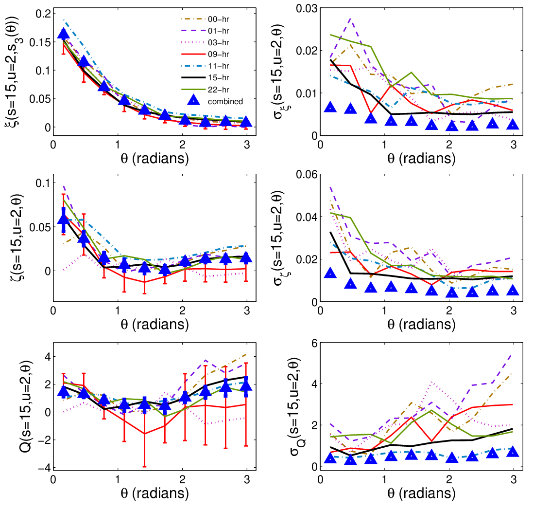
In Figure 6 we show measurements of the correlation functions in the sample for each WiggleZ region. Measurements in different regions are consistent within the statistical errors from cosmic variance and shot noise. On these scales we notice how small differences in and translate to larger discrepancies in . The noisiest 3-point functions are obtained in the smallest regions (in terms of volume), in this case the regions overlapping with the RCS2 survey. We will build a ‘combined’ set of correlation functions calculated by optimally weighting individual contributions of the regions.

To measure the diagonal errors and covariance matrices, ideally we require a large number of mock galaxy catalogues whose correlation functions have similar amplitude and shape dependence to the one observed in our data. However, this is not currently tractable for WiggleZ galaxies due to their low bias, which would necessitate many high-resolution simulations in a cosmological volume. In past studies we have used lognormal realisations (Blake et al., 2010) to generate a large number of mocks suited to match the WiggleZ 2-point amplitudes. Unfortunately, by their construction (from generating points with a particular 2-point distribution), these are not capable of reproducing the higher-order clustering of galaxies.
In this work, error measurements in each region are calculated from jack-knife resampling (Zehavi et al., 2005; McBride et al., 2011; Norberg et al., 2011). In this method we divide the whole volume of the sample in identical subsamples , and we then measure correlation functions for the whole volume minus the -th subsample times to get a set of correlated measurements. In our case, in all WiggleZ regions we take subregions of equal area (weighted by sky completeness), with an equivalent physical size of approx. (Mpc)3 at . The angular cut has the same area independent of region, as can be seen in Figure 1, thus some WiggleZ regions have more JK subregions than others, depending on their total area coverage.
In order to obtain the JK variance in each region, we measure each statistic (where can be the 2PCF or the 3PCF), subtracting one of the JK subregions in turn. Then we calculate the variance of the individual WiggleZ region as
| (10) |
where is the number of jack-knife subsamples, in region (see Table 1). Then, we calculate the correlations in the overall survey using inverse-variance weighting. For the statistic , this is calculated as
| (11) |
where is the variance of the statistic in the WiggleZ subregion (calculated in equation 10), taken from the jack-knife resampling method. is the number of WiggleZ regions we use for the calculation of the combined correlations. We do this for , and . In principle there should be no difference between calculating correlations using this method and measuring triplet counts across the whole survey; in practice our method is more computationally efficient and gives us extra systematics tests by allowing us to compare results region by region.
Overall diagonal errors and covariance matrices are calculated by jack-knife resampling the whole set of survey regions (see Figure 1). This way, we produce a catalogue of measurements. The variance of the correlations is calculated as
| (12) |
We also use this method to calculate the covariance matrix, which is used in the Maximum Likelihood approach to measure the galaxy bias and cosmological parameters.
4.2 The Combined WiggleZ 3PCF
Figure 7 shows the measurements of the redshift-space 2PCF , connected 3PCF and reduced 3PCF, , of WiggleZ galaxies (from optimally combining the seven independent regions) in all redshift slices for a range of scales , 15, 20 and 30 Mpc and shape as a function of . We have additionally measured the correlations using and , for a total of 120 configurations, which are shown in Appendix A.
We note qualitatively that we recover the same shape dependence of the galaxy 3PCF (mostly noticeable when looking at ) which has been observed for galaxies at low redshift (McBride et al., 2011; Marín, 2011), namely a bigger 3PCF amplitude at small and large , i.e the collapsed and elongated configurations. This ‘V-shape’ is more prominent for large scales and elongated shapes; it is a consequence of the morphology of galaxy structures varying from spherically-shaped clusters and groups on small 1 Mpc scales to filaments on the largest scales. This shape dependence of the 3PCF depends on the galaxy type under investigation. It has been observed in SDSS (Kayo et al., 2004; McBride et al., 2011) and 2dFGRS (Gaztañaga et al., 2005) that blue galaxies tend to have small 3PCF amplitudes on small scales and very pronounced V-shapes on large scales, compared to red galaxies and to galaxies, such as LRGs (Marín, 2011). Although at a different redshift, we find that the shape dependence of the WiggleZ 3PCF agrees with these lower redshift measurements.
We also note that on larger scales the behaviour of the reduced 3PCF for the most elongated shapes is more erratic, specially for the and redshift slices. This is due to the fact that as on large scales, the measurements of are less robust and its errors become non-Gaussian. But if we turn to analyze instead, we can see that it is adequately measured up to the largest scales shown here, Mpc.
Comparing the clustering signal in different redshift slices, we can see that in general the differences in the 3PCF are small and the signal is weaker than in the case of the central slice. This does not necessarily indicate that there is no evolution of the clustering of WiggleZ galaxies with redshift; the underlying dark matter clustering changes with redshift, and consequently the linear and non-linear bias factors evolve. From the 2PCF measurements we can estimate the evolution of the linear bias, and using the 3PCF we can also test if there is evolution in the non-linear bias parameter.
In Figure 8 we illustrate how the errors in our measurements vary with redshift by showing the 1- diagonal errors (from jack-knife resampling) of the 2PCF and 3PCF measurements for a selection of configurations ( Mpc and ) of our (combined) redshift samples. It can be clearly seen that measurements are more accurate in the central redshift slice () than in the outer ones. In these configurations, the relative error in the 2PCF is around , for the connected 3PCF the relative errors reach in the central redshift slice.

4.3 Covariance estimation

We estimate the correlations between measurements of the 2PCF and 3PCF by empirically calculating the covariance matrix. Using the jack-knife method, given a number of measurements in number of bins , a fractional error of a quantity for the sample can be written as
| (13) |
where in our case, if then and otherwise , and is the standard error on calculated using the jack-knife method. Then we calculate the correlation matrix (covariance matrix normalized by diagonal errors) as
| (14) |
As an example that shows the observed behaviour of all configurations at different redshift samples, we show in Figure 9 the correlation matrix of both and for the configurations with Mpc, and , 2 and 3. In this case the number of bins , making a matrix. We divide this matrix into four regions depicting the auto- and cross- correlations. In the case of the covariance we notice that although it is dominated by diagonal terms, the off-diagonal terms are important too; the white stripes (signaling high covariance) in the off-diagonal matrices ( where ) are triangles that share a similar . The -correlation matrix also shows important non-diagonal elements that are more correlated for the elongated shapes (a combination of true covariance and binning). The cross-covariance is small but needs to be considered in the analysis.
5 Constraints on Galaxy bias and
We compare the dark matter correlations measured in the GiggleZ simulations to the WiggleZ 2PCF and 3PCF in order to constrain the linear and non-linear bias parameters using the local bias model described in 3.3. In this analysis we assume all cosmological parameters are fixed, and fit for by scaling the amplitude of the dark matter correlations in the manner of equations (7) and (8), with all quantities measured in redshift space. We want to emphasize that since we are using N-body simulation measurements to compare to our galaxy correlations, and not an analytical model, the only cosmological parameter we can modify is through the ratio , where the fiducial value corresponds to the one used in the GiggleZ simulation .
5.1 Methods
We carry out a Maximum Likelihood parameter estimation test, where we look to minimize the quantity
| (15) |
where is the number of triangular configurations used; we have distances where we measure the 2PCF of , and triangles where we measure the 3PCF, therefore we have elements in our covariance matrix. The value of is the difference between the correlation measured and the biased DM correlation:
| (16) | |||||
| (17) |
where and are given by eqs. (7,8).
In order to invert the covariance matrix we use the approach of Gaztañaga & Scoccimarro (2005) and repeated in several 3PCF works (Gaztañaga et al., 2005; McBride et al., 2011; Marín, 2011), of employing only the highest eigenmodes of the covariance matrix to minimize effects of numerical noise. We employ the Singular Value Decomposition method, where our normalized covariance matrix can be decomposed (and where for a symmetric matrix), where the diagonal matrix stores the eigenvalues in decreasing order, and the columns of the matrix stores the eigenmodes of . When inverting the matrix , (where ) we need to discard some of these eigenmodes, meaning set some . Firstly, we use a finite number of jack-knife samples to estimate our covariance. Since using jack-knife samples assumes the statistical independence of the subsamples, the jack-knife regions should have a larger spatial extent than the largest scales studied. In our case we use JK regions because our largest scales are of the order Mpc. However, we are using a large number of 2PCF and 3PCF measurements, and generally , which will make our matrix singular for modes (see Press et al. 1992 for instance). Therefore, all those eigenmodes have to be discarded. A second cut comes from the fact that even though the covariance matrix is not singular when the first cut is applied, there are still eigenvalues with very low numerical value, which will make unstable the inversion of with (Gaztañaga & Scoccimarro, 2005). Adding these unstable modes, as explained by these authors and later in section 5.2, is equivalent to introducing artificial ‘signal’ to our measurements that will bias our fits.


We also have to set the minimum and maximum scale of the model fit. In our analysis this means that we chose configurations with the third size in a range . The minimum scale is given by the range of validity of the local bias model. The maximum scale could be set by systematics in the selection function or when the correlation signal is weak. In Figures 10, 11 and 12 we show how our choices of the number of eigenvalues used, the values of and respectively affect our constraints for our sample.
We wish to make a sensible default choice for these options and establish that our essential conclusions are not very sensitive to this choice. Figure 10 investigates the dependence of our results on the number of eigenmodes included, fixing Mpc and Mpc. We observe that if we use a small number of eigenvalues we have large variations in the best fit values and poor constraints, especially in ; then there is a range when the number of eigenvalues used is where our results are insensitive, and when we include modes with we again have unstable behaviour. In this figure we also consider the dependence of the minimum per degree of freedom on the number of eigenmodes employed, where the degrees of freedom are equal to the eigenmodes used minus the number of parameters we seek to constrain. We note that good fits are produced for a wide range of choices. We can also estimate the total signal-to-noise () ratio of the modes used as (Gaztañaga & Scoccimarro, 2005):
| (18) |
where when , and when .
Our conclusion from this analysis is that any systematic fluctuations in our parameter measurements do not dominate the statistical errors for a wide range of choices. Our default fits are performed for an eigenmode cut and a fitting range Mpc and Mpc for the and 0.68 slices, and Mpc for the sample.
Another aspect to consider in our analysis is that the measured redshifts in our survey contain a small fraction of ‘redshift blunders’ (Blake et al., 2010), failures that tend to wash out the clustering we measure in our galaxy field. This redshift blunder fraction is for the and 0.55 redshift slices, and for the outer slice; the correction to the 2PCF (since ) is to multiply the data and errors by , meaning that the clustering amplitude increases; and the correction to the 3-pt function (where ) is .
5.2 Constraints at
 |
 |
In Figure 13 we show the measurements of , and in the redshift slice. The measured linear bias, , agrees with values obtained for WiggleZ galaxies using other methods (Blake et al., 2011b; Contreras et al., 2012), using 2-point statistics, where in our study we additionally marginalise over all values of . We detect a significantly non-zero value for the non-linear bias .
We measure the amplitude of fluctuations with 10% accuracy and find that our results agree with independent predictions, based on cosmological parameter measurements from the CMB in a CDM model. It is important to note that these estimates are independent of any other observable than the galaxy clustering itself. Extrapolated to , our measurements of from WiggleZ galaxies are consistent with conclusions from 3PCF measurements of other tracers such as the LRGs (Marín, 2011), which provides evidence that this method is robust against the type of galaxy used.
As is shown in Table 2, the empirical bias model is an adequate fit to the data, and that can be graphically seen in the right-hand plots of Figure 13, where we show the biased dark matter , which in our model depends on the bias parameters but not on :
| (19) |
We can see that our galaxy bias model is adequate on all scales, but our fits are mainly driven by the and 15 Mpc configurations, which have the highest signal-to-noise ratio.
| dof | |||||
|---|---|---|---|---|---|
| 0.35 | 1.10 | 3.25 | |||
| 0.55 | 0.96 | 4.99 | |||
| 0.68 | 0.82 | 4.62 |
5.3 Constraints at different redshifts
We repeated the analysis of the correlation functions for the other two redshift slices in order to get constraints on the bias parameters and as a function of redshift. In Table 2 we show our results. In general we can see that there is clear trend in all the parameters with redshift, and that from the values of dof, our model of the bias provides a good fit. We also estimated the covariance between the best-fit parameters in different redshift slices, expected due to the overlap between redshift samples. In order to make this measurement we fitted the bias parameters and to each delete-1 jack-knife sample, obtaining sets of best fit parameters which we used to construct a covariance matrix. We show the correlation matrix of these parameters in Figure 14. We observe that in any individual redshift slice there is a positive correlation between and and a negative correlation between these parameters and . Although there is overlap in the redshifts of the samples studied, the correlation coefficients between best-fit parameters in separate redshift slices are small.

In the following we study the change of the bias parameters and with redshift in more detail.
 |
 |
5.3.1 Constraints of WiggleZ bias
Figure 15 displays the change of the galaxy bias with redshift. Due to our selection criteria, we are not necessarily selecting the same population of galaxies at different redshifts (Li et al., 2012), specially at redshifts . Therefore we only can make general statements about evolution of the bias of WiggleZ galaxies. For the linear bias it can be seen that there is an upward trend of bias with redshift, consistent with what is expected for the evolution of halos of a given mass: massive objects are less common in older times, and therefore more biased.
In order to compare our measured bias evolution to the expectation of simple models, we also plot the evolution of the bias of dark matter halos of fixed mass with redshift in the halo model. These are given by the analytical expectation using Sheth-Tormen mass functions (Sheth et al., 2001) for the dark matter halos, and the linear and non-linear bias from the work of Scoccimarro et al. (2001). Since our galaxies are a subsample of the total population, with a particular colour and luminosity selection, we do not expect that they should follow exactly one track of evolution, but in any case, our measured bias evolution seems to agree with those galaxies living in halos with masses .
In our measurements and in the halo model, it is expected that when a galaxy tracer has a linear bias , it should have a small but significantly negative non-linear bias . In the right panel of Figure 15 we show the evolution of the WiggleZ galaxies’ non-linear bias. These have negative values, and their trend agrees with what is expected of halos. A more detailed analysis using Halo Occupation Distribution models is needed to have a complete picture of how WiggleZ galaxies populate dark matter halos; this is beyond the scope of this paper.
5.3.2 Evolution of cosmic growth
In Figure 16 we plot our measurements of as a function of redshift from the WiggleZ survey data. In linear theory, the value of is calculated as
| (20) |
where is the Fourier transform of a tophat window of radius Mpc. The linear power spectrum evolves as , where is a reference redshift (e.g., the redshift of recombination) and is the linear growth factor, obtained from the solution to the linearized equations of motion of primordial overdensities (Peebles, 1980; Bernardeau et al., 2002). The evolution of the linear growth factor depends on the parameters of the cosmological model (Lahav & Suto, 2004). Thus, we obtain
| (21) |
Therefore, measurements from the 2PCF and 3PCF can be used to study the evolution of the linear growth factor.
As predicted by the standard cosmological model, the value of we measure decreases at earlier times, in agreement with the WMAP5 cosmological parameters. Assuming a flat CDM model with we find that when extrapolated to the present epoch, . Our results also agree with the latest estimation of using BOSS/SDSS-LRGs passive galaxies from Tojeiro et al. (2012); modelling the evolution of the linear bias for their particular population they find similar values to ours. However, in our work we need to make no assumptions about the evolution of the bias, just in the validity (range of scales) of the empirical bias model we adopt. We also find agreement with other measurements of from the 3PCF of the SDSS LRG sample (Marín, 2011); they find , consistent with our measurements at the same effective redshift.

We also plot in Figure 16 the evolution of in two different models of flat universes, an Einstein-de Sitter model (flat =1) and another one with no matter content, just cosmological constant. As WMAP5 (Komatsu et al., 2009) measured the amplitude of CMB perturbations at the epoch of recombination , we normalize at that redshift for the three cosmologies shown here. We find that an Einstein-de Sitter universe is disfavoured ( for one parameter fit) when combining measurements of the three WiggleZ redshift samples, as well as spacially flat models with low matter content ( for ).
6 Summary and Conclusions
We have measured the redshift space two- and three- point clustering statistics for the WiggleZ galaxies and obtained constraints on the linear and non-linear galaxy bias and the cosmological parameter at three different epochs. Our results can be summarized as follows:
- •
We obtain significant measurements of the WiggleZ 3PCF, recovering its shape dependence on large scales, spanning a wide redshift range for all regions and subregions (in angle and redshift) of the galaxy sample.
- •
These measurements are in agreement with standard models for the growth of structure driven by gravitational clustering, reflecting the morphology of the clustering large-scale structures, i.e. the ‘cosmic web’.
- •
Using a simple local bias parameterization along with an empirical treatment of redshift-space distortions of the correlation functions, we get constraints on the bias parameters as a function of redshift. Our estimation of the linear bias agrees with evolution of dark matter halos .
- •
For all our redshift samples, we detect a significant non-zero (negative) non-linear bias, also consistent with the models for the non-linear bias evolution of halos of masses .
- •
We also constrain the evolution of with redshift, and by extension, the evolution of the linear growth factor. We find that our measurements are consistent with the predictions of a WMAP5 CDM concordance cosmology and with measurements from other methods and observables.
The improvement in the measurements of the higher-order correlations in the last ten years has been dramatic, and it is remarkable that we can now measure the 3PCF using galaxies up to redshift . Although the signal-to-noise ratio of the WiggleZ 3PCF is weaker than lower-redshift measurements from the SDSS Main Sample (McBride et al. 2011; McBride et al. 2011 ) and SDSS LRG sample (Kulkarni et al., 2007; Marín, 2011), we nonetheless have extended the utility of higher-order correlations functions to , using the WiggleZ survey data. We note that using jack-knife resampling for error estimation probably overestimates the variance on large scales (Marín, 2011); our measurements would be improved by the availability of mock galaxy catalogues. At the same time, with improved statistics we need to improve our modelling of redshift space distortions and small-scale effects in order to extract as much information as possible from the higher-order correlations.
Also, improved modelling would help to combine 3PCF measurements with other observables such as clustering and lensing (Mandelbaum et al., 2012, see), 2-dimensional RSD 2-point statistics, or the passive galaxies method (Tojeiro et al., 2012).
In the near future, with improved measurement techniques and with bigger surveys, we will be able to use these techniques to measure the growth factor accurately and discriminate between CDM model and modified gravity models (Linder & Cahn, 2007).
Acknowledgements
We thank Eyal Kazin for fruitful discussions and suggestions, and to the anonymous referee and for valuable comments and suggestions. We acknowledge financial support from the Australian Research Council through Discovery Project grants which have funded the positions of MP, GP, TD and FM. SMC acknowledges the support of the Australian Research Council through a QEII Fellowship. CB acknowledges the financial support of the ARC through a Future Fellowship award. We are also grateful for support from the Centre for All-sky Astrophysics, an Australian Research Council Centre of Excellence funded by grant CE11000102.
GALEX (the Galaxy Evolution Explorer) is a NASA Small Explorer, launched in April 2003. We gratefully acknowledge NASA’s support for construction, operation and science analysis for the GALEX mission, developed in co-operation with the Centre National d’Etudes Spatiales of France and the Korean Ministry of Science and Technology.
Finally, the WiggleZ survey would not be possible without the dedicated work of the staff of the Australian Astronomical Observatory in the development and support of the AAOmega spectrograph, and the running of the AAT.
References
- Adelman-McCarthy et al. (2006) Adelman-McCarthy J. K., et al., 2006, ApJS, 162, 38
- Bardeen et al. (1986) Bardeen J. M., Bond J. R., Kaiser N., Szalay A. S., 1986, ApJ, 304, 15
- Barriga & Gaztañaga (2002) Barriga J., Gaztañaga E., 2002, MNRAS, 333, 443
- Berlind & Weinberg (2002) Berlind A. A., Weinberg D. H., 2002, ApJ, 575, 587
- Bernardeau et al. (2002) Bernardeau F., Colombi S., Gaztañaga E., Scoccimarro R., 2002, PhysRep., 367, 1
- Beutler et al. (2011) Beutler F. et al., 2011, MNRAS, 416, 3017
- Blake et al. (2010) Blake C., et al., 2010, MNRAS, 406, 803
- Blake et al. (2011a) Blake C., et al., 2011a, MNRAS, 415, 2892
- Blake et al. (2011b) Blake C., et al., 2011b, MNRAS, 415, 2876
- Cole et al. (2005) Cole S. et al., 2005, MNRAS, 362, 505
- Contreras et al. (2012) Contreras C., et al., 2012, MNRAS submitted
- Cooray & Sheth (2002) Cooray A., Sheth R., 2002, PhysRep., 372, 1
- Drinkwater et al. (2010) Drinkwater M. J., et al., 2010, MNRAS, 401, 1429
- Eisenstein et al. (2005) Eisenstein D. J., et al., 2005, ApJ, 633, 560
- Eke et al. (1996) Eke V. R., Cole S., Frenk C. S., 1996, MNRAS, 282, 263
- Feldman et al. (1994) Feldman H. A., Kaiser N., Peacock J. A., 1994, ApJ, 426, 23
- Fosalba et al. (2005) Fosalba P., Pan J., Szapudi I., 2005, ApJ, 632, 29
- Frieman & Gaztanaga (1994) Frieman J. A., Gaztanaga E., 1994, ApJ, 425, 392
- Fry & Gaztanaga (1993) Fry J. N., Gaztanaga E., 1993, ApJ, 413, 447
- Fu et al. (2008) Fu L. et al., 2008, A&A, 479, 9
- Gardner et al. (2007) Gardner J. P., Connolly A., McBride C., 2007, in R. A. Shaw, F. Hill, & D. J. Bell ed., Astronomical Society of the Pacific Conference Series Vol. 376, Astronomical Data Analysis Software and Systems XVI. p. 69
- Gaztañaga et al. (2005) Gaztañaga E., Norberg P., Baugh C. M., Croton D. J., 2005, MNRAS, 364, 620
- Gaztañaga & Scoccimarro (2005) Gaztañaga E., Scoccimarro R., 2005, MNRAS, 361, 824
- Gaztanaga et al. (2008) Gaztanaga E., Cabre A., Castander F., Crocce M., Fosalba P., 2008, ArXiv e-prints, 807
- Gilbank et al. (2011) Gilbank D. G., Gladders M. D., Yee H. K. C., Hsieh B. C., 2011, AJ, 141, 94
- Guo et al. (2013) Guo H., Li C., Jing Y. P., Boerner G., 2013, ArXiv e-prints
- Jing & Borner (1997) Jing Y. P., Borner G., 1997, A&A, 318, 667
- Jing & Börner (2004) Jing Y. P., Börner G., 2004, ApJ, 607, 140
- Kaiser (1987) Kaiser N., 1987, MNRAS, 227, 1
- Kayo et al. (2004) Kayo I. et al., 2004, PASJ, 56, 415
- Kazin et al. (2010) Kazin E. A. et al., 2010, The Astrophysical Journal, 710, 1444
- Kilbinger et al. (2012) Kilbinger M. et al., 2012, ArXiv e-prints
- Komatsu et al. (2009) Komatsu E., et al., 2009, ApJs, 180, 330
- Kulkarni et al. (2007) Kulkarni G. V., Nichol R. C., Sheth R. K., Seo H.-J., Eisenstein D. J., Gray A., 2007, MNRAS, 378, 1196
- Lahav & Suto (2004) Lahav O., Suto Y., 2004, Living Reviews in Relativity, 7, 8
- Landy & Szalay (1993) Landy S. D., Szalay A. S., 1993, ApJ, 412, 64
- Li et al. (2012) Li I. H. et al., 2012, ApJ, 747, 91
- Lin et al. (2011) Lin H. et al., 2011, ArXiv e-prints
- Linder & Cahn (2007) Linder E. V., Cahn R. N., 2007, Astroparticle Physics, 28, 481
- Mandelbaum et al. (2012) Mandelbaum R., Slosar A., Baldauf T., Seljak U., Hirata C. M., Nakajima R., Reyes R., Smith R. E., 2012, ArXiv e-prints
- Marín (2011) Marín F., 2011, ApJ, 737, 97
- Marín et al. (2008) Marín F. A., Wechsler R. H., Frieman J. A., Nichol R. C., 2008, ApJ, 672, 849
- Martin et al. (2005) Martin D. C., et al., 2005, ApJl, 619, L1
- McBride et al. (2011) McBride C. K., Connolly A. J., Gardner J. P., Scranton R., Newman J. A., Scoccimarro R., Zehavi I., Schneider D. P., 2011, ApJ, 726, 13
- McBride et al. (2011) McBride C. K., Connolly A. J., Gardner J. P., Scranton R., Scoccimarro R., Berlind A. A., Marín F., Schneider D. P., 2011, ApJ, 739, 85
- Nichol et al. (2006) Nichol R. C., et al., 2006, MNRAS, 368, 1507
- Norberg et al. (2001) Norberg P., et al., 2001, MNRAS, 328, 64
- Norberg et al. (2011) Norberg P., Gaztañaga E., Baugh C. M., Croton D. J., 2011, MNRAS, 418, 2435
- Pan & Szapudi (2005) Pan J., Szapudi I., 2005, MNRAS, 362, 1363
- Peacock et al. (2001) Peacock J. A., et al., 2001, Nature, 410, 169
- Peebles (1980) Peebles P. J. E., 1980, The Large-Scale Structure of the Universe. Princeton University Press
- Peebles & Groth (1975) Peebles P. J. E., Groth E. J., 1975, ApJ, 196, 1
- Percival et al. (2007) Percival W. J. et al., 2007, ApJ, 657, 645
- Poole et al. (2012) Poole G., et al., 2012, in preparation
- Press & Schechter (1974) Press W. H., Schechter P., 1974, ApJ, 187, 425
- Press et al. (1992) Press W. H., Teukolsky S. A., Vetterling W. T., Flannery B. P., 1992, Numerical Recipes in C. Cambridge University Press
- Ross et al. (2006) Ross A. J., Brunner R. J., Myers A. D., 2006, ApJ, 649, 48
- Rozo et al. (2010) Rozo E. et al., 2010, ApJ, 708, 645
- Sánchez et al. (2012) Sánchez A. G., et al., 2012, MNRAS, 425, 415
- Scoccimarro et al. (1999) Scoccimarro R., Couchman H. M. P., Frieman J. A., 1999, ApJ, 517, 531
- Scoccimarro et al. (2001) Scoccimarro R., Sheth R. K., Hui L., Jain B., 2001, ApJ, 546, 20
- Sefusatti & Scoccimarro (2005) Sefusatti E., Scoccimarro R., 2005, Phys. Rev. D, 71, 063001
- Sharp et al. (2006) Sharp R., et al., 2006, in Society of Photo-Optical Instrumentation Engineers (SPIE) Conference Series.
- Sheth et al. (2001) Sheth R. K., Mo H. J., Tormen G., 2001, MNRAS, 323, 1
- Smith et al. (2003) Smith R. E. et al., 2003, MNRAS, 341, 1311
- Smith et al. (2008) Smith R. E., Sheth R. K., Scoccimarro R., 2008, Phys. Rev. D, 78, 023523
- Springel et al. (2001) Springel V., White S. D. M., Tormen G., Kauffmann G., 2001, MNRAS, 328, 726
- Szapudi & Szalay (1998) Szapudi S., Szalay A. S., 1998, ApJl, 494, L41
- Tojeiro et al. (2012) Tojeiro R., et al., 2012, MNRAS, 424, 2339
- Verde et al. (2002) Verde L. et al., 2002, MNRAS, 335, 432
- White & Frenk (1991) White S. D. M., Frenk C. S., 1991, ApJ, 379, 52
- White & Rees (1978) White S. D. M., Rees M. J., 1978, MNRAS, 183, 341
- Yang et al. (2002) Yang X., Mo H. J., van den Bosch F. C., 2002, preprint, astro-ph/0207019
- Zehavi et al. (2005) Zehavi I., et al., 2005, ApJ, 630, 1
- Zehavi et al. (2011) Zehavi I. et al., 2011, ApJ, 736, 59
Appendix A WiggleZ 3PCF measurements of isosceles and very elongated triangles

In Figure 17 we plot results of the WiggleZ correlation functions measured for isosceles configurations, where , for the three redshift slices we studied. In these configurations, the third side length runs from on very small angles , where the bias model we use is no longer valid due to high nonlinearities. Since the third triangle side covers a large range of scales, for purposes of plotting we show the absolute values of the 2PCF and connected 3PCF on a logarithmic scale, while is shown on a linear scale (which can take positive or negative values). We can observe first that in general the errors in these measurements are smaller compared with the ones we showed in Figure 5 for the configurations. As in the configurations, there is no significant evolution in the amplitude of the correlation values. The 3PCF of equilateral triangles (, ) is small and even negative, as expected when galaxies cluster in filamentary structures on the largest scales.

In Figure 18 we plot results of the WiggleZ correlation functions measured on very elongated configurations, where , for the three redshift slices we studied. For these configurations the signal-to-noise ratio is much smaller than in other configurations, specially on large . For the redshift slice (green dashed line), and are poorly measured on the largest scales, justifying our decision to use a maximum separation smaller than that adopted for the other two redshift slices. Notice that we reach scales where the BAO features could in principle be observed Mpc, but the WiggleZ low galaxy bias makes it difficult to achieve a significant detection that could be used to constrain cosmological parameters (as claimed by Gaztanaga et al., 2008, for SDSS LRGs).