An asymptotic parallel-in-time method for highly oscillatory PDEs

We present a new algorithm to integrate nonlinear PDEs that exhibit scale separation in time. We focus on time scale separation of a highly oscillatory nature, where standard (explicit or implicit) time-stepping methods often require time steps that are on the order of the fastest oscillation to achieve accuracy. This type of equation arises in numerous scientific applications, including the large-scale simulations of the ocean and atmosphere that serve as the primary motivation of this paper [7, 8].

In particular, we consider computing solutions to equations of the form

where the linear operator $\mathcal{L}$ has pure imaginary eigenvalues, the nonlinear term $\mathcal{N}\left(\mathbf{u}\right)$ is of polynomial type, the operator $\mathcal{D}$ encodes some form of dissipation, and $\epsilon$ is a small non-dimensional parameter. For notational simplicity, we let $\mathbf{u}\left(t\right)$ denote the spatial (vector-valued) function $\mathbf{u}\left(t,\cdot\right)=\left(u_{1}\left(t,\cdot\right),u_{2}\left(t,\cdot\right),\ldots\right)$. The operator $\epsilon^{-1}\mathcal{L}$ results in temporal oscillations on an order $\mathcal{O}\left(\epsilon\right)$ time scale, and generally necessitates small time steps if standard numerical integrators are used.

Our approach for integrating (1.1) uses a variant of the parareal algorithm [26], which is a parallel-in-time method that relies on a cheap coarse solver for computing in serial a solution with low accuracy, and a more expensive fine solver for iteratively refining the solutions in parallel. The key novelty in this paper is to replace the numerical coarse solution of the full equations (1.1) with a locally asymptotic approximation of (1.1). This enables us to effectively bypass the Nyquist constraint imposed by the fastest oscillations, and acheive much greater parallel speedup. Examples on the rotating shallow water equations—a standard benchmark against which to test new algorithms in geophysical fluid applications—demonstrate that this approach holds promise for increasing the accuracy and speed of geophysical fluid simulations. In fact, we find (see Section 6.2) that this approach allows us to take step sizes $\Delta T\gg\epsilon$ that are significantly larger than if alternative schemes are used for the coarse solver, including exponential integrators and split-step methods (which solve the stiff linear terms exactly). In the context of large-scale simulations of the ocean and atmosphere, the gains achieved from spatial parallelization alone are beginning to saturate, and the results in this paper are a preliminary effort toward achieving greater efficiency.

We first describe the standard parareal method in more detail, and some of the challenges for acheiving high parallel speedup for problems of the form (1.1). The basic approach of the parareal method is to take large time steps $\Delta T$ in serial using a coarse integrator of (1.1), and to iteratively refine the solutions in parallel using small time steps $\Delta t$ and a more accurate integrator. This can result in significant speedup in real (wall-clock) time if the parareal iterations converge rapidly, and either the ratio $\Delta T/\Delta t$ of coarse and fine step sizes is large, or the cost of the coarse solver is much cheaper than that of the fine solver (see Section 5 for more details). Early applications of the parareal method include simulations of molecular dynamics [4], the Navier Stokes equation [17], and quantum control problems [28]; additional references can be found in [37]. Although the parareal method has been most widely used for parabolic-type PDEs, it has also been analyzed and used for accurate simulation of first and and second order hyperbolic systems (cf. [16], [18], and [10]). A recent variant of the parareal method also allows for the accurate long-time evolution of Hamiltonian systems [25]. Finally, general convergence results for the parareal algorithm can be found in [19, 5] ([19] also numerically demonstrates convergence on the Lorenz equations, which is of particular relevance to geophysical fluid problems).

Despite the many successes of the parareal method, a basic obstacle remains for equations of the form (1.1): namely, the step size $\Delta T$ for a coarse integrator that is based on a standard method generally must satisfy $\Delta T=\mathcal{O}\left(\epsilon\right)$ in order to achieve any accuracy at all (which is a prerequisite for convergence of the parareal method). In practice, this can mean that the coarse integrator in the parareal method must use very small time steps for solving (1.1), and the parallel speedup can be minimal. There are, however, some types of highly oscillatory PDEs where numerical integrators have been developed that can take much larger time steps $\Delta T\gg\epsilon$ (cf. [20]).

In this paper, we use a numerically computed ’locally slow’ solution that is based on the underlying asymptotic structure of (1.1), and which can allow step sizes $\Delta T\gg\epsilon$ significantly larger than the Nyquist constraint imposed by the $\mathcal{O}\left(\epsilon\right)$ temporal oscillations (and thus a potentially significant parallel speedup). A basic observation behind efficiently constructing a slow solution is that the solution $\mathbf{u}\left(t\right)$ to (1.1) has the asymptotic approximation $\mathbf{u}\left(t\right)=\exp\left(-t/\epsilon\mathcal{L}\right)\overline{\mathbf{u}}\left(t\right)+\mathcal{O}\left(\epsilon\right)$ (cf. [29], [30], [38]), where the slowly varying function $\overline{\mathbf{u}}\left(t\right)$ satisfies a reduced equation of the form

Here the nonlinear term $\overline{N}\left(\overline{\mathbf{u}}\right)$ is given by the time average

We emphasize that the above time averaging is performed with $\overline{\mathbf{u}}\left(t\right)$ held fixed. Similarly,

Note that $\overline{\mathbf{u}}\left(t\right)$, and its time derivatives, are formally bounded independently of $\epsilon$, and thus significantly larger time steps $\Delta T\gg\epsilon$ can be taken to evolve (1.2). Section 4 also discusses how a numerical integrator based on a finite version of the time averages (1.3) and (1.4) can be interpreted as a smoothed type of integrating factor method, and allows accuracy even when there is no scale sepatation in time (i.e. $\epsilon=\mathcal{O}\left(1\right)$); this is useful when the scale separation is localized in space, and where it is desirable to have a time step that is constrained only by the slow dynamics.

Despite the many successes of the above averaging procedure in elucidating important qualitative features (see e.g. [30] and [38] for geophysical fluid dynamics applications), in practice this approach may not be accurate enough for moderately small values of $\epsilon$ (e.g. $\epsilon=10^{-2}$ is typical in geophysical fluid applications), where the implicit constant hidden in the $\mathcal{O}\left(\epsilon\right)$ notation can be significant [36]. Since the parameter $\epsilon$ is typically fixed in idealized applications, the resulting asymptotic approximation cannot be refined without some additional approach. Another limitation is that the asymptotic approximation (1.2) is generally only valid on an $\mathcal{O}\left(1\right)$ time interval, and this situation is usually not improved by adding more terms in the asymptotic expansion. For many applications, it is therefore necessary to refine this approach in order to approximate (1.1) with a given target accuracy and on longer time intervals.

Our approach for computing the asymptotic approximation (1.2)—for the purpose of constructing a slow solution—is based on evaluating the time averages $\overline{\mathcal{N}}\left(\overline{\mathbf{u}}\left(t\right)\right)$ and $\overline{\mathcal{D}}\overline{\mathbf{u}}\left(t\right)$ numerically; this approach has also been used in [6] to solve Hamiltonian systems more efficiently (see also [31] and [21] for related approaches in geophysical simulations). More generally, our numerical scheme for (1.2) is an instance of the Heterogeneous Multiscale Method (HMM) (cf. [12, 15, 2, 1] for selective applications to highly oscillatory problems), which is a very general framework for efficiently computing approximations to problems that exhibit multiple spatial or temporal scales; a review of HMM can be found in [13]. The basic idea is that, by integrating in time against a carefully chosen smooth kernel, the time average can be performed over a window of length $T_{0}=T_{0}\left(\epsilon\right)\ll 1/\epsilon$; therefore, the overall cost of evolving (1.2) is asymptotically smaller than the cost of computing (1.1) directly, and can lead to arbitrarily large efficiency gains. In problems arising in geophysical fluid applications, the value $\epsilon$ may only be moderately small (e.g. $\epsilon\approx 10^{-2}$), and in such cases numerically computing the average (1.3) can be as costly as explicitly integrating the full equation (1.1). However, the numerical average can itself be performed in an embarassingly parallel manner (see Section 2), and thus is not expected to impact the overall (wall-clock) speed of the algorithm. Finally, we remark that for solutions that develop sharp gradients, it may be necessary to use the modified version of the parareal method explored in [10]. However, this is beyond the scope of this paper.

The idea of using a coarse solution based on a modified equation is not new, and the possibility has been mentioned early on in the parareal literature (cf. [37]). In [27] and [14], multi-scale versions of the parareal method are developed for, respectively, deterministic and stochastic chemical kinetic simulations; in [14], the coarse solver is based on a deterministic (macroscopic) approximation. A recent paper [24] applies a version of the parareal method to systems of ODEs that exhibit fast and slow components. The multi-scale coarse solver in [24] uses a projection onto the slow, low-dimensional manifold, and examples are provided for singularly perturbed ODEs with dissipative-type scale separation. In contrast to [27], [14], and [24] , here we investigate this procedure for a model nonlinear PDE whose scale separation is of a highly oscillatory nature, and where methods that work well for stiff dissipative problems (e.g. implicit or exponential integrators) generally fail to impart significant speedup. Moreover, the asymptotic approximation (1.2) to (1.1) cannot be computed explicitly in most cases, and this necessitates using additional techniques. The locally asymptotic solver developed here works even when there is no scale separation, which is an important feature when the time scale separation is a function of space and time (as occurs in some geophysical fluid applications); in this case, the time step in the coarse, asymptotic solution is only constrained by the slow dynamics.

In Section 2, we present a version of the Heterogeneous Multiscale Method that is appropriate for efficiently computing the asymptotic approximation (1.2). We then present in Sections 3 a variant of the parareal method that is based on replacing the coarse solver with a locally asymptotic approximation. Section 4 shows that, by averaging over a scale on which the slow dynamics is occuring, this HMM-type coarse solution is able to achieve accuracy even when there is no scale separation. We provide complexity bounds for this algorithm, which demonstrate that the parallel speedup increases arbitrarily as $\epsilon$ decreases. We also present error bounds that are based on the analysis in [19] and [5], and that demonstrate convergence of the method under reasonable assumptions. Finally, Section 6.2 discusses some numerical experiments on the (one-dimensional) rotating shallow water equations, which serve as a standard first test for new numerical algorithms in geophysical applications. Our experiments show that, in contrast to standard versions of the parareal algorithm, the algorithm can converge to high accuracy in few iterations even when large time steps $\Delta T\gg\epsilon$ are taken for the coarse solution. In fact, compared to the exponential time differencing method (ETDRK4), the integrating factor method, and Strang splitting (cf. [9], [22], and [23])—all of which integrate the stiff linear term $\epsilon^{-1}\mathcal{L}$ exactly—our algorithm yields an estimated parallel speedup of $\approx 100$ for the physically realistic value of $\epsilon=10^{-2}$. We also show that, for $\epsilon=10^{-2}$, this parallel speedup is at least $10$ times greater than the speedup that can be achieved by using the standard parareal method with ETDRK4, OIFS, or Strang splitting as the coarse solver. Finally, we demonstrate that the asymptotic parareal method yields high accuracy even when $\epsilon=1$ (i.e. in the absense of scale separation), and with a parallel speedup that is comparable to using the standard parareal method with ETDRK4, OIFS, or Strang splitting as the coarse solver. Using a coarser spatial discretization in the asymptotic solver may also result in even greater efficiency gains.

We use the Heterogeneous Multiscale Method (HMM) to solve (1.2), which relies on computing the averages (1.3) and (1.4) numerically (see also [6]). The key idea is that, by averaging in time with respect to an appropriate smooth kernel and over a carefully selected window length $T_{0}=T_{0}\left(\epsilon\right)$, the cost is asymptotically smaller than $1/\epsilon$ (which is the cost of solving the full equation (1.1) on an $\mathcal{O}\left(1\right)$ time interval). Once such time averages can be computed, then large step sizes $\Delta T\gg\epsilon$, coupled with a standard numerical integrator, can be taken to evolve (1.2). For simplicity, we restrict our discussion to computing the time average (1.3) (in fact, for the equations we consider here, the operators $\mathcal{L}$ and $\mathcal{D}$ commute, and so the average $\overline{\mathcal{D}}$ in (1.4) satisfies $\overline{\mathcal{D}}=\mathcal{D}$).

The basic approach for computing the time average (1.3) involves the following approximations:

The smooth kernel $\rho\left(s\right)$, $0\leq s\leq 1$, is chosen so that the length $T_{0}=T_{0}\left(\epsilon\right)$ of the time window over which the averaging is done is as small as possible, and that the error introduced by using the trapezoidal rule is negligible (see e.g. [15] and [11] for an error analysis).

More formally, we define the finite time average

Then we need to choose the kernel $\rho\left(s\right)$ and the parameters $T_{0}=T_{0}\left(\epsilon\right)$ and $\overline{M}$ so that the truncation error,

and the discretization error,

are smaller than our desired approximation tolerance. This can be accomplished by requiring that the kernel $\rho\left(s\right)$ satisfies $\rho^{\left(m\right)}\left(0\right)=\rho^{\left(m\right)}\left(1\right)=0$, $m=0,1,\ldots$ It will also be convenient for comparison with Section 4 to change variables $s\rightarrow s/\epsilon$ in the integrand in (2.2) to obtain the equivalent form

To better understand the role of $\rho\left(s\right)$ and the parameters $T_{0}$ and $\overline{M}$, we informally analyze the above averaging procedure in more detail. First, since we are assuming that the nonlinear operator $\mathcal{N}$ in (1.3) is of polynomial type and $\mathcal{L}$ has pure imaginary eigenvalues, we can (in principle) expand $\overline{\mathbf{u}}\left(t\right)$ in terms of eigenfunctions of $\mathcal{L}$ and express the nonlinear term in the form

Here the pure imaginary numbers $i\lambda_{n}$ are linear combinations of the eigenvalues of $\mathcal{L}$, and the set $\lambda_{n}=0$ corresponds to resonant interactions (see Section 6.1 for a concrete example in the context of the rotating shallow water equations). In fact, using the definition of the averaging $\overline{\mathcal{N}}\left(\overline{\mathbf{u}}\left(t\right)\right)$ operator and the above decomposition, we see that

To compare this to the finite time average $\overline{\mathcal{N}}_{\rho,T_{0}}\left(\overline{\mathbf{u}}\left(t\right)\right)$, use (2.3) to express this as

Comparing $\overline{\mathcal{N}}_{\rho,T_{0}}\left(\overline{\mathbf{u}}\left(t\right)\right)$ and $\overline{\mathcal{N}}\left(\overline{\mathbf{u}}\left(t\right)\right)$, we therefore require that

In order to satisfy (2.4) with a time window length $T_{0}$ as small as possible, we choose a smooth kernel $\rho\left(s\right)$ that satisfies $\rho^{\left(m\right)}\left(0\right)=\rho^{\left(m\right)}\left(1\right)=0$. Repeated integration by parts shows that

In particular, the above calculation indicates that choosing a time window $T_{0}\left(\epsilon\right)=\epsilon^{-r}$, $0<r<1$, can formally yield an error

Moreover, repeated integration by parts, coupled with the Euler–Maclaurin formula, also shows that the error induced from the trapezoidal rule is similarly small,

One commonly used choice of kernel function is given by

where the constant $C$ is such so that $\left\|\rho\right\|_{1}=1$.

Notice that, compared to the asymptotic cost $\epsilon^{-1}$ of solving the full equation (1.1), arbitrarily large efficiency gains are possible for the choice $T_{0}\left(\epsilon\right)=\epsilon^{-r}$, $0<r<1$.

We briefly review the parareal algorithm, in the context of replacing the coarse solver with a numerically computed locally asymptotic solution based on the asymptotic structure of the equations described by [29], [30], [38][35, 38].

We suppose that we are interested in solving (1.1) on the time interval $t\in\left[0,1\right]$. Let $\varphi_{t}\left(\mathbf{u}_{0}\right)$ denote the evolution operator associated with (1.1), so that $\mathbf{u}\left(t\right)=\varphi_{t}\left(\mathbf{u}_{0}\right)$ solves (1.1). In a similar way, let $\psi_{t}\left(\mathbf{u}_{0}\right)$ denote the evolution operator associated with (1.2), so that $\overline{\mathbf{u}}\left(t\right)=\psi_{t}\left(\mathbf{u}_{0}\right)$ solves (1.2). Finally, let $\overline{\varphi}_{t}\left(\mathbf{u}_{0}\right)$ denote the asymptotic approximation at time $t$ that results from (1.2):

Therefore, we have that $\varphi_{t}\left(\mathbf{u}_{0}\right)-\overline{\varphi}_{t}\left(\mathbf{u}_{0}\right)=\mathcal{O}\left(\epsilon\right)$.

To describe the parareal method, we first divide the time interval $\left[0,T\right]$ into $N$ subintervals $\left[n\Delta T,(n+1)\Delta T\right]$, $n=0,\ldots,N-1$. Starting with the identity

the parareal method computes approximations $\mathbf{U}_{n}^{k}\approx\mathbf{U}_{n}$ by the iterative procedure:

At iteration level $k=0$, the slow approximation $\mathbf{U}_{n}^{0}=\overline{\varphi}_{\Delta T}\left(\mathbf{U}_{n-1}^{0}\right)$ is used. Notice that, at iteration level $k$, the quantities $\mathbf{U}_{n-1}^{k-1}$ in the difference $\varphi_{\Delta T}\left(\mathbf{U}_{n-1}^{k-1}\right)-\overline{\varphi}_{\Delta T}\left(\mathbf{U}_{n-1}^{k-1}\right)$ are already computed; consequently, the difference $\varphi_{\Delta T}\left(\mathbf{U}_{n-1}^{k-1}\right)-\overline{\varphi}_{\Delta T}\left(\mathbf{U}_{n-1}^{k-1}\right)$ can be computed in parallel for each $n$. Since the computation of $\overline{\varphi}_{\Delta T}\left(\mathbf{U}_{n-1}^{k}\right)$ is inexpensive, the overall algorithm is also inexpensive in a parallel environment if the iterates converge rapidly. This parareal method is illustrated in Figure 3.1. We note that the parareal method can be interpreted as an inexact Newton-type iteration (cf. [19]).

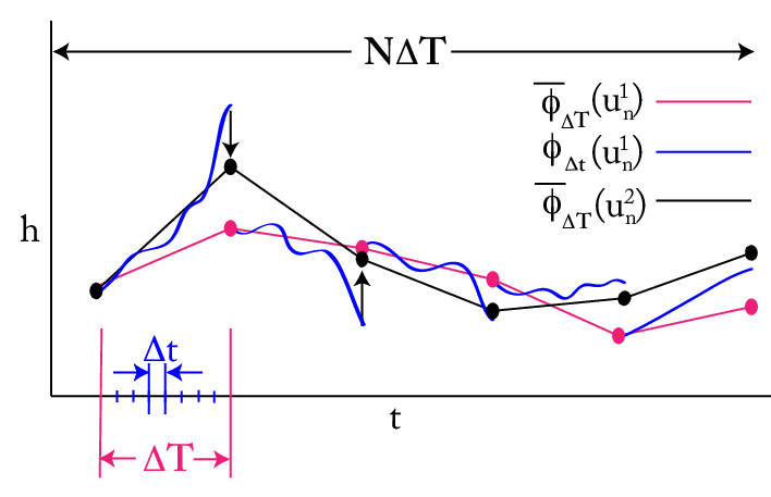
Full pseudocode for the asymptotic parareal method is presented below. In the pseudocode, we use the mid-point rule in the HMM-type scheme for the slow integrator, and Strang splitting for the fine integrator. We assume that $\varphi_{\Delta T}\left(\mathbf{u}_{0}\right)$ is computed using $M$ small time steps $\Delta t$ (so that $\Delta T=M\Delta t$), and that $\overline{\varphi}_{\Delta T}\left(\mathbf{u}_{0}\right)$ is computed using one big time step $\Delta T$.

In geophysical fluid problems, it is often the case that the time scale separation can change in space and time, and it is important that this algorithm works even when there is no scale separation. We give a heauristic derivation of the time average (2.2) from a different point of view, which indicates that the coarse solution yields accuracy even when $\epsilon=\mathcal{O}\left(1\right)$, as long as the time average in (2.2) is performed over a time scale on which the dynamics of the slow nonlinear terms are occurring. Figure 4.1 schematically depicts how the large time step $\Delta T$ varies as a function of the scale separation parameter $\epsilon$, for the asymptotic parareal method, the standard parareal method, and a typical time-stepping method that is used in serial.

As in the integrating factor method, we first factor out the fast oscillatory part,

so that $\mathbf{v}\left(t\right)$ satisfies

Since

$\mathbf{v}\left(t\right)$ varies more slowly than $\mathbf{u}\left(t\right)$ and thus time steps $\Delta T\gg\epsilon$ can potentially be used to solve for $\mathbf{v}\left(t\right)$. However, simply using a standard time-stepping scheme for $\mathbf{v}\left(t\right)$ will still require small step sizes. In fact, differentiating the equation (4.1) shows that $\mathbf{v}\left(t\right)$ has small but rapid fluctuations,

and standard time-stepping schemes will not be accurate unless $\Delta T$ is small.

The idea (see also [3] and [33]) is to take a time step using a smoothed out version of the derivative; this is accomplished by using a moving time average, so that the small $\mathcal{O}\left(\epsilon\right)$ fluctuations in the derivative are removed; see Figure 4.2 for a schematic depiction. In particular, we average the derivative out over a time scale $\epsilon T_{0}$ on which the slow dynamics occur (that is, we average over $T_{0}$ fast oscillations). Then using e.g. forward Euler we get the approximation

where

This approximation allows error control via two different mechanisms. First, when $\epsilon\ll 1$ the above approximation is also an asymptotic approximation, and the time average serves to eliminate secular terms that arise from nonlinear resonances as long as $\Delta T\gg\epsilon$. However, when $\epsilon=\mathcal{O}\left(1\right)$, then we can take $\epsilon T_{0}=\Delta T$ , so that the time average is performed over a scale $\Delta T$ on which the dynamics is slow. In this case, we see that the above approximation is essentially the forward Euler method. In fact, in this case the derivatives of $\mathbf{v}\left(s\right)$ are slow on an $\mathcal{O}\left(\Delta T\right)$ time scale, and we can Taylor expand to get

For systems of ODEs, rigorous error bounds for this “partial time averaging” are derived in Section $3.2$ of [34].

We first discuss the complexity of our algorithm. Although this analysis is standard for the parareal method, the complexity bounds demonstrate (in theory) arbitrarily large parallel speedup as the parameter $\epsilon$ gets smaller. We assume that the time interval $\left[0,1\right]$ is divided into $N$ sub-intervals $\left[T_{n-1},T_{n}\right]$ of length $\Delta T=T_{n}-T_{n-1}=1/N$. We also assume that, within each subinterval, $M$ time steps of size $\Delta t$ are needed for the fine integrator, so that $M=\Delta T/\Delta t$. We let $\tau_{\text{c}}$ denote the (wall-clock) time of computing the coarse solution, $\overline{\varphi}_{\Delta T}\left(\mathbf{u}_{0}\right)$, over a large time step $\Delta T$. Similarly, we let $\tau_{\text{f}}$ denote the (wall-clock) time of computing the fine solution, $\varphi_{\Delta t}\left(\mathbf{u}_{0}\right)$, over a small time step $\Delta t$.

To obtain an initial guess for the parareal method, we first compute the slow approximations $\mathbf{U}_{n}^{0}=\overline{\varphi}_{\Delta T}\left(\mathbf{U}_{n-1}^{0}\right)$, $n=1,\ldots,N$, which takes a wall-clock time of $\tau_{c}N$. Next, suppose that we are at a given iteration level $k$, and we need to compute the next iterations $\mathbf{U}_{n}^{k+1}$ from $\mathbf{U}_{n}^{k}$. To do so, we first need to compute, in parallel, the difference $\mathbf{V}_{n}^{k}=\varphi_{\Delta T}\left(\mathbf{U}_{n}^{k}\right)-\overline{\varphi}_{\Delta T}\left(\mathbf{U}_{n}^{k}\right)$ between the coarse and fine solutions. This takes a wall-clock time of $\tau_{\text{c}}+\tau_{\text{f}}M$. We then need to compute, in serial, the updated approximations $\mathbf{U}_{n}^{k+1}=\overline{\varphi}_{\Delta T_{n-1}}\left(\mathbf{U}_{n-1}^{k+1}\right)+\mathbf{V}_{n-1}^{k},\,\,\,\,n=1,\ldots,N-1$. This takes a wall-clock time of $\tau_{\text{c}}N$, for an overall cost of $\tau_{\text{f}}M+\tau_{\text{c}}N+\tau_{\text{c}}$ per iteration. Thus, after $\nu$ iterations, the overall cost of the parareal method is $\nu\left(\tau_{\text{f}}M+\tau_{\text{c}}N+\tau_{\text{c}}\right)+\tau_{\text{c}}N$. In contrast, directly solving (1.1) in serial requires time $\tau_{\text{f}}NM$. Thus, the estimated parallel speedup is

Notice that an upper bound on the speedup is proportional to $M=\Delta T/\Delta t$, the ratio of slow to fine time step sizes.

In order for the asymptotic parareal method to converge, the fine solver needs time steps $\Delta t$ that are some fraction $a$ of $\epsilon$, $\Delta t=a\epsilon$, where $0<a<1$. Therefore, $\Delta T=M\Delta t=aM\epsilon$, and $NM=\left(N\Delta T/\Delta t\right)=1/\left(a\epsilon\right)$. Now, since

this suggests taking $\tau_{\text{c}}N=\tau_{\text{f}}M$ (this choice also balances the two terms in the upper bound (5.1)). Therefore,

and the estimated parallel speedup is given by

which results in arbitrarily speedup relative to standard numerical integrators.

Recall that computing a time step for the coarse solver, $\overline{\varphi}_{\Delta T}\left(\mathbf{u}_{0}\right)$, requires evaluating the time average (2.1). Since this can be performed in an embarassingly parallel manner, the (wall-clock) time $\tau_{\text{c}}$ satisfies $\tau_{\text{c}}\sim\log_{2}\left(\overline{M}\right)$, where $\overline{M}$ is the number of terms taken in the time average (2.1) (see Algorithm 1). Also, as discussed in Section 2, $\overline{M}\sim\epsilon^{-r}$, where $0<r<1$, and so the estimated parallel speedup scales like $\left(\epsilon\log_{2}\left(\epsilon^{-1}\right)\right)^{-1/2}$. In particular, this results in arbitrarily large efficiency gains relative to standard numerical integrators as $\epsilon\rightarrow 0$. Note that, since $r<1$, arbitrary speedup is also possible without evaluating the time average (2.1) in parallel; however, we have found that this may be necessary for obtaining satisfactory speedup when $\epsilon$ is only moderately small. We remark that evaluating the average in parallel requires more processors, and therefore decrease the parallel efficiency relative to standard parareal (in the experiments in Section 6, evaluating the average in parallel requires about a factor of $1.3$ or less extra processors).

We now use the theory developed in [5] (see also [19]) for our error bounds. As in [5], we consider a scale of Banach spaces $B_{0}\supseteq B_{1}\supseteq B_{2}\supseteq\cdots$, where $B_{j}$ typically quantifies the degree of regularity (i.e., functions in $B_{j+1}$ are more smooth than functions in $B_{j}$). This consideration is useful when obtaining error bounds for infinite-dimensional systems. In fact, as discussed in [5], sufficient regularity constraints can be needed on the initial condition in order to ensure convergence of the parareal method (especially in the absence of numerical or analytical dissipation, and on long time intervals). Also, rigorous bounds between the solution to (1.1), and its asymptotic approximation obtained from (1.2), can require controlling “small denominators” that can arise from near resonances; this can often be achieved if the intial condition is sufficiently smooth. For example, for the so-called primitive equations—which are fundamental in geophysical fluid dynamics—rigorous error bounds for the asymptotic approximation (1.2) have been derived in [32]. These bounds demonstrate that the error in the asymptotic approximation is small, as long as the initial condition is sufficiently smooth.

In order to account for the error that arises from solving the slow evolution equation (1.2) numerically with a time-stepping algorithm, we first need to introduce some more notation. In particular, let $\widetilde{\varphi}_{\Delta T}\left(\mathbf{u}_{0}\right)$ denote the evolution operator associated with solving the slow equation (1.2) using an order $p$ time-stepping method, so that $\widetilde{\varphi}_{\Delta T}\left(\mathbf{u}_{0}\right)$ is a numerical approximation to $\overline{\varphi}_{\Delta T}\left(\mathbf{u}_{0}\right)$. We derive error bounds for the iteration

Notice that, in contrast to the iteration (3.1) presented in Section 3, we explicitly include the numerical approximation $\widetilde{\varphi}_{\Delta T}\left(\mathbf{U}_{n-1}^{k-1}\right)$ to $\overline{\varphi}_{\Delta T}\left(\mathbf{U}_{n-1}^{k-1}\right)$ in the analysis. It is also possible to include the error arising from computing the fine solution $\varphi_{\Delta T}\left(\mathbf{U}_{n-1}^{k-1}\right)$ with a time-stepping scheme, but this requires no additional techniques and is omitted for simplicity.

Define the operators $\mathcal{E}_{\varphi,\overline{\varphi}}\left(\cdot\right)$ and $\mathcal{E}_{\overline{\varphi},\widetilde{\varphi}}\left(\cdot\right)$,

Then following [5], we make the following assumptions on $\varphi_{\Delta T}\left(\cdot\right)$, $\overline{\varphi}_{\Delta T}\left(\cdot\right)$, $\widetilde{\varphi}_{\Delta T}\left(\cdot\right)$, $\mathcal{E}_{\varphi,\overline{\varphi}}\left(\cdot\right)$, and $\mathcal{E}_{\overline{\varphi},\widetilde{\varphi}}\left(\cdot\right)$:

1. (1)

   The operators $\varphi_{t}\left(\cdot\right)$ and $\overline{\varphi}_{t}\left(\cdot\right)$ are uniformly bounded for $0\leq t\leq 1$,

   (5.4)

   $$\left\|\varphi_{t}\left(\mathbf{u}_{0}\right)\right\|_{B_{j}}\leq C_{j}\left\|\mathbf{u}_{0}\right\|_{B_{j+1}},\,\,\,\,\left\|\overline{\varphi}_{t}\left(\mathbf{u}_{0}\right)\right\|_{B_{j}}\leq C_{j}\left\|\mathbf{u}_{0}\right\|_{B_{j+1}}.$$

2. (2)

   The asymptotic approximation is accurate in the sense that

   (5.5)

   $$\left\|\varphi_{t}\left(\mathbf{u}_{0}\right)-\overline{\varphi}_{t}\left(\mathbf{u}_{0}\right)\right\|_{B_{j}}\leq\epsilon C_{j}\left\|\mathbf{u}_{0}\right\|_{B_{j+1}},\,\,\,\,\,0\leq t\leq 1.$$

3. (3)

   The operator $\overline{\varphi}_{\Delta T}\left(\cdot\right)$ satisfies

   (5.6)

   $$\left\|\overline{\varphi}_{\Delta T}\left(\mathbf{u}_{1}\right)-\overline{\varphi}_{\Delta T}\left(\mathbf{u}_{2}\right)\right\|_{B_{j}}\leq\left(1+C_{j}\Delta T\right)\left\|\mathbf{u}_{1}-\mathbf{u}_{2}\right\|_{B_{j}},$$

   and its numerical approximation $\widetilde{\varphi}_{\Delta T}\left(\cdot\right)$ satisfies

   (5.7)

   $$\left\|\widetilde{\varphi}_{\Delta T}\left(\mathbf{u}_{1}\right)-\widetilde{\varphi}_{\Delta T}\left(\mathbf{u}_{2}\right)\right\|_{B_{j}}\leq\left(1+C_{j}\Delta T\right)\left\|\mathbf{u}_{1}-\mathbf{u}_{2}\right\|_{B_{j}}.$$

4. (4)

   The operators $\mathcal{E}_{\varphi,\overline{\varphi}}\left(\cdot\right)$, and $\mathcal{E}_{\overline{\varphi},\widetilde{\varphi}}\left(\cdot\right)$ satisfy

   (5.8)

   $$\left\|\mathcal{E}_{\varphi,\overline{\varphi}}\left(\mathbf{u}_{1}\right)-\mathcal{E}_{\varphi,\overline{\varphi}}\left(\mathbf{u}_{2}\right)\right\|_{B_{j}}\leq\epsilon C_{j}\left\|\mathbf{u}_{1}-\mathbf{u}_{2}\right\|_{B_{j+1}},$$

   and

   (5.9)

   $$\left\|\mathcal{E}_{\overline{\varphi},\widetilde{\varphi}}\left(\mathbf{u}_{1}\right)-\mathcal{E}_{\overline{\varphi},\widetilde{\varphi}}\left(\mathbf{u}_{2}\right)\right\|\leq C_{j}\Delta T^{p+1}\left\|\mathbf{u}_{1}-\mathbf{u}_{2}\right\|_{B_{j+1}}.$$

   for some $p\geq 1$.

Recalling that $T_{n}=n\Delta T$, a slight modification of the proof of Theorem $1$ in [5] immediately yields the convergence result stated below. In particular, taking $\Delta T=\epsilon^{1/2}$, the error scales asymptotically like $\epsilon^{k+1/2}$ after the $k$th iteration (the choice of scaling $\Delta T\sim\epsilon^{1/2}$ yields a speedup that scales like $\epsilon^{-1/2}$).

References

- [1] G. Ariel, B. Engquist, S. Kim, Y. Lee, and R. Tsai. A multiscale method for highly oscillatory dynamical systems using a poincaré map type technique. Journal of Scientific Computing, 54:247–268, 2013.
- [2] Gil Ariel, Bjorn Engquist, and Richard Tsai. A multiscale method for highly oscillatory ordinary differential equations with resonance. Math. Comp., 78(266):929–956, 2009.
- [3] Gil Ariel, Björn Engquist, Heinz-Otto Kreiss, and Richard Tsai. Multiscale computations for highly oscillatory problems. In Björn Engquist, Per Lötstedt, and Olof Runborg, editors, Multiscale Modeling and Simulation in Science, volume 66 of Lecture Notes in Computational Science and Engineering, pages 237–287. Springer Berlin Heidelberg, 2009.
- [4] L. Baffico, S. Bernard, Y. Maday, G. Turinici, and G. Zérah. Parallel-in-time molecular-dynamics simulations. Phys. Rev. E, 66:057701, Nov 2002.
- [5] Guillaume Bal. On the convergence and the stability of the parareal algorithm to solve partial differential equations. In Domain Decomposition Methods in Science and Engineering, volume 40 of Lecture Notes in Computational Science and Engineering, pages 425–432. Springer Berlin Heidelberg, 2005.
- [6] F. Castella, P. Chartier, and E. Faou. An averaging technique for highly oscillatory Hamiltonian problems. SIAM J. Numer. Anal., 47(4):2808–2837, 2009.
- [7] J.G. Charney. On the scale of atmospheric motions. Geofysiske Publikasjoner, 17(2):3–17, 1948.
- [8] J.G. Charney. On a physical basis for numerical prediction of large-scale motions in the atmosphere. Journal of Meterology, 6:371–385, 1949.
- [9] S.M. Cox and P.C. Matthews. Exponential time differencing for stiff systems. Journal of Computational Physics, 176(2):430 – 455, 2002.
- [10] X. Dai and Y. Maday. Stable parareal in time method for first- and second-order hyperbolic systems. SIAM Journal on Scientific Computing, 35(1):A52–A78, 2013.
- [11] Weinan E. Analysis of the heterogeneous multiscale method for ordinary differential equations. Commun. Math. Sci., 1(3):423–436, 2003.
- [12] Weinan E and Bjorn Engquist. Multiscale modeling and computation. Notices Amer. Math. Soc, 50(50):1062–1070, 2003.
- [13] Weinan E, Bjorn Engquist, Xiantao Li, Weiqing Ren, and Eric Vanden-Eijnden. Heterogeneous multiscale methods: A review. Communications in Computational Physics, 2(3):367–450, June 2007.
- [14] S. Engblom. Parallel in time simulation of multiscale stochastic chemical kinetics. Multiscale Modeling and Simulation, 8(1):46–68, 2009.
- [15] Bjorn Engquist and Yen-Hsi Tsai. Heterogeneous multiscale methods for stiff ordinary differential equations. Mathematics of Computation, 74(252):pp. 1707–1742, 2005.
- [16] Charbel Farhat and Marion Chandesris. Time-decomposed parallel time-integrators: theory and feasibility studies for fluid, structure, and fluid?structure applications. International Journal for Numerical Methods in Engineering, 58(9):1397–1434, 2003.
- [17] Paul F. Fischer, Frédéric Hecht, and Yvon Maday. A parareal in time semi-implicit approximation of the navier-stokes equations. In Proceedings of Fifteen International Conference on Domain Decomposition Methods, pages 433–440. Springer Verlag, 2004.
- [18] Martin J. Gander. Analysis of the parareal algorithm applied to hyperbolic problems using characteristics. Bol. Soc. Esp. Mat. Apl. SMA, (42):21–35, 2008.
- [19] MartinJ. Gander and Ernst Hairer. Nonlinear convergence analysis for the parareal algorithm. In Ulrich Langer, Marco Discacciati, DavidE. Keyes, OlofB. Widlund, and Walter Zulehner, editors, Domain Decomposition Methods in Science and Engineering XVII, volume 60 of Lecture Notes in Computational Science and Engineering, pages 45–56. Springer Berlin Heidelberg, 2008.
- [20] Ernst Hairer, Christian Lubich, and Gerhard Wanner. Geometric numerical integration, volume 31 of Springer Series in Computational Mathematics. Springer, Heidelberg, 2010. Structure-preserving algorithms for ordinary differential equations, Reprint of the second (2006) edition.
- [21] D.a. Jones, a. Mahalov, and B. Nicolaenko. A Numerical Study of an Operator Splitting Method for Rotating Flows with Large Ageostrophic Initial Data. Theoretical and Computational Fluid Dynamics, 13(2):143, 1999.
- [22] Aly khan Kassam, Lloyd, and N. Trefethen. Fourth-order time stepping for stiff pdes. SIAM J. Sci. Comput, 26:1214–1233, 2005.
- [23] J. Douglas Lawson. Generalized runge-kutta processes for stable systems with large lipschitz constants. SIAM Journal on Numerical Analysis, 4(3):pp. 372–380, 1967.
- [24] F. Legoll, T. Lelievre, and G. Samaey. A micro-macro parareal algorithm: application to singularly perturbed ordinary differential equations. ArXiv e-prints, April 2012.
- [25] Frédéric Legoll, Xiaoying Dai, Claude Le Bris, and Yvon Maday. Symmetric parareal algorithms for Hamiltonian systems. ESAIM: Mathematical Modelling and Numerical Analysis, pages 1–56, September 2012.
- [26] Jacques-Louis Lions, Yvon Maday, and Gabriel Turinici. Résolution d’{EDP} par un schéma en temps “pararéel”. C. R. Acad. Sci. Paris Sér. I Math., 332(7):661–668, 2001.
- [27] Yvon Maday. Parareal in time algorithm for kinetic systems based on model reduction. In High-dimensional partial differential equations in science and engineering, volume 41 of CRM Proc. Lecture Notes, pages 183–194. Amer. Math. Soc., Providence, RI, 2007.
- [28] Yvon Maday and Gabriel Turinici. Parallel in time algorithms for quantum control: Parareal time discretization scheme. International Journal of Quantum Chemistry, 93(3):223–228, 2003.
- [29] Andrew Majda. Introduction to {PDE}s and waves for the atmosphere and ocean, volume 9 of Courant Lecture Notes in Mathematics. New York University Courant Institute of Mathematical Sciences, New York, 2003.
- [30] Andrew J. Majda and Pedro Embid. Averaging over Fast Gravity Waves for Geophysical Flows with Unbalanced Initial Data. Theoretical and Computational Fluid Dynamics, 11(3-4):155–169, June 1998.
- [31] B Nadiga, Matthew Hecht, L Margolin, and Piotr Smolarkiewicz. On simulating flows with multiple time scales using a method of averages. Theoretical and Computational Fluid Dynamics, 9(3-4):281–292, 1997.
- [32] M. Petcu, R. Temam, and D. Wirosoetisno. Renormalization group method applied to the primitive equations. J. Differential Equations, 208(1):215–257, 2005.
- [33] Sebastian Reich. Smoothed dynamics of highly oscillatory Hamiltonian systems, December 1995.
- [34] J. A. Sanders and F. Verhulst. Averaging methods in nonlinear dynamical systems / J.A. Sanders, F. Verhulst. Springer-Verlag, New York:, 1985.
- [35] S. Schochet. Fast singular limits of hyperbolic pde’s. Journal of Differential Equations, 114:476–512, 1994.
- [36] Leslie M. Smith and Youngsuk Lee. On near resonances and symmetry breaking in forced rotating flows at moderate Rossby number. Journal of Fluid Mechanics, 535(2005):111–142, July 2005.
- [37] G. A. Staff. The parareal algorithm. a survey of present work. Technical report, Norwegian University of Science and Technology, Dept. of Math. Sciences, 2003.
- [38] Beth a. Wingate, Pedro Embid, Miranda Holmes-Cerfon, and Mark a. Taylor. Low Rossby limiting dynamics for stably stratified flow with finite Froude number. Journal of Fluid Mechanics, 676(2011):546–571, April 2011.