跳到论文正文
W Papers独立论文阅读器 arXiv:1303.6605 论文正文 计算阅读时间 · 0%
引用这篇论文根据当前论文元数据生成,正式投稿前建议核对。


License: arXiv.org perpetual non-exclusive license
arXiv:1303.6605v4 [hep-th] 14 Jan 2015

MADCAP-13-06                              UCLA/13/TEP/102 Color-Kinematics Duality for Pure Yang-Mills and Gravity at One and Two Loops

Zvi Berna, Scott Daviesa, Tristan Dennenb, Yu-tin Huangc, and Josh Nohlea Affiliation: aa Department of Physics and Astronomy, University of California at Los Angeles
Los Angeles, CA 90095-1547, USA

bb Niels Bohr International Academy and Discovery Center
The Niels Bohr Institute
Blegdamsvej 17, DK-2100 Copenhagen, Denmark

cc Michigan Center for Theoretical Physics
Randall Laboratory of Physics
University of Michigan, Ann Arbor, MI 48109, USA
Abstract

We provide evidence in favor of the conjectured duality between color and kinematics for the case of nonsupersymmetric pure Yang-Mills amplitudes by constructing a form of the one-loop four-point amplitude of this theory that makes the duality manifest. Our construction is valid in any dimension. We also describe a duality-satisfying representation for the two-loop four-point amplitude with identical four-dimensional external helicities. We use these results to obtain corresponding gravity integrands for a theory containing a graviton, dilaton, and antisymmetric tensor, simply by replacing color factors with specified diagram numerators. Using this, we give explicit forms of ultraviolet divergences at one loop in four, six, and eight dimensions, and at two loops in four dimensions.

I Introduction

Recent years have seen remarkable progress in computing and understanding scattering processes in gauge and gravity theories, both for phenomenological and theoretical applications. (For various reviews see Refs. [1, 2].) In particular, various new structures have been uncovered in the amplitudes of these theories (see, for example, Ref. [3]). One such structure is the duality between color and kinematics found by Carrasco, Johansson, and one of the authors [4, 5]. This Bern-Carrasco-Johansson (BCJ) duality is conjectured to hold at all loop orders in Yang-Mills theory and its supersymmetric counterparts. Besides imposing strong constraints on gauge-theory amplitudes, whenever a form of a gauge-theory loop integrand is obtained where the duality is manifest, we obtain corresponding gravity integrands simply by replacing color factors by specified gauge-theory kinematic numerator factors.

The duality between color and kinematics has been confirmed in numerous tree-level studies [6, 7, 8, 9, 10, 11], including the construction of explicit representations for an arbitrary number of external legs [12]. At loop level, the duality remains a conjecture, but there is already significant nontrivial evidence in its favor for supersymmetric theories [5, 13, 14, 15, 16, 17] and for special helicity configurations in nonsupersymmetric pure Yang-Mills theory [5, 18]. Here we provide further evidence in favor of the duality at loop level, explicitly showing that it holds for pure Yang-Mills one-loop four-point amplitudes for all polarization states in DD dimensions. We also present a duality-satisfying representation of the two-loop four-point identical-helicity amplitude of pure Yang-Mills. This amplitude in a non-duality-satisfying representation was first given in Ref. [19], while Ref. [5] noted the existence of a duality-satisfying form. Here we explicitly give the full duality-satisfying form, including contributions from diagrams absent from Ref. [19] that vanish under integration but are necessary to make the duality manifest.

In order to construct the one-loop four-point pure Yang-Mills amplitude, we use a DD-dimensional variant [20] of the unitarity method [21]. Our construction begins by finding an ansatz for the amplitude constrained to satisfy the duality. Since the amplitude is fully determined from its DD-dimensional unitarity cuts, we obtain a form of the amplitude with the duality manifest by enforcing that the ansatz has the correct unitarity cuts. The existence of such a form where both the duality and the cuts are simultaneously satisfied is rather nontrivial. We do not use helicity states tied to specific dimensions but instead use formal polarization vectors because we wish to have an expression for the amplitude valid in any dimension and for all states. The price for this generality is that the expressions are lengthier. Since the constructed integrand has manifest BCJ duality, the double-copy construction immediately gives the corresponding gravity amplitude in a theory with a graviton, dilaton, and antisymmetric tensor.

We use these results to study the ultraviolet divergences of the corresponding gravity amplitudes. Recent years have seen a renaissance in the study of ultraviolet divergences in gravity theories, in a large measure due to the greatly improved ability to carry out explicit multiloop computations in gravity theories [22, 5, 14, 15, 13, 23, 24]. The unitarity method also has revealed hints that multiloop supergravity theories may be better behaved in the ultraviolet than power-counting arguments based on standard symmetries suggest [25]. Even pure Einstein gravity at one loop exhibits surprising cancellations as the number of external legs increases [26]. The question of whether it is possible to construct a finite supergravity is still an open one, though there has been enormous progress on this question in recent years, including new computations and a much better understanding of the consequences of supersymmetry and duality symmetry (see e.g. Refs. [27, 28]). In half-maximal supergravity [29], two- and three-loop examples are known where the divergence vanishes, yet the understanding of the possible symmetry behind this vanishing is incomplete [28, 23, 30, 24]. The duality between color and kinematics and its associated double-copy formula offer a new angle on the ultraviolet divergences in supergravity theories [5, 13, 23, 24, 31]. Here we explore the ultraviolet properties of nonsupersymmetric gravity from the double-copy perspective.

We use the gravity integrands constructed via the double-copy property to determine the exact form of the ultraviolet divergences. We do so at one loop in dimensions D=4,6,8D=4,6,8. The ultraviolet properties of one-loop four-point gravity amplitudes have already been studied in some detail over the years, including cases with scalars or antisymmetric tensors coupling to gravity [32, 33, 34, 35, 36, 26], so no surprises should be expected, at least at four points. Nevertheless, it is useful to look in some detail at the ultraviolet properties to understand them from the double-copy perspective. Here we examine the four-point amplitudes in a theory of gravity coupled to a dilaton and an antisymmetric tensor, corresponding to the double copy of pure Yang-Mills theory. While related calculations have been carried out, we are unaware of any calculations of the ultraviolet properties in the theory corresponding to the double-copy theory.

We find that in D=4D=4, there are no one-loop divergences in amplitudes involving external gravitons, though there are divergences in the remaining amplitudes involving only external dilatons or antisymmetric tensors, as expected from simple counterterm arguments [32]. By two loops, even the four-graviton amplitudes contain divergences, as we demonstrate by computing the form and numerical coefficient of the divergence. In the two-loop case, the divergence is proportional to a unique R3R^{3} operator which gives a divergence in the identical-helicity four-point amplitude. This means that the identical-helicity four-point amplitude is sufficient for determining the coefficient of the R3R^{3} divergence. In D=6D=6 and D=8D=8, we find one-loop divergences in the four-external-graviton amplitudes. These results are not surprising and are in line with the earlier studies. Our conclusion is that, by itself, the double-copy structure is insufficient to render a gravity theory finite in D=4D=4 and requires additional ultraviolet cancellations, such as those from supersymmetry.

This paper is organized as follows. In Section II, we briefly review the duality between color and kinematics and the double-copy construction of gravity. In Section III, we present the construction of the duality-satisfying pure Yang-Mills numerators at one and two loops. Then in Section IV, we study the ultraviolet properties of gravity coupled to a dilaton and an antisymmetric tensor at one loop in four, six, and eight dimensions. In the same section, we also present the ultraviolet properties at two loops in four dimensions. Finally, in Section V we give our conclusions. Appendices evaluating two-loop integrals needed in Section IV.2 are included. Appendix A focuses on extracting the divergences in dimensional regularization. This procedure mixes infrared and ultraviolet divergences; so, in Appendix B we give the infrared divergences that must be subtracted to obtain the ultraviolet ones. Appendix C evaluates the integrals using an alternative method for obtaining the ultraviolet divergences more directly, by introducing a mass to separate out the infrared divergences from the ultraviolet ones.

II Review of BCJ Duality

An LL-loop mm-point gauge-theory amplitude in DD dimensions, with all particles in the adjoint representation, may be written as

𝒜mL​-​loop=iL​gm−2+2​L​∑𝒮m∑j∫∏l=1LdD​pl(2​π)D​1Sj​cj​nj∏αjpαj2,\mathcal{A}^{L\hbox{-}\mathrm{loop}}_{m}=i^{L}g^{m-2+2L}\sum_{\mathcal{S}_{m}}\sum_{j}\int\prod_{l=1}^{L}\frac{d^{D}p_{l}}{(2\pi)^{D}}\frac{1}{S_{j}}\frac{c_{j}n_{j}}{\prod_{\alpha_{j}}p^{2}_{\alpha_{j}}}\,, (1)

where gg is the gauge coupling constant. The first sum runs over the m!m! permutations of the external legs, denoted by 𝒮m\mathcal{S}_{m}. The SjS_{j} symmetry factor removes any overcounting from these permutations and also from any internal automorphism symmetries of graph jj. The jj-sum is over the set of distinct, nonisomorphic, mm-point LL-loop graphs with only cubic (i.e., trivalent) vertices. These graphs are sufficient because any diagram with quartic or higher vertices can be converted to a diagram with only cubic vertices by multiplying and dividing by the appropriate propagators. The propagators appearing in the graph are 1/∏αjpαj21/\prod_{\alpha_{j}}p^{2}_{\alpha_{j}}. The nontrivial kinematic information is contained in the numerators njn_{j} and depends on momenta, polarizations, and spinors. In supersymmetric cases it will depend also on Grassmann parameters, if a superspace form is used. The loop integral is over LL independent DD-dimensional loop momenta, plp_{l}. Finally, cjc_{j} denotes the color factor, obtained by dressing every vertex in graph jj with the group-theory structure constant, f~a​b​c=i​2​fa​b​c=Tr⁡([Ta,Tb]​Tc)\tilde{f}^{abc}=i\sqrt{2}f^{abc}=\mathrm{Tr}([T^{a},T^{b}]T^{c}), where the hermitian generators of the gauge group are normalized via Tr⁡(Ta​Tb)=δa​b.\mathrm{Tr}(T^{a}T^{b})=\delta^{ab}.

Refer to caption
Figure 1: The basic Jacobi relation for either color or numerator factors. These three diagrams can be embedded in a larger diagram, including loops.

The numerators appearing in Eq. (1) are by no means unique because of freedom in moving terms between different diagrams. Utilizing this freedom, the BCJ conjecture is that to all loop orders, representations of the amplitude exist where kinematic numerators obey the same algebraic relations that the color factors obey [4, 5]. In ordinary gauge theories, this is simply the Jacobi identity,

ci=cj−ck⇒ni=nj−nk,c_{i}=c_{j}-c_{k}\ \Rightarrow\ n_{i}=n_{j}-n_{k}\,, (2)

where ii, jj, and kk label three diagrams whose color factors obey the Jacobi identity. The basic Jacobi identity is displayed in Fig. 1. The identity generalizes to any loop order with any number of external legs by embedding it in larger diagrams, where the other parts of the diagrams are identical for the three diagrams. Furthermore, if the color factor of a diagram is antisymmetric under a swap of legs, we require that the numerator obey the same antisymmetry,

ci→−ci⇒ni→−ni.c_{i}\rightarrow-c_{i}\ \Rightarrow\ n_{i}\rightarrow-n_{i}\,. (3)

The duality was noticed long ago for tree-level four-point Feynman diagrams [37]; beyond this, it is rather nontrivial and no longer holds for ordinary Feynman diagrams. We note that the numerator relations are nontrivial functional relations because they depend on momenta, polarizations, and spinors, as discussed in some detail in Refs. [13, 2, 11].

While a complete understanding of the duality and its consequences is still lacking, a variety of studies have elucidated it, especially at tree level. In particular, this duality leads to nontrivial relations between gauge-theory color-ordered partial tree amplitudes [4, 38]. The duality (3) has also been studied in string theory [39, 6, 9]. In the self-dual case, light-cone gauge Feynman rules have been shown to exhibit the duality [10]. Explicit forms of nn-point tree amplitudes satisfying the duality have been found [12]. Although we do not yet have a complete Lagrangian understanding, some progress in this direction can be found in Refs. [8, 10]. The duality (2) does not need to be expressed in terms of group structure constants but can alternatively be expressed in terms of a trace-based representation [40]. Progress has also been made in understanding the underlying infinite-dimensional Lie algebra [10, 41] responsible for the duality. The duality between color and kinematics also appears to hold in three-dimensional theories based on three algebras [42], as well as in some cases with higher-dimension operators [43]. Some initial studies of duality and its implications for gravity in the high-energy limit have also been carried out [44].

At loop level, the duality remains a conjecture, but there is already nontrivial evidence in its favor, especially for supersymmetric theories. At present, the list of loop-level cases where duality-satisfying forms of the amplitude are known to hold includes:

  • •

    Up to four loops for four-point 𝒩=4\mathcal{N}=4 super-Yang-Mills [5, 13] in a form valid in DD dimensions;

  • •

    up to two loops for five external gluons in 𝒩=4\mathcal{N}=4 super-Yang-Mills theory [45];

  • •

    up to seven points for one-loop amplitudes in 𝒩=4\mathcal{N}=4 super-Yang-Mills theory [46];

  • •

    up to two loops for four-point identical-helicity pure Yang-Mills amplitudes [5];

  • •

    through nn points for one-loop all-plus- or single-minus-helicity pure Yang-Mills amplitudes [18];

  • •

    through four loops for a two-point (Sudakov) form factor in 𝒩=4\mathcal{N}=4 super-Yang-Mills theory [47];

  • •

    one-loop four-point amplitudes in Yang-Mills theories with less than maximally supersymmetric amplitudes [17].

In this paper, we add the nonsupersymmetric pure Yang-Mills one-loop four-point amplitude in DD dimensions to this list. Besides direct constructions, we note that the duality also appears to be consistent with loop-level infrared properties of both gauge and gravity theories [16].

Another significant aspect of the duality is the ease with which gravity loop integrands can be obtained from gauge-theory ones, once the duality is made manifest [4, 5]. One simply replaces the color factor with a kinematic numerator from a second gauge theory,

ci→n~i.c_{i}\ \rightarrow\ \tilde{n}_{i}\,. (4)

This immediately gives the double-copy form of gravity amplitudes,

ℳmL​-​loop=iL+1​(κ2)m−2+2​L​∑𝒮m∑j∫∏l=1LdD​pl(2​π)D​1Sj​n~j​nj∏αjpαj2,\mathcal{M}^{L\hbox{-}\mathrm{loop}}_{m}=i^{L+1}\left(\frac{\kappa}{2}\right)^{m-2+2L}\sum_{\mathcal{S}_{m}}\sum_{j}\int\prod_{l=1}^{L}\frac{d^{D}p_{l}}{(2\pi)^{D}}\frac{1}{S_{j}}\frac{\tilde{n}_{j}n_{j}}{\prod_{\alpha_{j}}p^{2}_{\alpha_{j}}}\,, (5)

where n~j\tilde{n}_{j} and njn_{j} are gauge-theory numerator factors. Only one of the two sets of numerators needs to satisfy the duality (2) [5, 8] in order for the double-copy form (5) to be valid. The double-copy formalism has been studied at loop level in some detail in a variety of cases [5, 14, 45, 13, 23, 24, 16, 46].

III Construction of Duality-Satisfying Integrands

We now describe the construction of a duality-satisfying representation of the one-loop four-point amplitude in pure Yang-Mills. Since we want the form to be valid in all dimensions and for all D−2D-2 gluon states, we use formal polarizations instead of helicity states. This complicates the expression for the amplitude, but has the advantage that it allows us to straightforwardly study the amplitude and its gravity double copy in various dimensions. In this section, we also present a form of the two-loop pure Yang-Mills identical-helicity amplitude given in Ref. [19] that satisfies BCJ duality after some rearrangement and addition of diagrams that integrate to zero. In Section IV.2, we use this amplitude to show that although four-graviton amplitudes are ultraviolet finite in D=4D=4 at one loop, they diverge at two loops, in accordance with expectations.

III.1 One Loop

Refer to caption
Figure 2: The Jacobi relations determining either color or kinematic numerators of the four-point diagrams containing either a triangle or internal bubble.
Refer to caption
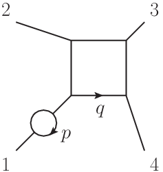
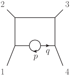
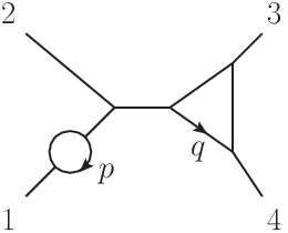
Figure 3: The color or kinematic Jacobi relations involving a bubble on an external leg or a tadpole. These diagrams have vanishing contribution to the integrated amplitude.

For a one-loop nn-point amplitude, the duality (2) can be used to express kinematic numerators of any diagram directly in terms of nn-gon numerators. In particular, for the four-point case we have two basic relations determining triangle and bubble contributions from box numerators as illustrated in Fig. 2,

n12​(34);p\displaystyle n_{12(34);p} =\displaystyle= n1234;p−n1243;p,\displaystyle n_{1234;p}-n_{1243;p}\,,
n(12)​(34);p\displaystyle n_{(12)(34);p} =\displaystyle= n12​(34);p−n21​(34);p.\displaystyle n_{12(34);p}-n_{21(34);p}\,. (6)

The labels 1,2,3,41,2,3,4 refer to the momenta and states of each external leg, while the label pp denotes the loop momentum of the leg indicated in Fig. 2. (The parentheses in the subscript of the numerators indicate which external legs are pinched off to form a tree attached to the loop.) Note that in the figure the momentum of each internal leg of each diagram is the same as in the other two diagrams except for the single internal leg that differs between the diagrams. In general, the bubble and triangle contributions are nonvanishing; indeed, this explicitly holds for the BCJ representation of the one-loop four-point amplitude of pure Yang-Mills theory that we construct.

Besides the diagrams in Fig. 2, there are diagrams with a bubble on an external leg and diagrams with a tadpole, as shown in Fig. 3. The duality also determines the numerators of these diagrams via

n1​(234);p\displaystyle n_{1(234);p} =\displaystyle= n12​(34);p+n1​(43)​2;p,\displaystyle n_{12(34);p}+n_{1(43)2;p}\,,
n(1234);p\displaystyle n_{(1234);p} =\displaystyle= n(12)​(34);p−n(12)​(34);−p,\displaystyle n_{(12)(34);p}-n_{(12)(34);-p}\,,
n(1^​234);p\displaystyle n_{(\hat{1}234);p} =\displaystyle= n1​(234);p−n1​(234);−p,\displaystyle n_{1(234);p}-n_{1(234);-p}\,, (7)

corresponding respectively to the three relations in Fig. 3. (On the final line in Eq. (7), the hat marks leg 1 as the location where the tadpole is attached.) We use these equations to impose the auxiliary constraint that the tadpole numerators determined by BCJ duality vanish identically and that all terms in the bubble-on-external-leg diagrams integrate to zero as they do for Feynman diagrams. Thus, these diagrams are not necessary for determining the integrated amplitudes (though in D=4D=4 the bubble-on-external-leg diagrams do affect the Yang-Mills ultraviolet divergence).

Once we impose the BCJ conditions, the amplitude is entirely specified by the box numerators. Our task is then to find an expression for the box numerators such that we obtain the correct amplitude. It is useful to impose a few auxiliary constraints to help simplify the one-loop construction:

  1. 1.

    The box diagrams should have no more than four powers of loop momenta in the pure Yang-Mills case, matching the usual power count of Feynman-gauge Feynman diagrams.

  2. 2.

    Each numerator written in terms of formal polarization vectors respects the symmetries of the diagrams. In particular, this condition implies that once a box diagram with one ordering of external legs is specified, the other orderings are obtained simply by relabeling.

  3. 3.

    The numerators of tadpole diagrams vanish prior to integration.

  4. 4.

    All terms in the bubble-on-external-leg diagrams integrate to zero, as they do for Feynman diagrams.

While it is not necessary to impose these conditions, they greatly simplify the construction. They ensure that the type of terms that appear in the ansatz are similar to those of ordinary Feynman-gauge Feynman diagrams, avoiding unnecessarily complicated terms. (Using generalized gauge invariance, one can always introduce arbitrarily complicated terms into amplitudes, which cancel at the end.)

The first three conditions simplify the construction by restricting the number of terms that appear. The purpose of the fourth auxiliary constraint is a bit more subtle. While bubble-on-external-leg Feynman diagrams are well defined in the on-shell limit, the freedom to reassign terms used in the construction of BCJ numerators can introduce ill-defined terms into such diagrams. As a simple example, consider the effect of the term (k1+k2)2​ε1⋅k2​ε2⋅k1​ε3⋅ε4(k_{1}+k_{2})^{2}\varepsilon_{1}\cdot k_{2}\varepsilon_{2}\cdot k_{1}\varepsilon_{3}\cdot\varepsilon_{4} when added to the numerator of the first diagram of Fig. 3 (with kik_{i} and εi\varepsilon_{i} external momenta and polarizations). Even after integration, this contribution to the diagram is ill-defined because of the on-shell intermediate propagator. Such singular contributions would need to be regularized by an appropriate off-shell continuation to ensure that the introduced singularities cancel properly against singularities of other diagrams. While in principle we can introduce such a regulator, it is best to avoid this complication altogether. The fourth condition ensures that we can treat the bubble-on-external-leg contributions in the same way as for Feynman diagrams. In particular, with the constraint imposed, the bubble-on-external-leg contributions match the Feynman-diagram property that they are proportional to (ki2)(D−4)/2(k_{i}^{2})^{(D-4)/2}, after accounting for the intermediate on-shell propagator, and hence vanish in D>4D>4, for kik_{i} on shell. We note that even with the fourth constraint, near D=4D=4 we encounter the same subtlety encountered with Feynman diagrams: Although bubble-on-external-leg contributions are set to zero in dimensional regularization, they can carry ultraviolet divergences. Such ultraviolet divergences cancel against infrared ones leaving a vanishing result for on-shell bubble-on-external-leg diagrams. The net effect is that in gauge theory, we need to account for such contributions to obtain the correct ultraviolet divergences. In contrast, in gravity even near D=4D=4 there are neither infrared nor ultraviolet divergences hiding in the bubble-on-external-leg contributions because an extra two powers of numerator momenta give rise to an additional vanishing.

We start the construction with an ansatz containing all possible products of εi⋅εj\varepsilon_{i}\cdot\varepsilon_{j}, p⋅εip\cdot\varepsilon_{i}, ki⋅εjk_{i}\cdot\varepsilon_{j}, p⋅kip\cdot k_{i}, p⋅pp\cdot p, ss, and tt, where the kik_{i} are three independent external momenta, pp is the loop momentum, εi\varepsilon_{i} are external polarization vectors, and

s=(k1+k2)2,t=(k2+k3)2,s=(k_{1}+k_{2})^{2}\,,\hskip 42.67912ptt=(k_{2}+k_{3})^{2}\,, (8)

are the usual Mandelstam invariants. By dimensional analysis, each numerator term must contain four momenta in addition to being linear in all four εi\varepsilon_{i}’s. We also set ki⋅εi=0k_{i}\cdot\varepsilon_{i}=0 and impose momentum conservation with k4=−k1−k2−k3k_{4}=-k_{1}-k_{2}-k_{3} and k1⋅ε4=−k2⋅ε4−k3⋅ε4k_{1}\cdot\varepsilon_{4}=-k_{2}\cdot\varepsilon_{4}-k_{3}\cdot\varepsilon_{4}. This yields 468 terms, each with a coefficient to be determined.

Our first constraint on the coefficients comes from demanding that the box numerator obey the rotation and reflection symmetries of the box diagram. This leaves us with 81 free coefficients. An ansatz for the full amplitude is then obtained by using the duality relations (6), (7) to determine numerators for all other diagrams.

Refer to caption
Refer to caption
Refer to caption
Refer to caption
Refer to caption
Refer to caption
Refer to caption
Figure 4: The seven diagrams for the color-ordered amplitude with ordering (1,2,3,4)(1,2,3,4).
Refer to caption
Refer to caption
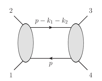
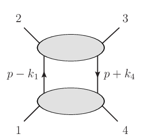
Figure 5: The (a) ss-channel and (b) tt-channel unitarity cuts used to determine the amplitude. The exposed intermediate legs are on shell.

The next step is to determine coefficients in the ansatz by matching to the unitarity cuts of the amplitude. It is convenient to use a color-ordered form of the amplitude [48] for this matching. The seven diagrams contributing to the color-ordered amplitude, that is the coefficient of the color trace Nc​Tr​[Ta1​Ta2​Ta3​Ta4]N_{c}{\rm Tr}[T^{a_{1}}T^{a_{2}}T^{a_{3}}T^{a_{4}}], are shown in Fig. 4. The other color-ordered amplitudes are simple relabelings of this one. For the one-loop four-point amplitude, the ss- and tt-channel unitarity cuts—shown in Fig. 5—are sufficient to determine this color-ordered amplitude up to terms that integrate to zero. One straightforward means for determining the cuts is to construct the amplitude in Feynman gauge and then take its unitarity cuts at the integrand level prior to integration. This automatically gives us an expression for the cuts valid in DD dimensions without any spurious denominators (such as light-cone denominators from physical state projectors). This matching procedure nontrivially rearranges the amplitude so that BCJ duality is manifest. After matching the cuts, we also impose the fourth auxiliary condition to tame the bubble-on-external-leg contributions. Finally we impose that the tadpole numerators vanish. Including all the auxiliary constraints with these conditions, we can solve for all but five free coefficients. Because the ss- and tt-channel unitarity cuts are independent of these parameters, the integrated amplitude should not depend on them.

Using the shorthand notation,

p1=p,p2=p−k1,p3=p−k1−k2,p4=p+k4,\displaystyle p_{1}=p\,,\hskip 28.45274ptp_{2}=p-k_{1}\,,\hskip 28.45274ptp_{3}=p-k_{1}-k_{2}\,,\hskip 28.45274ptp_{4}=p+k_{4}\,,
ℰi​j=εi⋅εj,𝒫i​j=pi⋅εj,𝒦i​j=ki⋅εj,\displaystyle{\cal E}_{ij}=\varepsilon_{i}\cdot\varepsilon_{j}\,,\hskip 56.9055pt{\cal P}_{ij}=p_{i}\cdot\varepsilon_{j}\,,\hskip 56.9055pt{\cal K}_{ij}=k_{i}\cdot\varepsilon_{j}\,, (9)

and setting the free parameters to zero for simplicity, the box numerator is

n1234;p=−i[Ds−28ℰ14ℰ23p12p32+Ds−224ℰ13ℰ24p12p32−Ds−224ℰ12ℰ34p12p32−23ℰ14ℰ23p32s\displaystyle\hskip-14.22636ptn_{1234;p}\>=-i\Bigl[\tfrac{D_{s}-2}{8}\>{\cal E}_{14}\>{\cal E}_{23}\>p_{1}^{2}\>p_{3}^{2}+\tfrac{D_{s}-2}{24}\>{\cal E}_{13}\>{\cal E}_{24}\>p_{1}^{2}\>p_{3}^{2}-\tfrac{D_{s}-2}{24}\>{\cal E}_{12}\>{\cal E}_{34}\>p_{1}^{2}\>p_{3}^{2}-\tfrac{2}{3}\>{\cal E}_{14}\>{\cal E}_{23}\>p_{3}^{2}\>s
−23​ℰ13​ℰ24​p22​s+23​ℰ12​ℰ34​p22​s+23​ℰ14​ℰ23​p22​s+12​ℰ14​ℰ23​s2+2​ℰ23​𝒦24​𝒦41​p32\displaystyle\hbox{}-\tfrac{2}{3}\>{\cal E}_{13}\>{\cal E}_{24}\>p_{2}^{2}\>s+\tfrac{2}{3}\>{\cal E}_{12}\>{\cal E}_{34}\>p_{2}^{2}\>s+\tfrac{2}{3}\>{\cal E}_{14}\>{\cal E}_{23}\>p_{2}^{2}\>s+\tfrac{1}{2}\>{\cal E}_{14}\>{\cal E}_{23}\>s^{2}+2\>{\cal E}_{23}\>{\cal K}_{24}\>{\cal K}_{41}\>p_{3}^{2}\vskip 5.69046pt
+Ds−7424​ℰ13​𝒦12​𝒦34​p32+Ds−7424​ℰ24​𝒦23​𝒦41​p32−Ds−263​ℰ12​𝒦13​𝒦34​p32\displaystyle\hbox{}+\tfrac{D_{s}-74}{24}\>{\cal E}_{13}\>{\cal K}_{12}\>{\cal K}_{34}\>p_{3}^{2}+\tfrac{D_{s}-74}{24}\>{\cal E}_{24}\>{\cal K}_{23}\>{\cal K}_{41}\>p_{3}^{2}-\tfrac{D_{s}-26}{3}\>{\cal E}_{12}\>{\cal K}_{13}\>{\cal K}_{34}\>p_{3}^{2}\vskip 5.69046pt
−Ds−266​ℰ34​𝒦41​𝒦42​p32−Ds−262​ℰ12​𝒦23​𝒦34​p32−Ds−262​ℰ34​𝒦12​𝒦41​p32\displaystyle\hbox{}-\tfrac{D_{s}-26}{6}\>{\cal E}_{34}\>{\cal K}_{41}\>{\cal K}_{42}\>p_{3}^{2}-\tfrac{D_{s}-26}{2}\>{\cal E}_{12}\>{\cal K}_{23}\>{\cal K}_{34}\>p_{3}^{2}-\tfrac{D_{s}-26}{2}\>{\cal E}_{34}\>{\cal K}_{12}\>{\cal K}_{41}\>p_{3}^{2}\vskip 5.69046pt
+Ds−2612​ℰ34​𝒦31​𝒦42​p32+5​(Ds−26)24​ℰ24​𝒦13​𝒦41​p32−Ds−268​ℰ24​𝒦13​𝒦31​p32\displaystyle\hbox{}+\tfrac{D_{s}-26}{12}\>{\cal E}_{34}\>{\cal K}_{31}\>{\cal K}_{42}\>p_{3}^{2}+\tfrac{5(D_{s}-26)}{24}\>{\cal E}_{24}\>{\cal K}_{13}\>{\cal K}_{41}\>p_{3}^{2}-\tfrac{D_{s}-26}{8}\>{\cal E}_{24}\>{\cal K}_{13}\>{\cal K}_{31}\>p_{3}^{2}\vskip 5.69046pt
−11​(Ds−26)24​ℰ24​𝒦23​𝒦31​p32−Ds−2624​ℰ34​𝒦12​𝒦31​p32+Ds−302​ℰ13​𝒦12​𝒦24​p32\displaystyle\hbox{}-\tfrac{11(D_{s}-26)}{24}\>{\cal E}_{24}\>{\cal K}_{23}\>{\cal K}_{31}\>p_{3}^{2}-\tfrac{D_{s}-26}{24}\>{\cal E}_{34}\>{\cal K}_{12}\>{\cal K}_{31}\>p_{3}^{2}+\tfrac{D_{s}-30}{2}\>{\cal E}_{13}\>{\cal K}_{12}\>{\cal K}_{24}\>p_{3}^{2}\vskip 5.69046pt
−Ds−146​ℰ13​𝒦34​𝒦42​p32+Ds−386​ℰ13​𝒦24​𝒦42​p32−5​(Ds−26)24​ℰ12​𝒦13​𝒦24​p32\displaystyle\hbox{}-\tfrac{D_{s}-14}{6}\>{\cal E}_{13}\>{\cal K}_{34}\>{\cal K}_{42}\>p_{3}^{2}+\tfrac{D_{s}-38}{6}\>{\cal E}_{13}\>{\cal K}_{24}\>{\cal K}_{42}\>p_{3}^{2}-\tfrac{5(D_{s}-26)}{24}\>{\cal E}_{12}\>{\cal K}_{13}\>{\cal K}_{24}\>p_{3}^{2}\vskip 5.69046pt
−11​(Ds−26)24​ℰ12​𝒦23​𝒦24​p32+13​Ds−29024​ℰ14​𝒦23​𝒦42​p32+(Ds−24)​ℰ14​𝒦12​𝒦23​p32\displaystyle\hbox{}-\tfrac{11(D_{s}-26)}{24}\>{\cal E}_{12}\>{\cal K}_{23}\>{\cal K}_{24}\>p_{3}^{2}+\tfrac{13D_{s}-290}{24}\>{\cal E}_{14}\>{\cal K}_{23}\>{\cal K}_{42}\>p_{3}^{2}+(D_{s}\!-\!24)\>{\cal E}_{14}\>{\cal K}_{12}\>{\cal K}_{23}\>p_{3}^{2}\vskip 5.69046pt
+11​(Ds−26)24​ℰ14​𝒦13​𝒦42​p32+11​(Ds−26)24​ℰ14​𝒦12​𝒦13​p32−Ds−2612​ℰ23​𝒦24​𝒦31​p32\displaystyle\hbox{}+\tfrac{11(D_{s}-26)}{24}\>{\cal E}_{14}\>{\cal K}_{13}\>{\cal K}_{42}\>p_{3}^{2}+\tfrac{11(D_{s}-26)}{24}\>{\cal E}_{14}\>{\cal K}_{12}\>{\cal K}_{13}\>p_{3}^{2}-\tfrac{D_{s}-26}{12}\>{\cal E}_{23}\>{\cal K}_{24}\>{\cal K}_{31}\>p_{3}^{2}\vskip 5.69046pt
−Ds−2612​ℰ23​𝒦31​𝒦34​p32−Ds−5012​ℰ23​𝒦34​𝒦41​p32−4​ℰ14​𝒦12​𝒦23​s−2​ℰ23​𝒦24​𝒦31​s\displaystyle\hbox{}-\tfrac{D_{s}-26}{12}\>{\cal E}_{23}\>{\cal K}_{31}\>{\cal K}_{34}\>p_{3}^{2}-\tfrac{D_{s}-50}{12}\>{\cal E}_{23}\>{\cal K}_{34}\>{\cal K}_{41}\>p_{3}^{2}-4\>{\cal E}_{14}\>{\cal K}_{12}\>{\cal K}_{23}\>s-2\>{\cal E}_{23}\>{\cal K}_{24}\>{\cal K}_{31}\>s\vskip 5.69046pt
−2​ℰ23​𝒦24​𝒦41​s−2​ℰ12​𝒦23​𝒦24​s−2​ℰ14​𝒦12​𝒦13​s−2​ℰ12​𝒦23​𝒦34​s\displaystyle\hbox{}-2\>{\cal E}_{23}\>{\cal K}_{24}\>{\cal K}_{41}\>s-2\>{\cal E}_{12}\>{\cal K}_{23}\>{\cal K}_{24}\>s-2\>{\cal E}_{14}\>{\cal K}_{12}\>{\cal K}_{13}\>s-2\>{\cal E}_{12}\>{\cal K}_{23}\>{\cal K}_{34}\>s\vskip 5.69046pt
+7​Ds−23012​ℰ23​𝒦31​𝒫44​p32+7​Ds−23024​ℰ23​𝒦34​𝒫11​p32+7​Ds−23024​ℰ23​𝒦41​𝒫44​p32\displaystyle\hbox{}+\tfrac{7D_{s}-230}{12}\>{\cal E}_{23}\>{\cal K}_{31}\>{\cal P}_{44}\>p_{3}^{2}+\tfrac{7D_{s}-230}{24}\>{\cal E}_{23}\>{\cal K}_{34}\>{\cal P}_{11}\>p_{3}^{2}+\tfrac{7D_{s}-230}{24}\>{\cal E}_{23}\>{\cal K}_{41}\>{\cal P}_{44}\>p_{3}^{2}\vskip 5.69046pt
+7​Ds−23024​ℰ13​𝒦34​𝒫22​p32+7​Ds−23024​ℰ24​𝒦41​𝒫33​p32−7​(Ds−26)24​ℰ24​𝒦13​𝒫11​p32\displaystyle\hbox{}+\tfrac{7D_{s}-230}{24}\>{\cal E}_{13}\>{\cal K}_{34}\>{\cal P}_{22}\>p_{3}^{2}+\tfrac{7D_{s}-230}{24}\>{\cal E}_{24}\>{\cal K}_{41}\>{\cal P}_{33}\>p_{3}^{2}-\tfrac{7(D_{s}-26)}{24}\>{\cal E}_{24}\>{\cal K}_{13}\>{\cal P}_{11}\>p_{3}^{2}\vskip 5.69046pt
+7​(Ds−26)24​ℰ12​𝒦13​𝒫44​p32−7​Ds−23024​ℰ23​𝒦24​𝒫11​p32−7​Ds−23024​ℰ12​𝒦24​𝒫33​p32\displaystyle\hbox{}+\tfrac{7(D_{s}-26)}{24}\>{\cal E}_{12}\>{\cal K}_{13}\>{\cal P}_{44}\>p_{3}^{2}-\tfrac{7D_{s}-230}{24}\>{\cal E}_{23}\>{\cal K}_{24}\>{\cal P}_{11}\>p_{3}^{2}-\tfrac{7D_{s}-230}{24}\>{\cal E}_{12}\>{\cal K}_{24}\>{\cal P}_{33}\>p_{3}^{2}\vskip 5.69046pt
−7​Ds−23024​ℰ34​𝒦42​𝒫11​p32−11​Ds−23824​ℰ13​𝒦12​𝒫44​p32−11​Ds−23824​ℰ24​𝒦23​𝒫11​p32\displaystyle\hbox{}-\tfrac{7D_{s}-230}{24}\>{\cal E}_{34}\>{\cal K}_{42}\>{\cal P}_{11}\>p_{3}^{2}-\tfrac{11D_{s}-238}{24}\>{\cal E}_{13}\>{\cal K}_{12}\>{\cal P}_{44}\>p_{3}^{2}-\tfrac{11D_{s}-238}{24}\>{\cal E}_{24}\>{\cal K}_{23}\>{\cal P}_{11}\>p_{3}^{2}\vskip 5.69046pt
+2​ℰ12​𝒦23​𝒫44​p32+2​ℰ34​𝒦12​𝒫11​p32−Ds−146​ℰ13​𝒦42​𝒫44​p32−3​(Ds−26)8​ℰ34​𝒦31​𝒫22​p32\displaystyle\hbox{}+2\>{\cal E}_{12}\>{\cal K}_{23}\>{\cal P}_{44}\>p_{3}^{2}+2\>{\cal E}_{34}\>{\cal K}_{12}\>{\cal P}_{11}\>p_{3}^{2}-\tfrac{D_{s}-14}{6}\>{\cal E}_{13}\>{\cal K}_{42}\>{\cal P}_{44}\>p_{3}^{2}-\tfrac{3(D_{s}-26)}{8}\>{\cal E}_{34}\>{\cal K}_{31}\>{\cal P}_{22}\>p_{3}^{2}\vskip 5.69046pt
−3​(Ds−26)8​ℰ24​𝒦31​𝒫33​p32−2​(Ds−29)3​ℰ34​𝒦41​𝒫22​p32−2​(Ds−29)3​ℰ12​𝒦34​𝒫33​p32\displaystyle\hbox{}-\tfrac{3(D_{s}-26)}{8}\>{\cal E}_{24}\>{\cal K}_{31}\>{\cal P}_{33}\>p_{3}^{2}-\tfrac{2(D_{s}-29)}{3}\>{\cal E}_{34}\>{\cal K}_{41}\>{\cal P}_{22}\>p_{3}^{2}-\tfrac{2(D_{s}-29)}{3}\>{\cal E}_{12}\>{\cal K}_{34}\>{\cal P}_{33}\>p_{3}^{2}\vskip 5.69046pt
+13​Ds−29024​ℰ14​𝒦42​𝒫33​p32+13​Ds−29024​ℰ14​𝒦12​𝒫33​p32+13​Ds−29024​ℰ14​𝒦23​𝒫22​p32\displaystyle\hbox{}+\tfrac{13D_{s}-290}{24}\>{\cal E}_{14}\>{\cal K}_{42}\>{\cal P}_{33}\>p_{3}^{2}+\tfrac{13D_{s}-290}{24}\>{\cal E}_{14}\>{\cal K}_{12}\>{\cal P}_{33}\>p_{3}^{2}+\tfrac{13D_{s}-290}{24}\>{\cal E}_{14}\>{\cal K}_{23}\>{\cal P}_{22}\>p_{3}^{2}\vskip 5.69046pt
+2​(Ds−29)3​ℰ13​𝒦24​𝒫22​p32−2​ℰ14​𝒦42​𝒫33​s−2​ℰ34​𝒦41​𝒫22​s−2​ℰ14​𝒦12​𝒫33​s\displaystyle\hbox{}+\tfrac{2(D_{s}-29)}{3}\>{\cal E}_{13}\>{\cal K}_{24}\>{\cal P}_{22}\>p_{3}^{2}-2\>{\cal E}_{14}\>{\cal K}_{42}\>{\cal P}_{33}\>s-2\>{\cal E}_{34}\>{\cal K}_{41}\>{\cal P}_{22}\>s-2\>{\cal E}_{14}\>{\cal K}_{12}\>{\cal P}_{33}\>s\vskip 5.69046pt
−2​ℰ12​𝒦24​𝒫33​s−2​ℰ12​𝒦34​𝒫33​s−2​ℰ14​𝒦23​𝒫22​s+2​ℰ13​𝒦34​𝒫22​s+2​ℰ24​𝒦41​𝒫33​s\displaystyle\hbox{}-2\>{\cal E}_{12}\>{\cal K}_{24}\>{\cal P}_{33}\>s-2\>{\cal E}_{12}\>{\cal K}_{34}\>{\cal P}_{33}\>s-2\>{\cal E}_{14}\>{\cal K}_{23}\>{\cal P}_{22}\>s+2\>{\cal E}_{13}\>{\cal K}_{34}\>{\cal P}_{22}\>s+2\>{\cal E}_{24}\>{\cal K}_{41}\>{\cal P}_{33}\>s\vskip 5.69046pt
+2​ℰ13​𝒦24​𝒫22​s−(Ds−2)​ℰ23​𝒫11​𝒫44​p32−Ds−26​ℰ13​𝒫22​𝒫44​p32−Ds−26​ℰ24​𝒫33​𝒫11​p32\displaystyle\hbox{}+2\>{\cal E}_{13}\>{\cal K}_{24}\>{\cal P}_{22}\>s-(D_{s}\!-\!2)\>{\cal E}_{23}\>{\cal P}_{11}\>{\cal P}_{44}\>p_{3}^{2}-\tfrac{D_{s}-2}{6}\>{\cal E}_{13}\>{\cal P}_{22}\>{\cal P}_{44}\>p_{3}^{2}-\tfrac{D_{s}-2}{6}\>{\cal E}_{24}\>{\cal P}_{33}\>{\cal P}_{11}\>p_{3}^{2}\vskip 5.69046pt
+Ds−26​ℰ12​𝒫33​𝒫44​p32+Ds−26​ℰ34​𝒫11​𝒫22​p32−4​ℰ34​𝒫11​𝒫22​s+2​ℰ13​𝒫22​𝒫44​s\displaystyle\hbox{}+\tfrac{D_{s}-2}{6}\>{\cal E}_{12}\>{\cal P}_{33}\>{\cal P}_{44}\>p_{3}^{2}+\tfrac{D_{s}-2}{6}\>{\cal E}_{34}\>{\cal P}_{11}\>{\cal P}_{22}\>p_{3}^{2}-4\>{\cal E}_{34}\>{\cal P}_{11}\>{\cal P}_{22}\>s+2\>{\cal E}_{13}\>{\cal P}_{22}\>{\cal P}_{44}\>s\vskip 5.69046pt
+2​ℰ24​𝒫33​𝒫11​s+4​𝒦12​𝒦13​𝒦24​𝒦31+4​𝒦12​𝒦23​𝒦24​𝒦31+2​𝒦12​𝒦13​𝒦31​𝒦34\displaystyle\hbox{}+2\>{\cal E}_{24}\>{\cal P}_{33}\>{\cal P}_{11}\>s+4\>{\cal K}_{12}\>{\cal K}_{13}\>{\cal K}_{24}\>{\cal K}_{31}+4\>{\cal K}_{12}\>{\cal K}_{23}\>{\cal K}_{24}\>{\cal K}_{31}+2\>{\cal K}_{12}\>{\cal K}_{13}\>{\cal K}_{31}\>{\cal K}_{34}\vskip 5.69046pt
+4​𝒦12​𝒦23​𝒦31​𝒦34+𝒦13​𝒦24​𝒦31​𝒦42+2​𝒦12​𝒦23​𝒦34​𝒦41−4​𝒦12​𝒦24​𝒦41​𝒫33\displaystyle\hbox{}+4\>{\cal K}_{12}\>{\cal K}_{23}\>{\cal K}_{31}\>{\cal K}_{34}+\>{\cal K}_{13}\>{\cal K}_{24}\>{\cal K}_{31}\>{\cal K}_{42}+2\>{\cal K}_{12}\>{\cal K}_{23}\>{\cal K}_{34}\>{\cal K}_{41}-4\>{\cal K}_{12}\>{\cal K}_{24}\>{\cal K}_{41}\>{\cal P}_{33}\vskip 5.69046pt
+4​𝒦31​𝒦34​𝒦42​𝒫33+4​𝒦24​𝒦41​𝒦42​𝒫33+4​𝒦34​𝒦41​𝒦42​𝒫33+4​𝒦24​𝒦31​𝒦42​𝒫33\displaystyle\hbox{}+4\>{\cal K}_{31}\>{\cal K}_{34}\>{\cal K}_{42}\>{\cal P}_{33}+4\>{\cal K}_{24}\>{\cal K}_{41}\>{\cal K}_{42}\>{\cal P}_{33}+4\>{\cal K}_{34}\>{\cal K}_{41}\>{\cal K}_{42}\>{\cal P}_{33}+4\>{\cal K}_{24}\>{\cal K}_{31}\>{\cal K}_{42}\>{\cal P}_{33}\vskip 5.69046pt
−8​𝒦34​𝒦41​𝒫22​𝒫33−8​𝒦24​𝒦41​𝒫22​𝒫33+4​𝒦24​𝒦42​𝒫11​𝒫33\displaystyle\hbox{}-8\>{\cal K}_{34}\>{\cal K}_{41}\>{\cal P}_{22}\>{\cal P}_{33}-8\>{\cal K}_{24}\>{\cal K}_{41}\>{\cal P}_{22}\>{\cal P}_{33}+4\>{\cal K}_{24}\>{\cal K}_{42}\>{\cal P}_{11}\>{\cal P}_{33}\vskip 5.69046pt
+(Ds−2)𝒫11𝒫22𝒫33𝒫44]+cyclic,\displaystyle\hbox{}+(D_{s}\!-\!2)\>{\cal P}_{11}\>{\cal P}_{22}\>{\cal P}_{33}\>{\cal P}_{44}\Bigr]+\mathrm{cyclic}\,, (10)

where DsD_{s} is a state-counting parameter, so that Ds−2D_{s}-2 is the number of gluon states circulating in the loop. The notation ‘++ cyclic’ indicates that one should include the three additional cyclic permutations of indices, giving a total of four permutations (1,2,3,4)(1,2,3,4), (2,3,4,1)(2,3,4,1), (3,4,1,2)(3,4,1,2), (4,1,2,3)(4,1,2,3) of all variables εi,ki,pi,s,t\varepsilon_{i},k_{i},p_{i},s,t. Plain-text, computer-readable versions of the full expressions for the numerators, including also gluino- and scalar-loop contributions, can be found online [49]. In Eq. (10), we have written the expression for the box numerator in a different form than that available online in order to exhibit the cyclic symmetry.

We have explicitly checked that after reducing the pure Yang-Mills amplitude to an integral basis,11 1 We thank R. Roiban for cross-checking our computation. the expression is free of arbitrary parameters and in D=4D=4 matches the known expression for the amplitude in Ref. [50], after accounting for the fact that the expression in that paper is renormalized. The reduction for four-dimensional external states was carried out by expanding the external polarizations in terms of the external momenta plus a dual vector [51].

As another simple cross check, we have extracted the ultraviolet divergences in D=6,8D=6,8 and compared them to the known forms. In D=6,8D=6,8, with our fourth auxiliary constraint there are no ultraviolet contributions from bubbles on external legs. This allows us to directly extract the ultraviolet divergences by introducing a mass regulator and then expanding in small external momenta using the methods of Ref. [52]. We find complete agreement with both earlier evaluations in Ref. [53]. We have also compared this to an extraction of the ultraviolet divergences directly using dimensional regularization without introducing an additional mass regulator and again find agreement.

III.2 Two Loops

We now turn to two loops. As we shall discuss in Section IV, the four-graviton amplitude in the double-copy theory is ultraviolet finite at one loop. To test whether this continues at two loops, we need the two-loop amplitude. As it turns out, the identical-helicity amplitude is sufficient for our purposes because the divergence comes from an R3R^{3} operator whose coefficient is fixed by this amplitude. We therefore now turn to finding a form of the two-loop identical-helicity amplitude where BCJ duality is manifest. It would be interesting to obtain a general two-loop construction valid for all states in DD dimensions, but we do not do so here.

The identical-helicity pure Yang-Mills amplitude has previously been constructed in Ref. [19]. There the amplitude is given in the following representation:

𝒜4(2)​(1+,2+,3+,4+)=g6​14​∑𝒮4[C1234P​A1234P′+C12;34NP​A12;34NP],\displaystyle\mathcal{A}_{4}^{(2)}(1^{+},2^{+},3^{+},4^{+})=g^{6}\,\frac{1}{4}\sum_{\mathcal{S}_{4}}\left[C^{\mathrm{P}}_{1234}A^{\mathrm{P}^{\prime}}_{1234}+C^{\mathrm{NP}}_{12;34}A^{\mathrm{NP}}_{12;34}\right], (11)

where the sum runs over all 24 permutations of the external legs. We will describe the all-plus-helicity case; the all-negative-helicity case follows from parity conjugation. The prefactor of 1/41/4 accounts for the overcount due to symmetries of the diagrams. C1234PC^{\mathrm{P}}_{1234} and C12;34NPC^{\mathrm{NP}}_{12;34} are the color factors obtained from the planar double-box and nonplanar double-box diagrams shown in Fig. 6(a) and (b), respectively, by dressing each vertex with an f~a​b​c\tilde{f}^{abc} and summing over the contracted color indices. A1234P′A^{\mathrm{P}^{\prime}}_{1234} and A12;34NPA^{\mathrm{NP}}_{12;34} are then the associated partial amplitudes. These partial amplitudes are [19]

A1234P′\displaystyle A_{1234}^{\mathrm{P}^{\prime}} =i𝒯{sℐ4P[(Ds−2)(λp2λq2+λp2λp+q2+λq2λp+q2)+16((λp⋅λq)2−λp2λq2)](s,t)\displaystyle=i\mathcal{T}\,\biggl\{s\,\mathcal{I}_{4}^{\mathrm{P}}\bigl[(D_{s}-2)\left(\lambda_{p}^{2}\lambda_{q}^{2}+\lambda_{p}^{2}\lambda_{p+q}^{2}+\lambda_{q}^{2}\lambda_{p+q}^{2}\right)+16\left((\lambda_{p}\cdot\lambda_{q})^{2}-\lambda_{p}^{2}\lambda_{q}^{2}\right)\bigr]\!(s,t)
+4​(Ds−2)​ℐ4bow​-​tie​[(λp2+λq2)​(λp⋅λq)]​(s)\displaystyle\hskip 62.59596pt+4(D_{s}-2)\mathcal{I}_{4}^{\mathrm{bow\hbox{-}tie}}\left[\left(\lambda_{p}^{2}+\lambda_{q}^{2}\right)\left(\lambda_{p}\cdot\lambda_{q}\right)\right]\!(s)
+(Ds−2)2sℐ4bow​-​tie[λp2λq2((p+q)2+s)](s,t)},\displaystyle\hskip 62.59596pt+\frac{(D_{s}-2)^{2}}{s}\mathcal{I}_{4}^{\mathrm{bow\hbox{-}tie}}\left[\lambda_{p}^{2}\lambda_{q}^{2}((p+q)^{2}+s)\right]\!(s,t)\biggr\}\,,
A12;34NP\displaystyle A_{12;34}^{\mathrm{NP}} =i​𝒯​s​ℐ4NP​[(Ds−2)​(λp2​λq2+λp2​λp+q2+λq2​λp+q2)+16​((λp⋅λq)2−λp2​λq2)]​(s,t),\displaystyle=i\mathcal{T}\,s\,\mathcal{I}_{4}^{\mathrm{NP}}\bigl[(D_{s}-2)\left(\lambda_{p}^{2}\lambda_{q}^{2}+\lambda_{p}^{2}\lambda_{p+q}^{2}+\lambda_{q}^{2}\lambda_{p+q}^{2}\right)+16\left((\lambda_{p}\cdot\lambda_{q})^{2}-\lambda_{p}^{2}\lambda_{q}^{2}\right)\bigr](s,t)\,, (12)

where the permutation-invariant kinematic prefactor is given by

𝒯≡[1 2]​[3 4]⟨1 2⟩​⟨3 4⟩,\mathcal{T}\equiv\frac{[1\,2][3\,4]}{\langle 1\,2\rangle\langle 3\,4\rangle}\,, (13)

where the angle and square brackets are standard spinor inner products. For the all negative-helicity case, the angle and square products should be swapped. The planar double-box (Fig. 6(a)), nonplanar double-box (Fig. 6(b)), and bow-tie integrals (Fig. 7) are

ℐ4P​[𝒫⁡(λi,p,q,ki)]​(s,t)\displaystyle\mathcal{I}_{4}^{\mathrm{P}}[\mathcal{P}(\lambda_{i},p,q,k_{i})](s,t)
≡∫dD​p(2​π)D​dD​q(2​π)D​𝒫⁡(λi,p,q,ki)p2​q2​(p+q)2​(p−k1)2​(p−k1−k2)2​(q−k4)2​(q−k3−k4)2,\displaystyle\hskip 28.45274pt\equiv\int\frac{d^{D}p}{(2\pi)^{D}}\frac{d^{D}q}{(2\pi)^{D}}\frac{\mathcal{P}(\lambda_{i},p,q,k_{i})}{p^{2}q^{2}(p+q)^{2}(p-k_{1})^{2}(p-k_{1}-k_{2})^{2}(q-k_{4})^{2}(q-k_{3}-k_{4})^{2}}\,,
ℐ4NP​[𝒫⁡(λi,p,q,ki)]​(s,t)\displaystyle\mathcal{I}_{4}^{\mathrm{NP}}[\mathcal{P}(\lambda_{i},p,q,k_{i})](s,t)
≡∫dD​p(2​π)D​dD​q(2​π)D​𝒫⁡(λi,p,q,ki)p2​q2​(p+q)2​(p−k1)2​(q−k2)2​(p+q+k3)2​(p+q+k3+k4)2,\displaystyle\hskip 28.45274pt\equiv\int\frac{d^{D}p}{(2\pi)^{D}}\frac{d^{D}q}{(2\pi)^{D}}\frac{\mathcal{P}(\lambda_{i},p,q,k_{i})}{p^{2}q^{2}(p+q)^{2}(p-k_{1})^{2}(q-k_{2})^{2}(p+q+k_{3})^{2}(p+q+k_{3}+k_{4})^{2}}\,,
ℐ4bow​-​tie​[𝒫⁡(λi,p,q,ki)]​(s,t)\displaystyle\mathcal{I}_{4}^{\mathrm{bow\hbox{-}tie}}[\mathcal{P}(\lambda_{i},p,q,k_{i})](s,t)
≡∫dD​p(2​π)D​dD​q(2​π)D​𝒫⁡(λi,p,q,ki)p2​q2​(p−k1)2​(p−k1−k2)2​(q−k4)2​(q−k3−k4)2,\displaystyle\hskip 28.45274pt\equiv\int\frac{d^{D}p}{(2\pi)^{D}}\frac{d^{D}q}{(2\pi)^{D}}\frac{\mathcal{P}(\lambda_{i},p,q,k_{i})}{p^{2}q^{2}(p-k_{1})^{2}(p-k_{1}-k_{2})^{2}(q-k_{4})^{2}(q-k_{3}-k_{4})^{2}}\,, (14)

where λp\lambda_{p}, λq\lambda_{q}, and λp+q\lambda_{p+q} represent the (−2​ϵ)(-2\epsilon)-dimensional components of loop momenta pp, qq, and (p+q)(p+q).

Ref. [5] notes that a representation where the numerators satisfy the BCJ duality can be obtained directly from the representation of the amplitude given in Ref. [19]. Here we describe this in more detail, including additional diagrams that integrate to zero and are undetectable in ordinary unitarity cuts, but are needed to make the duality manifest.

Refer to caption
Refer to caption
Refer to caption
Refer to caption
Refer to caption
Refer to caption
Refer to caption
Refer to caption
Refer to caption
Refer to caption
Refer to caption
Figure 6: The diagrams needed to describe an integrand for the identical helicity-amplitude where the duality between color and kinematics is manifest. When integrated all diagrams, except the (a) planar double-box, (b) nonplanar double-box, and (c) double-triangle integrals, vanish.
Refer to caption
Figure 7: The bow-tie integral appearing in the identical-helicity pure Yang-Mills amplitude.
Refer to caption
Refer to caption
Refer to caption
Refer to caption
Refer to caption
Refer to caption
Refer to caption
Refer to caption
Refer to caption
Refer to caption
Refer to caption
Refer to caption
Refer to caption
Figure 8: The nontrivial duality relations (a)-(m) satisfied by the numerators of the identical-helicity two-loop amplitude. The shaded (red) leg marks the central leg of the applied Jacobi identity.

We begin with a rearranged form of the identical-helicity amplitude,

𝒜4(2)​(1+,2+,3+,4+)=g6​∑𝒮4[14​C1234P​A1234P+14​C12;34NP​A12;34NP+18​C1234DT​A1234DT].\displaystyle\mathcal{A}_{4}^{(2)}(1^{+},2^{+},3^{+},4^{+})=g^{6}\sum_{\mathcal{S}_{4}}\left[\frac{1}{4}C^{\mathrm{P}}_{1234}A^{\mathrm{P}}_{1234}+\frac{1}{4}C^{\mathrm{NP}}_{12;34}A^{\mathrm{NP}}_{12;34}+\frac{1}{8}C^{\mathrm{DT}}_{1234}A^{\mathrm{DT}}_{1234}\right]. (15)

C1234DTC^{\mathrm{DT}}_{1234} is the color factor obtained from the stretched bow-tie or double-triangle diagram in Fig. 6(c). A12;34NPA^{\mathrm{NP}}_{12;34} is given in Eq. (12), while A1234PA^{\mathrm{P}}_{1234} and A1234DTA^{\mathrm{DT}}_{1234} are

A1234P\displaystyle A_{1234}^{\mathrm{P}} =i𝒯ℐ4P[(Ds−2)22(p+q)2λp2λq2+16s((λp⋅λq)2−λp2λq2)\displaystyle=i\mathcal{T}\,\mathcal{I}_{4}^{\mathrm{P}}\biggl[\frac{(D_{s}-2)^{2}}{2}(p+q)^{2}\lambda_{p}^{2}\lambda_{q}^{2}+16s\left((\lambda_{p}\cdot\lambda_{q})^{2}-\lambda_{p}^{2}\lambda_{q}^{2}\right)
+(Ds−2)(s(λp2λq2+λp2λp+q2+λq2λp+q2)+4(p+q)2(λp2+λq2)(λp⋅λq))](s,t),\displaystyle\hskip 28.45274pt\hbox{}+(D_{s}-2)\Bigl(s\left(\lambda_{p}^{2}\lambda_{q}^{2}+\lambda_{p}^{2}\lambda_{p+q}^{2}+\lambda_{q}^{2}\lambda_{p+q}^{2}\Bigr)+4(p+q)^{2}(\lambda_{p}^{2}+\lambda_{q}^{2})(\lambda_{p}\cdot\lambda_{q})\right)\biggr](s,t)\,,
A1234DT\displaystyle A_{1234}^{\mathrm{DT}} =i𝒯ℐ4DT[(Ds−2)22(4p⋅q+2(p−q)⋅(k1+k2)−s)λp2λq2\displaystyle=i\mathcal{T}\,\mathcal{I}_{4}^{\mathrm{DT}}\biggl[\frac{(D_{s}-2)^{2}}{2}\left(4p\cdot q+2(p-q)\cdot(k_{1}+k_{2})-s\right)\lambda_{p}^{2}\lambda_{q}^{2}
+8(Ds−2)(λp2+λq2)(λp⋅λq)(p2+q2−(p−q)⋅(k1+k2)+s)](s,t).\displaystyle\hskip 62.59596pt+8(D_{s}-2)\left(\lambda_{p}^{2}+\lambda_{q}^{2}\right)\left(\lambda_{p}\cdot\lambda_{q}\right)\left(p^{2}+q^{2}-(p-q)\cdot(k_{1}+k_{2})+s\right)\biggr](s,t)\,. (16)

The double-triangle integral displayed in Fig. 6(c) is simply

ℐ4DT​[𝒫⁡(λi,p,q,ki)]​(s,t)=1s​ℐ4bow​-​tie​[𝒫⁡(λi,p,q,ki)]​(s,t),\displaystyle\mathcal{I}_{4}^{\mathrm{DT}}[\mathcal{P}(\lambda_{i},p,q,k_{i})](s,t)=\frac{1}{s}\,\mathcal{I}_{4}^{\mathrm{bow\hbox{-}tie}}[\mathcal{P}(\lambda_{i},p,q,k_{i})](s,t)\,, (17)

so that all integrals in the new representation of the amplitude are given by trivalent graphs.

Refer to caption
Refer to caption
Refer to caption
Refer to caption
Refer to caption
Refer to caption
Figure 9: Sample duality relations (a)-(f) involving graphs with vanishing numerators. In each relation, the leftmost diagram has a vanishing numerator. The shaded (red) leg marks the central leg of the applied dual-Jacobi identity.

This form of the amplitude differs from Eq. (11) by absorbing the bow-tie contribution depicted in Fig. 7 into both the planar double box in Fig. 6(a) and the double triangle in Fig. 6(c). When moving terms into the double box (a), we must multiply by a factor of (p+q)2(p+q)^{2} in the numerator to cancel the central propagator, while in the double triangle (c), we must multiply by a factor of ss. In this rearrangement we have also included terms that integrate to zero. In particular, the second term in the double-triangle contribution in Eq. (16) proportional to (λp⋅λq)(\lambda_{p}\cdot\lambda_{q}) integrates to zero and does not contribute to the integrated amplitude. We are therefore free to drop it. We can also modify the first term in the double-triangle integral into the form appearing in Ref. [19] by using the fact that the substitution,

(4​p⋅q+2​(p−q)⋅(k1+k2)−s)→2​(p+q)2+s,(4p\cdot q+2(p-q)\cdot(k_{1}+k_{2})-s)\rightarrow 2(p+q)^{2}+s\,, (18)

does not alter the value of the integrated amplitude: All terms that are proportional to p2p^{2}, q2q^{2}, (p−k1−k2)2(p-k_{1}-k_{2})^{2}, and (q−k3−k4)2(q-k_{3}-k_{4})^{2} yield scale-free integrals that integrate to zero. Finally, to see the equivalence of the two representations, we note that the double triangle (c) has a different color factor from that of the planar double box (a). However, we can convert the double-triangle (c) color factor to the double-box (a) color factor via the color Jacobi identity C1234DT=C1234P−C2134PC^{\mathrm{DT}}_{1234}=C^{\mathrm{P}}_{1234}-C^{\mathrm{P}}_{2134}. This matches the color assignment used in Ref. [19]. Although not manifest, the kinematic numerator reflects the antisymmetry of the Jacobi relations so that the additional terms picked up by A1234PA^{\mathrm{P}}_{1234} and A2134PA^{\mathrm{P}}_{2134} are simply related by relabelings. Thus, after integration our representation in Eq. (15) is equivalent to the one in Eq. (11), which comes from Ref. [19].

The integrand in Eq. (15) satisfies BCJ duality once we include additional contributions that integrate to zero. To find the full form, we consider Jacobi relations (2) around each internal propagator of the planar double box, the nonplanar double box, and the double triangle, as well as all resultant integrals that arise from these Jacobi relations. Duality relations where all three numerators are nonvanishing are depicted in Fig. 8. The need for additional nonvanishing numerators depicted in Fig. 6(d)-(m) arises from these dual-Jacobi relations. Other sample Jacobi relations where one of the numerators vanishes are shown in Fig. 9. Up to relabelings, there are in total 16 such relations involving two nonvanishing numerators and one vanishing numerator. A fully duality-satisfying form is given by the numerators,

𝒫P​(λi,p,q,ki)=(Ds−2)22​(p+q)2​λp2​λq2+16​s​((λp⋅λq)2−λp2​λq2)\displaystyle\mathcal{P}^{\mathrm{P}}(\lambda_{i},p,q,k_{i})=\frac{(D_{s}-2)^{2}}{2}(p+q)^{2}\lambda_{p}^{2}\lambda_{q}^{2}+16s\left((\lambda_{p}\cdot\lambda_{q})^{2}-\lambda_{p}^{2}\lambda_{q}^{2}\right)
+(Ds−2)​(s⁡(λp2​λq2+λp2​λp+q2+λq2​λp+q2)+4​(p+q)2​(λp2+λq2)​(λp⋅λq)),\displaystyle\hskip 85.35826pt+(D_{s}-2)\left(s\left(\lambda_{p}^{2}\lambda_{q}^{2}+\lambda_{p}^{2}\lambda_{p+q}^{2}+\lambda_{q}^{2}\lambda_{p+q}^{2}\right)+4(p+q)^{2}\left(\lambda_{p}^{2}+\lambda_{q}^{2}\right)\left(\lambda_{p}\cdot\lambda_{q}\right)\right)\,,
𝒫NP​(λi,p,q,ki)=(Ds−2)​s​(λp2​λq2+λp2​λp+q2+λq2​λp+q2)+16​s​((λp⋅λq)2−λp2​λq2),\displaystyle\mathcal{P}^{\mathrm{NP}}(\lambda_{i},p,q,k_{i})=(D_{s}-2)s\left(\lambda_{p}^{2}\lambda_{q}^{2}+\lambda_{p}^{2}\lambda_{p+q}^{2}+\lambda_{q}^{2}\lambda_{p+q}^{2}\right)+16s\left((\lambda_{p}\cdot\lambda_{q})^{2}-\lambda_{p}^{2}\lambda_{q}^{2}\right)\,,
𝒫DT​(λi,p,q,ki)=(Ds−2)22​(4​p⋅q+2​(p−q)⋅(k1+k2)−s)​λp2​λq2\displaystyle\mathcal{P}^{\mathrm{DT}}(\lambda_{i},p,q,k_{i})=\frac{(D_{s}-2)^{2}}{2}\left(4p\cdot q+2(p-q)\cdot(k_{1}+k_{2})-s\right)\lambda_{p}^{2}\lambda_{q}^{2}
+8​(Ds−2)​(λp2+λq2)​(λp⋅λq)​(p2+q2−(p−q)⋅(k1+k2)+s),\displaystyle\hskip 119.50148pt+8(D_{s}-2)\left(\lambda_{p}^{2}+\lambda_{q}^{2}\right)\left(\lambda_{p}\cdot\lambda_{q}\right)\left(p^{2}+q^{2}-(p-q)\cdot(k_{1}+k_{2})+s\right)\vphantom{\frac{(D_{s}-2)^{2}}{2}}\,,
𝒫(d)​(λi,p,q,ki)=(Ds−2)22​(p+q)2​λp2​λq2+4​(Ds−2)​(p+q)2​(λp2+λq2)​(λp⋅λq),\displaystyle\mathcal{P}^{\mathrm{(d)}}(\lambda_{i},p,q,k_{i})=\frac{(D_{s}-2)^{2}}{2}(p+q)^{2}\lambda_{p}^{2}\lambda_{q}^{2}+4(D_{s}-2)(p+q)^{2}\left(\lambda_{p}^{2}+\lambda_{q}^{2}\right)\left(\lambda_{p}\cdot\lambda_{q}\right)\,,
𝒫(e)​(λi,p,q,ki)=(Ds−2)2​(p2+q2−(p−q)⋅k1)​λp2​λq2\displaystyle\mathcal{P}^{\mathrm{(e)}}(\lambda_{i},p,q,k_{i})=(D_{s}-2)^{2}\left(p^{2}+q^{2}-(p-q)\cdot k_{1}\right)\lambda_{p}^{2}\lambda_{q}^{2}
+8​(Ds−2)​(2​p⋅q+(p−q)⋅k1)​(λp2+λq2)​(λp⋅λq)\displaystyle\hskip 130.88284pt+8(D_{s}-2)\left(2p\cdot q+(p-q)\cdot k_{1}\right)\left(\lambda_{p}^{2}+\lambda_{q}^{2}\right)\left(\lambda_{p}\cdot\lambda_{q}\right)
𝒫(f)​(λi,p,q,ki)=−2​(Ds−2)2​(p⋅k1)​λp2​λq2−16​(Ds−2)​(q⋅k1)​(λp2+λq2)​(λp⋅λq)\displaystyle\mathcal{P}^{\mathrm{(f)}}(\lambda_{i},p,q,k_{i})=-2(D_{s}-2)^{2}(p\cdot k_{1})\lambda_{p}^{2}\lambda_{q}^{2}-16(D_{s}-2)(q\cdot k_{1})\left(\lambda_{p}^{2}+\lambda_{q}^{2}\right)\left(\lambda_{p}\cdot\lambda_{q}\right)
𝒫(g)​(λi,p,q,ki)=(Ds−2)22​((p+q)2​λp2+p2​λp+q2)​λq2\displaystyle\mathcal{P}^{\mathrm{(g)}}(\lambda_{i},p,q,k_{i})=\frac{(D_{s}-2)^{2}}{2}\left((p+q)^{2}\lambda_{p}^{2}+p^{2}\lambda_{p+q}^{2}\right)\lambda_{q}^{2}
+4​(Ds−2)​((p+q)2​(λp2+λq2)​(λp⋅λq)−p2​(λq2+λp+q2)​(λq⋅λp+q)),\displaystyle\hskip 96.73918pt+4(D_{s}-2)\left((p+q)^{2}\left(\lambda_{p}^{2}+\lambda_{q}^{2}\right)\left(\lambda_{p}\cdot\lambda_{q}\right)-p^{2}\left(\lambda_{q}^{2}+\lambda_{p+q}^{2}\right)\left(\lambda_{q}\cdot\lambda_{p+q}\right)\right)\,,
𝒫(h)​(λi,p,q,ki)=2​(Ds−2)2​((p⋅q)​λp2+p2​(λp⋅λq))​λq2\displaystyle\mathcal{P}^{\mathrm{(h)}}(\lambda_{i},p,q,k_{i})=2(D_{s}-2)^{2}\left((p\cdot q)\lambda_{p}^{2}+p^{2}\left(\lambda_{p}\cdot\lambda_{q}\right)\right)\lambda_{q}^{2}
−8​(Ds−2)​(3​p2​λq2−q2​(λp2+λq2))​(λp⋅λq),\displaystyle\hskip 130.88284pt-8(D_{s}-2)\left(3p^{2}\lambda_{q}^{2}-q^{2}\left(\lambda_{p}^{2}+\lambda_{q}^{2}\right)\right)\left(\lambda_{p}\cdot\lambda_{q}\right)\,,
𝒫(i)​(λi,p,q,ki)=−(Ds−2)22​(4​q⋅k2+s)​λp2​λq2−4​(Ds−2)​(4​p⋅k2−s)​(λp2+λq2)​(λp⋅λq),\displaystyle\mathcal{P}^{\mathrm{(i)}}(\lambda_{i},p,q,k_{i})=-\frac{(D_{s}-2)^{2}}{2}(4q\cdot k_{2}+s)\lambda_{p}^{2}\lambda_{q}^{2}-4(D_{s}-2)(4p\cdot k_{2}-s)\left(\lambda_{p}^{2}+\lambda_{q}^{2}\right)\left(\lambda_{p}\cdot\lambda_{q}\right)\,,
𝒫(j)​(λi,p,q,ki)=8​(Ds−2)​s​(λp2+λq2)​(λp⋅λq),\displaystyle\mathcal{P}^{\mathrm{(j)}}(\lambda_{i},p,q,k_{i})=8(D_{s}-2)s\left(\lambda_{p}^{2}+\lambda_{q}^{2}\right)\left(\lambda_{p}\cdot\lambda_{q}\right)\,,
𝒫(k)​(λi,p,q,ki)=(Ds−2)2​t​λp2​λq2,\displaystyle\mathcal{P}^{\mathrm{(k)}}(\lambda_{i},p,q,k_{i})=(D_{s}-2)^{2}t\,\lambda_{p}^{2}\lambda_{q}^{2}\,, (19)

where each 𝒫x\mathcal{P}^{x} is the numerator of an integral ℐ4x​[𝒫x​(λi,p,q,ki)]​(s,t)\mathcal{I}_{4}^{x}[\mathcal{P}^{x}(\lambda_{i},p,q,k_{i})](s,t) corresponding to diagram xx, depicted in Fig. 6. In contrast to the one-loop case, the duality-satisfying amplitudes do contain tadpole diagrams with nonvanishing numerators.

Although BCJ duality gives us a set of well-defined numerators for all diagrams, the diagrams with on-shell or vanishing intermediate propagators are ill-defined. However, all such ill-defined diagrams do not contribute to the standard two- and three-particle cuts and give vanishing contributions after integration. In more detail, ill-defined diagrams (e), (f), and (h)–(k) in Fig. 6 contain scale-free integrals that integrate to zero. We also note that, using the numerators in Eq. (19), well-defined diagrams (d) and (g) also contain scale-free integrals that vanish after integration. Diagrams (f), (h), and (j) in Fig. 6 contain a tadpole subdiagram. We set these to zero, just as they are set to zero in Feynman diagrams since the tadpole integral is scale free in dimensional regularization. Diagrams (e), (i), and (k) are also ill-defined for on-shell external legs because of the propagator carrying an on-shell momentum. With Feynman diagrams, this is normally dealt with by taking the legs off shell; in principle, we can also define an off-shell continuation, although it is nontrivial to do so consistently in our case. However, such ill-defined bubble-on-external-leg contributions again vanish in dimensional regularization, since the integrals are also scale free. In the gauge-theory case, although vanishing, these integrals can potentially contain ultraviolet divergences that cancel completely against infrared divergences. However, in the gravity case, which we are interested in here, the integrals are suppressed by an additional power of the on-shell invariant ki2=0k_{i}^{2}=0 and therefore lead to ultraviolet divergences with zero coefficient. Diagrams (d) and (g) in Fig. 6 may appear to have nonvanishing cut contributions, but inverse propagators in the numerator cancel propagators, again leaving scale-free integrals that vanish.

In summary, the two-loop four-point all-plus-helicity pure Yang-Mills amplitude in a duality-satisfying representation is given by

𝒜4(2)​(1+,2+,3+,4+)\displaystyle\mathcal{A}_{4}^{(2)}(1^{+},2^{+},3^{+},4^{+}) =g6​∑𝒮4∑x∈{diagrams}1Sx​C1234x​A1234x,\displaystyle=g^{6}\sum_{\mathcal{S}_{4}}\sum_{x\in\{\mathrm{diagrams}\}}\frac{1}{S^{x}}C_{1234}^{x}A_{1234}^{x}\,, (20)

where xx labels diagrams in Fig. 6 with nonvanishing numerators. SxS^{x} is the symmetry factor of diagram xx, while C1234xC_{1234}^{x} is the color factor. The partial amplitudes are given by

A1234x=i​𝒯​ℐ4x​[𝒫x​(λi,p,q,ki)]​(s,t),\displaystyle A_{1234}^{x}=i\mathcal{T}\,\mathcal{I}_{4}^{x}[\mathcal{P}^{x}(\lambda_{i},p,q,k_{i})](s,t)\,, (21)

where all diagrams except for those in Fig. 6(a), (b), (c) integrate to zero in gauge theory. In Section IV.2, we will use the double-copy relation (5) on these numerators to study the two-loop ultraviolet behavior of gravity coupled to a dilaton and an antisymmetric tensor.

IV Ultraviolet Properties of Gravity

We now turn to the ultraviolet properties of the gravity double-copy theory consisting of a graviton, dilaton, and antisymmetric tensor, from the perspective of the double-copy formalism. The theory generated by taking the double copy of pure Yang-Mills corresponds to the low-energy effective Lagrangian of the bosonic part of string theory [54],

ℒ=−g(2κ2R+12∂μϕ∂μϕ+16e−2κϕ/D−2Hμ​ν​ρHμ​ν​ρ),\displaystyle\mathcal{L}=\sqrt{-g}\left(\frac{2}{\kappa^{2}}R+\frac{1}{2}\partial_{\mu}\phi\partial^{\mu}\phi+\frac{1}{6}e^{-2\kappa\phi/\sqrt{D-2}}H_{\mu\nu\rho}H^{\mu\nu\rho}\right), (22)

where Hμ​ν​ρ=∂μAν​ρ+∂νAρ​μ+∂ρAμ​νH_{\mu\nu\rho}=\partial_{\mu}A_{\nu\rho}+\partial_{\nu}A_{\rho\mu}+\partial_{\rho}A_{\mu\nu}, and Aμ​ν=−Aν​μA_{\mu\nu}=-A_{\nu\mu} is the rank-two antisymmetric tensor field.

Pure Einstein gravity is one-loop finite in four dimensions [32]. However, when coupled to a scalar (dilaton) [32] or to a rank-two antisymmetric tensor [34], the theory is divergent. We find that the double-copy theory coupled to both a dilaton and an antisymmetric tensor is also divergent, although for all these theories the four-point amplitudes with at least one external graviton are finite, as expected from simple counterterm arguments. We will show that the cancellation no longer holds at two loops, and the theory has an R3R^{3} counterterm, in much the same way as it does for pure Einstein gravity [55]. In six dimensions, pure Einstein gravity is ultraviolet divergent at one loop [35]. We find the same to be true in our double-copy theory, and we find a divergence in eight dimensions as well. We will give the explicit form of the divergences for these cases. In carrying out these computations we use the four-dimensional helicity scheme [56]. It would be interesting to compare our results to ones obtained using the standard dimensional-regularization scheme, used in, for example, Ref. [55].

IV.1 One Loop

IV.1.1 Four Dimensions

In four dimensions, there is no one-loop four-point divergence when one external leg is a graviton [32, 34] because the potential independent counterterms for such divergences vanish on shell or can be eliminated by the equations of motion. Using the double-copy formula (5), we have explicitly confirmed finiteness in one-loop four-point amplitudes containing at least one external graviton, with the remaining legs either gravitons, dilatons, or antisymmetric tensors. We obtain the gravity numerator from the double-copy formula (5) by taking the two Yang-Mills numerators, n~i\tilde{n}_{i} and nin_{i}, to be equal to the BCJ form of the Yang-Mills numerator (10). As an interesting cross check, we have obtained an asymmetric representation of the gravity amplitudes by taking the n~i\tilde{n}_{i} to be the numerators that satisfy BCJ duality and the nin_{i} to be numerators obtained by gauge-theory Feynman rules in Feynman gauge, similar to the procedure used recently for half-maximal supergravity [23, 24]. By generalized gauge invariance [5, 8], this should be equivalent to the symmetric construction. Indeed, we find identical results for the ultraviolet divergences.

To evaluate the ultraviolet divergences, we expand in small external momenta to reduce to logarithmically divergent integrals [52]. We then simplify tensor integrals composed of loop momenta in the numerators by using Lorentz invariance, which implies that the integrals must be linear combinations of products of metric tensors ημ​ν\eta^{\mu\nu}. (See Ref. [13] for a recent discussion of evaluating tensor vacuum integrals.) With the insertion of a massive infrared regulator, we finally integrate simple one-loop integrals to find the potential ultraviolet divergence. Due to our auxiliary conditions, contributions from bubbles on external legs vanish, as they would for ordinary gravity Feynman diagrams. We therefore obtain our entire result from box, triangle, and bubble-on-internal-leg diagrams.

For completeness we have also computed the divergences directly in dimensional regularization without introducing a mass regulator, using techniques similar to those for two loops in Appendix A. After subtracting the infrared divergence as computed in Appendix B, we find complete agreement with our result found using vacuum integrals.

We obtain an expression for the divergence in terms of formal polarization vectors. By taking linear combinations of the product of polarization vectors from each copy of Yang-Mills, we can project onto the graviton, dilaton, and antisymmetric tensor states. In D=4D=4 this is conveniently implemented by using spinor helicity [57]. Graviton polarization tensors correspond to the ‘left’ and ‘right’ copies of Yang-Mills according to εμ​νh+→εL​μ+​εR​ν+\varepsilon_{\mu\nu}^{h+}\rightarrow\varepsilon_{\mathrm{L}\mu}^{+}\varepsilon_{\mathrm{R}\nu}^{+} and εμ​νh−→εL​μ−​εR​ν−\varepsilon_{\mu\nu}^{h-}\rightarrow\varepsilon_{\mathrm{L}\mu}^{-}\varepsilon_{\mathrm{R}\nu}^{-}. For the dilaton and antisymmetric tensor, we symmetrize and antisymmetrize in opposite-helicity configurations according to εμ​νϕ→12​(εL​μ+​εR​ν−+εL​μ−​εR​ν+)\varepsilon_{\mu\nu}^{\phi}\rightarrow\frac{1}{\sqrt{2}}(\varepsilon_{\mathrm{L}\mu}^{+}\varepsilon_{\mathrm{R}\nu}^{-}+\varepsilon_{\mathrm{L}\mu}^{-}\varepsilon_{\mathrm{R}\nu}^{+}) and εμ​νA→12​(εL​μ+​εR​ν−−εL​μ−​εR​ν+)\varepsilon_{\mu\nu}^{A}\rightarrow\frac{1}{\sqrt{2}}(\varepsilon_{\mathrm{L}\mu}^{+}\varepsilon_{\mathrm{R}\nu}^{-}-\varepsilon_{\mathrm{L}\mu}^{-}\varepsilon_{\mathrm{R}\nu}^{+}). By substituting the explicit polarizations, we find that all configurations where at least a single leg is a graviton are free of ultraviolet divergences,

ℳ(1)​(1h,2,3,4)|div.=0,\mathcal{M}^{(1)}(1^{h},2,3,4)\Bigr|_{\rm div.}=0\,, (23)

where leg 11 is either a positive- or negative-helicity graviton, and the other three states are unspecified.

We however find divergences for the cases with no external gravitons. For the four-dilaton amplitude, we find

ℳ(1)​(1ϕ,2ϕ,3ϕ,4ϕ)|div.=1ϵ​(κ2)4​i(4​π)2​1132−92​Ds+3​Ds2120​(s2+t2+u2),\mathcal{M}^{(1)}(1^{\phi},2^{\phi},3^{\phi},4^{\phi})\Bigr|_{\rm div.}=\frac{1}{\epsilon}\left(\frac{\kappa}{2}\right)^{4}\frac{i}{(4\pi)^{2}}\frac{1132-92D_{s}+3D_{s}^{2}}{120}\left(s^{2}+t^{2}+u^{2}\right), (24)

corresponding to the operator,

1ϵ​(κ2)4​1(4​π)4​1132−92​Ds+3​Ds2240​(Dμ​ϕ​Dμ​ϕ)2.\frac{1}{\epsilon}\left(\frac{\kappa}{2}\right)^{4}\frac{1}{(4\pi)^{4}}\frac{1132-92D_{s}+3D_{s}^{2}}{240}(D_{\mu}\phi D^{\mu}\phi)^{2}\,. (25)

This result is similar to the one obtained long ago by ’t Hooft and Veltman [32]. However, in our case we have an antisymmetric tensor which can circulate in the loop, altering the numerical coefficient. We note that the operator in Ref. [32] looks different than above, but it can be written in a similar way through use of the field equations of motion.

The amplitude with four antisymmetric tensors is also one-loop divergent in four dimensions. In four dimensions, the antisymmetric tensor is dual to a scalar field, so we expect the divergence to be the same as that for dilatons. Indeed, the divergence in the four-antisymmetric-tensor amplitude for a theory with an antisymmetric tensor coupled to gravity is equal to that of the four-dilaton amplitude in a theory of a dilaton coupled to gravity [34]. In congruence, we find the divergence for four external antisymmetric tensors to also be given by the same expression as the four-dilaton divergence (24),

ℳ(1)​(1A,2A,3A,4A)|div.=ℳ(1)​(1ϕ,2ϕ,3ϕ,4ϕ)|div..\mathcal{M}^{(1)}(1^{A},2^{A},3^{A},4^{A})\Bigr|_{\rm div.}=\mathcal{M}^{(1)}(1^{\phi},2^{\phi},3^{\phi},4^{\phi})\Bigr|_{\rm div.}\,. (26)

In terms of the antisymmetric tensor fields, the divergence is generated by the operator,

1ϵ​(κ2)4​1(4​π)4​1132−92​Ds+3​Ds22160​(Hμ​ν​ρ​Hμ​ν​ρ)2.\frac{1}{\epsilon}\left(\frac{\kappa}{2}\right)^{4}\frac{1}{(4\pi)^{4}}\frac{1132-92D_{s}+3D_{s}^{2}}{2160}\left(H_{\mu\nu\rho}H^{\mu\nu\rho}\right)^{2}. (27)

The counterterm that cancels the divergence is given by the negative of this operator.

In addition to the above divergences, there is also a divergence in the D=4D=4, ϕ​ϕ​A​A\phi\phi AA amplitude. This divergence is given by

ℳ(1)​(1ϕ,2ϕ,3A,4A)|div.\displaystyle\mathcal{M}^{(1)}(1^{\phi},2^{\phi},3^{A},4^{A})\Bigr|_{\rm div.} =\displaystyle= 1ϵ(κ2)4i(4​π)4(1116−76​Ds−Ds2120s2\displaystyle\frac{1}{\epsilon}\left(\frac{\kappa}{2}\right)^{4}\frac{i}{(4\pi)^{4}}\biggr(\frac{1116-76D_{s}-D_{s}^{2}}{120}\,s^{2} (28)
OPEN+−1124+84​Ds−Ds2120​(t2+u2)),\displaystyle\hskip 85.35826pt\hbox{}+\frac{-1124+84D_{s}-D_{s}^{2}}{120}\,(t^{2}+u^{2})\biggr),\hskip 14.22636pt

which corresponds to the operator,

1ϵ​(κ2)4​1(4​π)4​(1124−84​Ds+Ds260​Hμ​ρ​σ​Hν​Dμρ​σ​ϕ​Dν​ϕCLOSE\displaystyle\frac{1}{\epsilon}\left(\frac{\kappa}{2}\right)^{4}\frac{1}{(4\pi)^{4}}\biggl(\frac{1124-84D_{s}+D_{s}^{2}}{60}\,H_{\mu\rho\sigma}H_{\nu}{}^{\rho\sigma}D^{\mu}\phi D^{\nu}\phi
OPEN−1132−92​Ds+3​Ds2360​Hμ​ν​ρ​Hμ​ν​ρ​Dσ​ϕ​Dσ​ϕ).\displaystyle\hskip 79.6678pt\hbox{}-\frac{1132-92D_{s}+3D_{s}^{2}}{360}\,H_{\mu\nu\rho}H^{\mu\nu\rho}D_{\sigma}\phi D^{\sigma}\phi\biggr)\,. (29)

IV.1.2 Six Dimensions

In six dimensions for external gravitons, the only independent invariant operator at one loop [58] is

Rα​β​μ​νRμ​ν​ρ​σRρ​σα​β.R_{\alpha\beta\mu\nu}R^{\mu\nu\rho\sigma}R_{\rho\sigma}{}^{\alpha\beta}. (30)

This corresponds to the known D=6D=6 one-loop divergence of pure Einstein gravity given in Ref. [35]. We have computed the coefficient of the D=6D=6 divergence for the double-copy theory of a graviton coupled to a dilaton and an antisymmetric tensor. In this case, the divergence is given by the operator,

−1ϵ1(4​π)3(Ds−2)230240Rα​β​μ​νRμ​ν​ρ​σRρ​σα​β.-\frac{1}{\epsilon}\frac{1}{(4\pi)^{3}}\frac{(D_{s}-2)^{2}}{30240}R_{\alpha\beta\mu\nu}R^{\mu\nu\rho\sigma}R_{\rho\sigma}{}^{\alpha\beta}. (31)

Appropriate powers of the coupling are generated by expanding the metric around flat space, gμ​ν=ημ​ν+κ​hμ​νg_{\mu\nu}=\eta_{\mu\nu}+\kappa h_{\mu\nu}. Although we do not include the explicit forms of the counterterms here, we have also found divergences for the following amplitudes (as well as their permutations and parity conjugates) involving external dilatons and antisymmetric tensors, where we restrict the external states to four dimensions:

ℳ(1)​(1ϕ,2+,3+,4+),ℳ(1)​(1ϕ,2ϕ,3+,4+),ℳ(1)​(1ϕ,2ϕ,3ϕ,4+),ℳ(1)​(1ϕ,2ϕ,3ϕ,4ϕ),\displaystyle\mathcal{M}^{(1)}(1^{\phi},2^{+},3^{+},4^{+})\,,\hskip 5.69046pt\mathcal{M}^{(1)}(1^{\phi},2^{\phi},3^{+},4^{+})\,,\hskip 5.69046pt\mathcal{M}^{(1)}(1^{\phi},2^{\phi},3^{\phi},4^{+})\,,\hskip 5.69046pt\mathcal{M}^{(1)}(1^{\phi},2^{\phi},3^{\phi},4^{\phi})\,,\hskip 28.45274pt
ℳ(1)​(1A,2A,3+,4+),ℳ(1)​(1A,2A,3ϕ,4+),ℳ(1)​(1A,2A,3ϕ,4ϕ).\displaystyle\mathcal{M}^{(1)}(1^{A},2^{A},3^{+},4^{+})\,,\hskip 5.69046pt\mathcal{M}^{(1)}(1^{A},2^{A},3^{\phi},4^{+})\,,\hskip 5.69046pt\mathcal{M}^{(1)}(1^{A},2^{A},3^{\phi},4^{\phi})\,. (32)

IV.1.3 Eight Dimensions

In eight dimensions, there are seven linearly independent R4R^{4} operators [59]:

T1\displaystyle T_{1} =\displaystyle= (Rμ​ν​ρ​σ​Rμ​ν​ρ​σ)2,\displaystyle(R_{\mu\nu\rho\sigma}R^{\mu\nu\rho\sigma})^{2}\,,
T2\displaystyle T_{2} =\displaystyle= Rμ​ν​ρ​σ​Rλμ​ν​ρ​Rγ​δ​κσ​Rγ​δ​κ​λ,\displaystyle R_{\mu\nu\rho\sigma}R^{\mu\nu\rho}_{\hphantom{\mu\nu\rho}\lambda}R_{\gamma\delta\kappa}^{\hphantom{\gamma\delta\kappa}\sigma}R^{\gamma\delta\kappa\lambda}\,,
T3\displaystyle T_{3} =\displaystyle= Rμ​ν​ρ​σ​Rλ​γμ​ν​Rδ​κλ​γ​Rρ​σ​δ​κ,\displaystyle R_{\mu\nu\rho\sigma}R^{\mu\nu}_{\hphantom{\mu\nu}\lambda\gamma}R^{\lambda\gamma}_{\hphantom{\lambda\gamma}\delta\kappa}R^{\rho\sigma\delta\kappa}\,,
T4\displaystyle T_{4} =\displaystyle= Rμ​ν​ρ​σ​Rλ​γμ​ν​Rδ​κρ​λ​Rσ​γ​δ​κ,\displaystyle R_{\mu\nu\rho\sigma}R^{\mu\nu}_{\hphantom{\mu\nu}\lambda\gamma}R^{\rho\lambda}_{\hphantom{\rho\lambda}\delta\kappa}R^{\sigma\gamma\delta\kappa}\,,
T5\displaystyle T_{5} =\displaystyle= Rμ​ν​ρ​σ​Rλ​γμ​ν​Rδ​κρ​λ​Rσ​δ​γ​κ,\displaystyle R_{\mu\nu\rho\sigma}R^{\mu\nu}_{\hphantom{\mu\nu}\lambda\gamma}R^{\rho\hphantom{\delta}\lambda}_{\hphantom{\rho}\delta\hphantom{\lambda}\kappa}R^{\sigma\delta\gamma\kappa}\,,
T6\displaystyle T_{6} =\displaystyle= Rμ​ν​ρ​σ​Rλ​γμ​ρ​Rδ​κλ​γ​Rν​δ​σ​κ,\displaystyle R_{\mu\nu\rho\sigma}R^{\mu\hphantom{\lambda}\rho}_{\hphantom{\mu}\lambda\hphantom{\rho}\gamma}R^{\lambda\hphantom{\delta}\gamma}_{\hphantom{\lambda}\delta\hphantom{\gamma}\kappa}R^{\nu\delta\sigma\kappa}\,,
T7\displaystyle T_{7} =\displaystyle= Rμ​ν​ρ​σ​Rλ​γμ​ρ​Rδ​κλ​ν​Rγ​δ​σ​κ.\displaystyle R_{\mu\nu\rho\sigma}R^{\mu\hphantom{\lambda}\rho}_{\hphantom{\mu}\lambda\hphantom{\rho}\gamma}R^{\lambda\hphantom{\delta}\nu}_{\hphantom{\lambda}\delta\hphantom{\nu}\kappa}R^{\gamma\delta\sigma\kappa}\,. (33)

On shell, the combination,

U=−T116+T2−T38−T4+2​T5−T6+2​T7,U=-\frac{T_{1}}{16}+T_{2}-\frac{T_{3}}{8}-T_{4}+2T_{5}-T_{6}+2T_{7}\,, (34)

is a total derivative, so only six of the TiT_{i} are independent on shell. In terms of these operators, the divergence for gravity coupled to a dilaton and an antisymmetric tensor at one loop in D=8D=8 is

1ϵ1(4​π)411814400[(4274−899Ds+11Ds2)T1−40(466−103Ds−2Ds2)T2\displaystyle\frac{1}{\epsilon}\frac{1}{(4\pi)^{4}}\frac{1}{1814400}[(4274-899D_{s}+11D_{s}^{2})T_{1}-40(466-103D_{s}-2D_{s}^{2})T_{2}
−2​(1886+319​Ds−Ds2)​T3−180​(1034+Ds)​T4\displaystyle\hskip 85.35826pt\hbox{}-2(1886+319D_{s}-D_{s}^{2})T_{3}-180(1034+D_{s})T_{4} (35)
+16(1196+34Ds−Ds2)T6+64(12454+71Ds+Ds2)T7+cU],\displaystyle\hskip 85.35826pt\hbox{}+16(1196+34D_{s}-D_{s}^{2})T_{6}+64(12454+71D_{s}+D_{s}^{2})T_{7}+c\,U]\,,\hskip 42.67912pt\vphantom{\frac{1}{1814400}}

where cc is a free parameter multiplying the total derivative (34) .

We have also found that the following four-point amplitudes involving dilatons and antisymmetric tensors diverge in D=8D=8:

ℳ(1)​(1ϕ,2ϕ,3+,4+),ℳ(1)​(1ϕ,2ϕ,3+,4−),ℳ(1)​(1ϕ,2ϕ,3ϕ,4ϕ),ℳ(1)​(1A,2A,3+,4+),\displaystyle\mathcal{M}^{(1)}(1^{\phi},2^{\phi},3^{+},4^{+})\,,\hskip 8.5359pt\mathcal{M}^{(1)}(1^{\phi},2^{\phi},3^{+},4^{-})\,,\hskip 7.11317pt\mathcal{M}^{(1)}(1^{\phi},2^{\phi},3^{\phi},4^{\phi})\,,\hskip 7.11317pt\mathcal{M}^{(1)}(1^{A},2^{A},3^{+},4^{+})\,,
ℳ(1)​(1A,2A,3+,4−),ℳ(1)​(1A,2A,3ϕ,4+),ℳ(1)​(1A,2A,3ϕ,4ϕ),ℳ(1)​(1A,2A,3A,4A),\displaystyle\mathcal{M}^{(1)}(1^{A},2^{A},3^{+},4^{-})\,,\hskip 5.69046pt\mathcal{M}^{(1)}(1^{A},2^{A},3^{\phi},4^{+})\,,\hskip 5.69046pt\mathcal{M}^{(1)}(1^{A},2^{A},3^{\phi},4^{\phi})\,,\hskip 5.69046pt\mathcal{M}^{(1)}(1^{A},2^{A},3^{A},4^{A})\,,

where we have again chosen the external states to be four dimensional. The other configurations are finite.

IV.2 Ultraviolet Properties of Gravity at Two Loops in Four Dimensions

Pure Einstein gravity in D=4D=4 is one-loop finite, but it does diverge at two loops [55]. This suggests that the two-loop four-graviton amplitude, including also the dilaton and antisymmetric tensor, should diverge as well. For external gravitons, the only independent operator is the same R3R^{3} operator for one loop in six dimensions (30). Our aim is to find its coefficient.

Refer to caption
Figure 10: The R3R^{3} operator diagrams that contribute to the all-plus-helicity four-graviton amplitude. The solid dot represents vertices generated by the R3R^{3} operator.

The R3R^{3} operator generates a nonvanishing four-point amplitude for identical-helicity gravitons, illustrated in Fig. 10. This means that we can determine the coefficient of this operator by computing the four-graviton all-plus-helicity amplitude. Fortunately, as we discussed in Section III, we have the BCJ form of the required all-plus-helicity Yang-Mills amplitude. Applying the double-copy formula (5) to the Yang-Mills amplitude in Eq. (20) immediately gives us the corresponding gravity integrand, simply by squaring the numerators. Diagrams (d)-(k) in Fig. 6 integrate to zero in gravity just as they did in Yang-Mills. In addition, as was mentioned in Section III.2, the second term of the double-triangle in Eq. (16) also integrates to zero; in fact, due to the simple identity,

−(p−q)⋅(k1+k2)+s=12(p−k1−k2)2+12(q+k1+k2)2−12p2−12q2,-(p-q)\cdot(k_{1}+k_{2})+s=\frac{1}{2}(p-k_{1}-k_{2})^{2}+\frac{1}{2}(q+k_{1}+k_{2})^{2}-\frac{1}{2}p^{2}-\frac{1}{2}q^{2}\,, (37)

all such terms will integrate to zero because the inverse propagators lead to scale-free integrals. Thus, the four-graviton all-plus-helicity amplitude is given by

ℳ(2)​(1+,2+,3+,4+)=(κ2)6​∑𝒮4[14​M1234P+14​M12;34NP+18​M1234DT],\mathcal{M}^{(2)}(1^{+},2^{+},3^{+},4^{+})=\left(\frac{\kappa}{2}\right)^{6}\sum_{\mathcal{S}_{4}}\left[\frac{1}{4}M_{1234}^{\mathrm{P}}+\frac{1}{4}M_{12;34}^{\mathrm{NP}}+\frac{1}{8}M_{1234}^{\mathrm{DT}}\right]\,, (38)

where

M1234P=i𝒯2ℐ4P[((Ds−2)22(p+q)2λp2λq2+16s((λp⋅λq)2−λp2λq2)\displaystyle M_{1234}^{\mathrm{P}}=i\,\mathcal{T}^{2}\,\mathcal{I}_{4}^{\mathrm{P}}\biggl[\biggl(\frac{(D_{s}-2)^{2}}{2}(p+q)^{2}\lambda_{p}^{2}\lambda_{q}^{2}+16s\left((\lambda_{p}\cdot\lambda_{q})^{2}-\lambda_{p}^{2}\lambda_{q}^{2}\right)
+(Ds−2)(s(λp2λq2+λp2λp+q2+λq2λp+q2)+4(p+q)2(λp2+λq2)(λp⋅λq)))2](s,t)\displaystyle\hskip 59.75095pt\hbox{}+(D_{s}-2)\Bigl(s\left(\lambda_{p}^{2}\lambda_{q}^{2}+\lambda_{p}^{2}\lambda_{p+q}^{2}+\lambda_{q}^{2}\lambda_{p+q}^{2}\Bigr)+4(p+q)^{2}(\lambda_{p}^{2}+\lambda_{q}^{2})(\lambda_{p}\cdot\lambda_{q})\right)\biggr)^{\!\!2}\biggr](s,t)
M_1234^P=i𝒯2{ℐ4P[((Ds−2)s(λp2λq2+λp2λp+q2+λq2λp+q2)+16s((λp⋅λq)2−λp2λq2))2](s,t)\displaystyle\hphantom{M_{1234}^{\mathrm{P}}}=i\,\mathcal{T}^{2}\Bigg\{\mathcal{I}_{4}^{\mathrm{P}}\Bigl[\Bigl((D_{s}-2)s\left(\lambda_{p}^{2}\lambda_{q}^{2}+\lambda_{p}^{2}\lambda_{p+q}^{2}+\lambda_{q}^{2}\lambda_{p+q}^{2}\right)+16s\left((\lambda_{p}\cdot\lambda_{q})^{2}-\lambda_{p}^{2}\lambda_{q}^{2}\right)\Bigr)^{\!2}\,\Bigr](s,t)
+ℐ4bow​-​tie[2(4(Ds−2)(λp2+λq2)(λp⋅λq)+(Ds−2)22λp2λq2)\displaystyle\hskip 42.67912pt\hbox{}+\mathcal{I}_{4}^{\mathrm{bow\hbox{-}tie}}\left[2\left(4(D_{s}-2)(\lambda_{p}^{2}+\lambda_{q}^{2})(\lambda_{p}\cdot\lambda_{q})+\frac{(D_{s}-2)^{2}}{2}\lambda_{p}^{2}\lambda_{q}^{2}\right)\right.
×((Ds−2)s(λp2λq2+λp2λp+q2+λq2λp+q2)+16s((λp⋅λq)2−λp2λq2))](s,t)\displaystyle\hskip 91.04872pt\left.\vphantom{\frac{(D_{s}-2)^{2}}{s}}\times\left((D_{s}-2)s\left(\lambda_{p}^{2}\lambda_{q}^{2}+\lambda_{p}^{2}\lambda_{p+q}^{2}+\lambda_{q}^{2}\lambda_{p+q}^{2}\right)+16s\left((\lambda_{p}\cdot\lambda_{q})^{2}-\lambda_{p}^{2}\lambda_{q}^{2}\right)\right)\right]\!(s,t)
+ℐ4bow​-​tie[(p+q)2((Ds−2)22λp2λq2+4(Ds−2)(λp2+λq2)(λp⋅λq))2](s,t)},\displaystyle\hskip 42.67912pt\hbox{}+\mathcal{I}_{4}^{\mathrm{bow\hbox{-}tie}}\biggl[(p+q)^{2}\biggl(\frac{(D_{s}-2)^{2}}{2}\lambda_{p}^{2}\lambda_{q}^{2}+4(D_{s}-2)(\lambda_{p}^{2}+\lambda_{q}^{2})(\lambda_{p}\cdot\lambda_{q})\biggr)^{\!\!2}\,\biggr](s,t)\Bigg\}\,,
M12;34NP=i​𝒯2​s2​ℐ4NP​[((Ds−2)​(λp2​λq2+λp2​λp+q2+λq2​λp+q2)+16​((λp⋅λq)2−λp2​λq2))2]​(s,t),\displaystyle M_{12;34}^{\mathrm{NP}}=i\,\mathcal{T}^{2}s^{2}\,\mathcal{I}_{4}^{\mathrm{NP}}\Bigl[\Bigl((D_{s}-2)\left(\lambda_{p}^{2}\lambda_{q}^{2}+\lambda_{p}^{2}\lambda_{p+q}^{2}+\lambda_{q}^{2}\lambda_{p+q}^{2}\right)+16\left((\lambda_{p}\cdot\lambda_{q})^{2}-\lambda_{p}^{2}\lambda_{q}^{2}\right)\Bigr)^{\!2}\,\Bigr](s,t)\,,
M1234DT=i​𝒯2​ℐ4DT​[((Ds−2)22​(4​p⋅q+2​(p−q)⋅(k1+k2)−s)​λp2​λq2)2]​(s,t)\displaystyle M_{1234}^{\mathrm{DT}}=i\,\mathcal{T}^{2}\,\mathcal{I}_{4}^{\mathrm{DT}}\biggl[\biggl(\frac{(D_{s}-2)^{2}}{2}\left(4p\cdot q+2(p-q)\cdot(k_{1}+k_{2})-s\right)\lambda_{p}^{2}\lambda_{q}^{2}\biggr)^{\!2}\,\biggr](s,t)
M_1234^DT=i​𝒯2​1s​ℐ4bow​-​tie​[((Ds−2)22​(4​p⋅q+2​(p−q)⋅(k1+k2)−s)​λp2​λq2)2]​(s,t).\displaystyle\hphantom{M_{1234}^{\mathrm{DT}}}=i\,\mathcal{T}^{2}\frac{1}{s}\mathcal{I}_{4}^{\mathrm{bow\hbox{-}tie}}\biggl[\biggl(\frac{(D_{s}-2)^{2}}{2}\left(4p\cdot q+2(p-q)\cdot(k_{1}+k_{2})-s\right)\lambda_{p}^{2}\lambda_{q}^{2}\biggr)^{\!2}\,\biggr](s,t)\,. (39)

We have explicitly confirmed that ss-, tt-, and uu-channel unitarity cuts are satisfied. We did so numerically keeping the internal states in integer dimensions D=6D=6 and D=8D=8.

To obtain the ultraviolet divergences, we integrate the amplitudes in dimensional regularization. We carry out the extraction of the ultraviolet divergences in two ways. In the first approach we simply use dimensional regularization and then subtract the known infrared divergences, leaving only the ultraviolet ones. In the second approach we introduce a mass regulator to separate the ultraviolet singularities from the infrared divergences, as carried out in Appendix C. Either method yields the same result. In fact, the second method also shows that the vanishing integrals that we dropped, including diagrams (d)-(k) in Fig. 6 and the second term of the double-triangle in Eq. (16), are not ultraviolet divergent.

The dimensionally regularized integrals are performed in Appendix A.22 2 We thank L. Dixon for cross-checking our integrals. Eq. (53) gives the planar double-box integrals; Eq. (60) gives the nonplanar double-box integrals; and Eq. (64) gives the bow-tie integrals. The infrared divergence from Appendix B is

ℳ(2)​(1+,2+,3+,4+)|IR​div.=\displaystyle\left.\mathcal{M}^{(2)}(1^{+},2^{+},3^{+},4^{+})\right|_{\mathrm{IR~div.}}= −1ϵ​(κ2)6​i(4​π)4​𝒯2​(Ds−2)2120​(s2+t2+u2)\displaystyle-\frac{1}{\epsilon}\left(\frac{\kappa}{2}\right)^{6}\frac{i}{(4\pi)^{4}}\mathcal{T}^{2}\,\frac{(D_{s}-2)^{2}}{120}\left(s^{2}+t^{2}+u^{2}\right)
×[s​log​(−sμ2)+t​log​(−tμ2)+u​log​(−uμ2)].\displaystyle\hskip 14.22636pt\times\left[s\,\mathrm{log}\left(\frac{-s}{\mu^{2}}\right)+t\,\mathrm{log}\left(\frac{-t}{\mu^{2}}\right)+u\,\mathrm{log}\left(\frac{-u}{\mu^{2}}\right)\right]. (40)

We insert the divergent parts of the integrals evaluated using dimensional regularization into Eq. (39), then insert these results into Eq. (38) and perform the permutation sum. Finally we subtract the infrared divergence and arrive at the two-loop ultraviolet divergence of gravity coupled to a dilaton and an antisymmetric tensor for four external positive-helicity gravitons:

ℳ(2)​(1+,2+,3+,4+)|UV​div.\displaystyle\left.\mathcal{M}^{(2)}(1^{+},2^{+},3^{+},4^{+})\right|_{\mathrm{UV~div.}} =1ϵ​(κ2)6​i(4​π)4​𝒯2\displaystyle=\frac{1}{\epsilon}\left(\frac{\kappa}{2}\right)^{6}\frac{i}{(4\pi)^{4}}\mathcal{T}^{2}
×(2​Ds4−136​Ds3+2883​Ds2−35164​Ds+103052)​s​t​u10800.\displaystyle\hskip 28.45274pt\times\frac{(2D_{s}^{4}-136D_{s}^{3}+2883D_{s}^{2}-35164D_{s}+103052)stu}{10800}\,. (41)

For our second method, we evaluate the ultraviolet divergences of the required integrals by going to vacuum and using a massive infrared regulator, sidestepping the need to subtract the infrared divergence. The ultraviolet divergences of the individual integrals are calculated in Appendix C. After permutations, the contributions of the planar double-box, nonplanar double-box, and double-triangle components are

ℳP​(1+,2+,3+,4+)|UV​div.=−1ϵ​(κ2)6​i(4​π)4​𝒯2​(2​Ds3−63​Ds2+588​Ds−1420)​s​t​u180,\displaystyle\left.\mathcal{M}^{\mathrm{P}}(1^{+},2^{+},3^{+},4^{+})\right|_{\mathrm{UV~div.}}=-\frac{1}{\epsilon}\left(\frac{\kappa}{2}\right)^{6}\hskip-2.84544pt\frac{i}{(4\pi)^{4}}\mathcal{T}^{2}\,\frac{(2D_{s}^{3}-63D_{s}^{2}+588D_{s}-1420)stu}{180}\,,
ℳNP​(1+,2+,3+,4+)|UV​div.=−1ϵ​(κ2)6​i(4​π)4​𝒯2​(21​Ds2−4​Ds−396)​s​t​u240,\displaystyle\left.\mathcal{M}^{\mathrm{NP}}(1^{+},2^{+},3^{+},4^{+})\right|_{\mathrm{UV~div.}}=-\frac{1}{\epsilon}\left(\frac{\kappa}{2}\right)^{6}\hskip-2.84544pt\frac{i}{(4\pi)^{4}}\mathcal{T}^{2}\,\frac{(21D_{s}^{2}-4D_{s}-396)stu}{240}\,,
ℳDT​(1+,2+,3+,4+)|UV​div.=1ϵ​(κ2)6​i(4​π)4​𝒯2​(Ds−2)4​s​t​u5400.\displaystyle\left.\mathcal{M}^{\mathrm{DT}}(1^{+},2^{+},3^{+},4^{+})\right|_{\mathrm{UV~div.}}=\frac{1}{\epsilon}\left(\frac{\kappa}{2}\right)^{6}\hskip-2.84544pt\frac{i}{(4\pi)^{4}}\mathcal{T}^{2}\,\frac{(D_{s}-2)^{4}stu}{5400}\,. (42)

Summing these contributions, we find complete agreement with Eq. (41).

We can re-express the two-loop divergence in terms of the operator that generates it. By matching the amplitude generated by the diagrams with an R3R^{3} vertex shown in Fig. 10 to the divergence in Eq. (41), we find that the operator,

−1ϵ(κ2)21(4​π)42​Ds4−136​Ds3+2883​Ds2−35164​Ds+103052648000Rα​β​μ​νRμ​ν​ρ​σRρ​σ,α​β\displaystyle-\frac{1}{\epsilon}\left(\frac{\kappa}{2}\right)^{2}\frac{1}{(4\pi)^{4}}\frac{2D_{s}^{4}-136D_{s}^{3}+2883D_{s}^{2}-35164D_{s}+103052}{648000}\,R_{\alpha\beta\mu\nu}R^{\mu\nu\rho\sigma}R_{\rho\sigma}{}^{\alpha\beta}, (43)

generates the two-loop divergence for gravity coupled to a dilaton and an antisymmetric tensor.

V Conclusion

In this paper we constructed a representation of the one-loop four-point amplitude of pure Yang-Mills theory explicitly exhibiting the duality between color and kinematics. This construction is the first nonsupersymmetric example at loop level valid in any dimension with no restriction on the external states. The cost of this generality is relatively complicated expressions in terms of formal polarization vectors.

The duality between color and kinematics and its associated gravity double-copy structure has proven useful for unraveling ultraviolet properties in various dimensions [5, 13, 23, 24, 31]. Using the one-loop four-point pure Yang-Mills amplitude with the duality manifest, we obtained the integrand for the corresponding amplitude in a theory of a graviton, dilaton, and antisymmetric tensor. In D=4D=4, we found that one-loop four-point amplitudes with one or more external gravitons are ultraviolet finite, while amplitudes involving only external dilatons or antisymmetric tensor fields diverge. This result is similar to those of earlier studies involving gravity coupled either to a scalar, an antisymmetric tensor, or other matter and is in line with simple counterterm arguments [32, 33, 34]. We gave the explicit form, including numerical coefficients, for all four-point divergences in this theory. Since our construction is valid in any dimension, we also investigated the ultraviolet properties of the double-copy theory in higher dimensions. In particular, we showed that in D=6,8D=6,8 the one-loop four-graviton amplitudes diverge, as expected, and gave the explicit form of these divergences including their numerical coefficients.

In order to investigate whether the observed D=4D=4 ultraviolet finiteness of the amplitudes with one or more external gravitons continues beyond one loop, we also computed the coefficient of the potential two-loop R3R^{3} divergences. This was greatly simplified by the observation that the coefficient of the divergence can be determined from the identical-helicity four-graviton configuration. The required gravity amplitude was then easily constructed via the double-copy property, by first finding a representation of the pure Yang-Mills amplitude that satisfies the duality. The existence of such a representation has already been noted in Ref. [5]. Here we provided the explicit representation, including diagrams that integrate to zero not present in the original form of the two-loop identical-helicity amplitude given in Ref. [19]. We found that the two-loop amplitude with external gravitons is indeed divergent and that the R3R^{3} counterterm has nonzero coefficient. This is not surprising given that pure Einstein gravity diverges at two loops [55]. Our paper definitively shows that, as one might have expected, the double-copy property by itself cannot render a gravity theory ultraviolet finite. For ultraviolet finiteness, an additional mechanism such as supersymmetry is needed. Further progress in clarifying the ultraviolet structure of gravity theories will undoubtedly rely on new multiloop calculations to guide theoretical developments. We expect that the duality between color and kinematics will continue to play an important role in this.

Acknowledgments

We thank J. J. M. Carrasco, H.-H. Chi, L. Dixon, H. Elvang, H. Johansson, S. Naculich, R. Roiban, E. Serna Campillo, and A. Tseytlin for helpful discussions. We also thank D. O’Connell for important comments on an earlier version of this paper. This research was supported by the US Department of Energy under contracts DE–FG03–91ER40662 and DE-SC0007859. The work of S.D. was supported by a US Department of Energy Graduate Student Fellowship under contract DE-SC0008279.

Appendix A Two-Loop Dimensionally Regularized Integrals

In this appendix, we explicitly compute the divergent parts of dimensionally regularized two-loop integrals in D=4−2​ϵD=4-2\epsilon, appearing in Section IV.2. In general, both ultraviolet and infrared divergences appear as poles in ϵ\epsilon so we must subtract the infrared ones in order to obtain the ultraviolet ones.

We start with the planar double-box integral, displayed in Fig. 6(a), following the discussion in Section 4 of Ref. [60],

ℐ4P​[𝒫⁡(λi,p,q,ki)]​(s,t)\displaystyle\hskip-8.5359pt\mathcal{I}_{4}^{\mathrm{P}}[\mathcal{P}(\lambda_{i},p,q,k_{i})](s,t)
≡∫dD​p(2​π)D​dD​q(2​π)D​𝒫⁡(λi,p,q,ki)p2​q2​(p+q)2​(p−k1)2​(p−k1−k2)2​(q−k4)2​(q−k3−k4)2.\displaystyle\hskip-8.5359pt\hphantom{\mathcal{I}_{4}^{\mathrm{P}}[\mathcal{P}}\equiv\int\frac{d^{D}p}{(2\pi)^{D}}\frac{d^{D}q}{(2\pi)^{D}}\frac{\mathcal{P}(\lambda_{i},p,q,k_{i})}{p^{2}q^{2}(p+q)^{2}(p-k_{1})^{2}(p-k_{1}-k_{2})^{2}(q-k_{4})^{2}(q-k_{3}-k_{4})^{2}}\,.\hskip 28.45274pt (44)

Using Schwinger parameters, we rewrite the planar double-box integral with constant numerator as

ℐ4P​[1]​(s,t)=1(4​π)D​∏i=17∫0∞d​ti​[ΔP​(T)]−D2​exp​[−QP​(s,t,ti)ΔP​(T)],{\cal I}_{4}^{\mathrm{P}}[1](s,t)=\frac{1}{(4\pi)^{D}}\prod^{7}_{i=1}\int_{0}^{\infty}dt_{i}\left[\Delta_{\rm P}(T)\right]^{-\frac{D}{2}}\mathrm{exp}\left[-\frac{Q_{\rm P}(s,t,t_{i})}{\Delta_{\rm P}(T)}\right], (45)

where

ΔP​(T)=(Tp​Tq+Tp​Tp​q+Tq​Tp​q),\Delta_{\rm P}(T)=(T_{p}T_{q}+T_{p}T_{pq}+T_{q}T_{pq})\,, (46)

and

Tp=t3+t4+t5,Tq=t1+t2+t7,Tp​q=t6.T_{p}=t_{3}+t_{4}+t_{5}\,,\;\;\;T_{q}=t_{1}+t_{2}+t_{7}\,,\;\;\;T_{pq}=t_{6}\,. (47)

TpT_{p}, TqT_{q}, and Tp​qT_{pq} are sums of Schwinger parameters corresponding to propagators with loop momenta pp, qq, and p+qp+q, respectively. We also have

QP​(s,t,ti)=−s⁡(t1​t2​Tp+t3​t4​Tq+t6​(t1+t3)​(t2+t4))−t​t5​t6​t7.Q_{\rm P}(s,t,t_{i})=-s\,\bigg(t_{1}t_{2}T_{p}+t_{3}t_{4}T_{q}+t_{6}(t_{1}+t_{3})(t_{2}+t_{4})\bigg)-t\,t_{5}t_{6}t_{7}\,. (48)

To account for factors of λp2\lambda_{p}^{2}, λq2\lambda_{q}^{2}, and λp+q2\lambda_{p+q}^{2} in the numerator, we take derivatives on the (−2​ϵ)(-2\epsilon)-dimensional part of the (Wick-rotated) integral:

∫d​λp−2​ϵ​d​λq−2​ϵ​exp​[−Tp​λp2−Tq​λq2−Tp​q​λp+q2]∝[ΔP​(T)]ϵ,\int d\lambda_{p}^{-2\epsilon}d\lambda_{q}^{-2\epsilon}\mathrm{exp}\left[-T_{p}\lambda^{2}_{p}-T_{q}\lambda^{2}_{q}-T_{pq}\lambda^{2}_{p+q}\right]\propto\left[\Delta_{\rm P}(T)\right]^{\epsilon}\,, (49)

with respect to TpT_{p}, TqT_{q}, and Tp​qT_{pq}. This introduces additional factors to be inserted in the integrand in Eq. (45). For example,

(λp2)4\displaystyle(\lambda_{p}^{2})^{4} →\displaystyle\rightarrow −ϵ⁡(1−ϵ)​(2−ϵ)​(3−ϵ)​(Tq+Tp​qΔP​(T))4,\displaystyle-\epsilon(1-\epsilon)(2-\epsilon)(3-\epsilon)\left(\frac{T_{q}+T_{pq}}{\Delta_{\rm P}(T)}\right)^{4},
(λp2)3​λq2\displaystyle(\lambda_{p}^{2})^{3}\lambda_{q}^{2} →\displaystyle\rightarrow ϵ2​(1−ϵ)​(2−ϵ)​(Tq+Tp​q)2ΔP​(T)3−ϵ⁡(1−ϵ)​(2−ϵ)​(3−ϵ)​(Tq+Tp​q)2​Tp​q2ΔP​(T)4,\displaystyle\epsilon^{2}(1-\epsilon)(2-\epsilon)\frac{(T_{q}+T_{pq})^{2}}{\Delta_{\rm P}(T)^{3}}-\epsilon(1-\epsilon)(2-\epsilon)(3-\epsilon)\frac{(T_{q}+T_{pq})^{2}T_{pq}^{2}}{\Delta_{\rm P}(T)^{4}}\,,
(λp2)2​λq2​λp+q2\displaystyle(\lambda_{p}^{2})^{2}\lambda_{q}^{2}\lambda_{p+q}^{2}\hskip-2.84544pt →\displaystyle\rightarrow ϵ2​(1−ϵ)2​1ΔP​(T)2+ϵ⁡(1−ϵ)​(2−ϵ)​ϵ⁡(Tq2+Tp​q2)+2​Tq​Tp​qΔP​(T)3\displaystyle\epsilon^{2}(1-\epsilon)^{2}\frac{1}{\Delta_{\rm P}(T)^{2}}+\epsilon(1-\epsilon)(2-\epsilon)\frac{\epsilon(T_{q}^{2}+T_{pq}^{2})+2T_{q}T_{pq}}{\Delta_{\rm P}(T)^{3}} (50)
−ϵ⁡(1−ϵ)​(2−ϵ)​(3−ϵ)​Tq2​Tp​q2ΔP​(T)4.\displaystyle\hskip 170.71652pt\hbox{}-\epsilon(1-\epsilon)(2-\epsilon)(3-\epsilon)\frac{T_{q}^{2}T_{pq}^{2}}{\Delta_{\rm P}(T)^{4}}\,.\hskip 14.22636pt

We account for extra factors of ΔPa​(T)\Delta_{\rm P}^{a}(T) by shifting the dimension D→D−2​aD\rightarrow D-2a. Following Smirnov [61], we change six of the seven Schwinger parameters to Feynman parameters with the delta-function constraint ∑i≠6αi=1\sum_{i\neq 6}\alpha_{i}=1:

ℐ4P​[𝒫⁡(λp,λq)]​(s,t)=Γ⁡[7−D+γ](4​π)D​∫0∞d​α6​∏i≠6∫01d​αi​δ​(1−∑i≠6αi)​[ΔP​(T)]7−3​D2+γ[QP​(s,t,αi)]7−D+γ​D​(αi),{\cal I}_{4}^{\rm P}[{\cal P}(\lambda_{p},\lambda_{q})](s,t)=\frac{\Gamma[7-D+\gamma]}{(4\pi)^{D}}\int_{0}^{\infty}\hskip-2.84544ptd\alpha_{6}\prod_{i\neq 6}\int_{0}^{1}\hskip-2.84544ptd\alpha_{i}\delta\biggl(\hskip-1.42271pt1-\sum_{i\neq 6}\alpha_{i}\biggr)\frac{\left[\Delta_{\rm P}(T)\right]^{7-\frac{3D}{2}+\gamma}}{\left[Q_{\rm P}(s,t,\alpha_{i})\right]^{7-D+\gamma}}D(\alpha_{i})\,, (51)

where D⁡(αi)D(\alpha_{i}) represents the extra factors in one term of Eq. (50), with ti→αit_{i}\rightarrow\alpha_{i}. The parameter γ\gamma counts the factors of αi\alpha_{i} in D⁡(αi)D(\alpha_{i}) and can take on values 0, 2, and 4 for the integrals under consideration here. Next we perform a change of variables that imposes the delta-function constraint [61]:

α1=β1​ξ3,α2=(1−ξ5)​(1−ξ4),α3=β2​ξ1,α4=ξ5​(1−ξ2),\displaystyle\alpha_{1}=\beta_{1}\xi_{3}\,,\hskip 17.07182pt\alpha_{2}=(1-\xi_{5})(1-\xi_{4})\,,\hskip 17.07182pt\alpha_{3}=\beta_{2}\xi_{1}\,,\hskip 17.07182pt\alpha_{4}=\xi_{5}(1-\xi_{2})\,,
α5=β2​(1−ξ1),α7=β1​(1−ξ3),β1=(1−ξ5)​ξ4,β2=ξ5​ξ2.\displaystyle\alpha_{5}=\beta_{2}(1-\xi_{1})\,,\hskip 17.07182pt\alpha_{7}=\beta_{1}(1-\xi_{3})\,,\hskip 17.07182pt\beta_{1}=(1-\xi_{5})\xi_{4}\,,\hskip 17.07182pt\beta_{2}=\xi_{5}\xi_{2}\,. (52)

We then integrate these parameters to obtain a Mellin-Barnes representation, which we again integrate. Finally we arrive at the dimensionally regularized results of our required planar double-box integrals:

ℐ4P​[(λp2)4]​(s,t)\displaystyle\mathcal{I}_{4}^{\mathrm{P}}[(\lambda_{p}^{2})^{4}](s,t) =ℐ′P−1(4​π)4​s+2​t360​ϵ+𝒪⁡(ϵ0),\displaystyle=\mathcal{I^{\prime}}^{\mathrm{P}}-\frac{1}{(4\pi)^{4}}\frac{s+2t}{360\epsilon}+\mathcal{O}(\epsilon^{0})\,,
ℐ4P​[(λp+q2)4]​(s,t)\displaystyle\mathcal{I}_{4}^{\mathrm{P}}[(\lambda_{p+q}^{2})^{4}](s,t) =2​ℐ′P−1(4​π)4​29​s+4​t180​ϵ+𝒪⁡(ϵ0),\displaystyle=2\mathcal{I^{\prime}}^{\mathrm{P}}-\frac{1}{(4\pi)^{4}}\frac{29s+4t}{180\epsilon}+\mathcal{O}(\epsilon^{0})\,,
ℐ4P​[(λp2)3​λq2]​(s,t)\displaystyle\mathcal{I}_{4}^{\mathrm{P}}[(\lambda_{p}^{2})^{3}\lambda_{q}^{2}](s,t) =−1(4​π)4​s480​ϵ+𝒪⁡(ϵ0),\displaystyle=-\frac{1}{(4\pi)^{4}}\frac{s}{480\epsilon}+\mathcal{O}(\epsilon^{0})\,,
ℐ4P​[(λp2)3​λp+q2]​(s,t)\displaystyle\mathcal{I}_{4}^{\mathrm{P}}[(\lambda_{p}^{2})^{3}\lambda_{p+q}^{2}](s,t) =ℐ′P+1(4​π)4​s−t360​ϵ+𝒪⁡(ϵ0),\displaystyle=\mathcal{I^{\prime}}^{\mathrm{P}}+\frac{1}{(4\pi)^{4}}\frac{s-t}{360\epsilon}+\mathcal{O}(\epsilon^{0})\,,
ℐ4P​[(λp2)2​(λq2)2]​(s,t)\displaystyle\mathcal{I}_{4}^{\mathrm{P}}[(\lambda_{p}^{2})^{2}(\lambda_{q}^{2})^{2}](s,t) =𝒪⁡(ϵ0),\displaystyle=\mathcal{O}(\epsilon^{0})\,,
ℐ4P​[(λp2)2​(λp+q2)2]​(s,t)\displaystyle\mathcal{I}_{4}^{\mathrm{P}}[(\lambda_{p}^{2})^{2}(\lambda_{p+q}^{2})^{2}](s,t) =ℐ′P−1(4​π)4​s+2​t720​ϵ+𝒪⁡(ϵ0),\displaystyle=\mathcal{I^{\prime}}^{\mathrm{P}}-\frac{1}{(4\pi)^{4}}\frac{s+2t}{720\epsilon}+\mathcal{O}(\epsilon^{0})\,,
ℐ4P​[(λp2)2​λq2​λp+q2]​(s,t)\displaystyle\mathcal{I}_{4}^{\mathrm{P}}[(\lambda_{p}^{2})^{2}\lambda_{q}^{2}\lambda_{p+q}^{2}](s,t) =1(4​π)4​s720​ϵ+𝒪⁡(ϵ0),\displaystyle=\frac{1}{(4\pi)^{4}}\frac{s}{720\epsilon}+\mathcal{O}(\epsilon^{0})\,,
ℐ4P​[λp2​λq2​(λp+q2)2]​(s,t)\displaystyle\mathcal{I}_{4}^{\mathrm{P}}[\lambda_{p}^{2}\lambda_{q}^{2}(\lambda_{p+q}^{2})^{2}](s,t) =−1(4​π)4​s240​ϵ+𝒪⁡(ϵ0),\displaystyle=-\frac{1}{(4\pi)^{4}}\frac{s}{240\epsilon}+\mathcal{O}(\epsilon^{0})\,,
ℐ4P​[λp2​(λp+q2)3]​(s,t)\displaystyle\mathcal{I}_{4}^{\mathrm{P}}[\lambda_{p}^{2}(\lambda_{p+q}^{2})^{3}](s,t) =ℐ′P−1(4​π)4​5​s+t180​ϵ+𝒪⁡(ϵ0),\displaystyle=\mathcal{I^{\prime}}^{\mathrm{P}}-\frac{1}{(4\pi)^{4}}\frac{5s+t}{180\epsilon}+\mathcal{O}(\epsilon^{0})\,, (53)

where

ℐ′P\displaystyle\mathcal{I^{\prime}}^{\mathrm{P}} ≡\displaystyle\equiv 1(4​π)4[1840​s​ϵ2(2s2+st+2t2)(−s)−2​ϵe−2​ϵ​γE\displaystyle\frac{1}{(4\pi)^{4}}\left[\frac{1}{840s\epsilon^{2}}\left(2s^{2}+st+2t^{2}\right)(-s)^{-2\epsilon}e^{-2\epsilon\gamma_{\mathrm{E}}}\right. (54)
+188200​s​u4​ϵ​(4​s6+753​s5​t+4306​s4​t2+9144​s3​t3CLOSE\displaystyle\hskip 22.76228pt\hbox{}+\frac{1}{88200su^{4}\epsilon}(4s^{6}+753s^{5}t+4306s^{4}t^{2}+9144s^{3}t^{3}
OPEN−315​π2​s3​t3+9381​s2​t4+4813​s​t5+1019​t6)\displaystyle\hskip 142.26378pt\hbox{}-315\pi^{2}s^{3}t^{3}+9381s^{2}t^{4}+4813st^{5}+1019t^{6})
+t3​(11​s2+7​s​t+2​t2)840​s​u3​ϵlog(ts)−s2​t3280​u4​ϵlog2(ts)]+𝒪(ϵ0).\displaystyle\hskip 22.76228pt\left.\hbox{}+\frac{t^{3}(11s^{2}+7st+2t^{2})}{840su^{3}\epsilon}\log\Bigl(\frac{t}{s}\Bigr)-\frac{s^{2}t^{3}}{280u^{4}\epsilon}\log^{2}\Bigl(\frac{t}{s}\Bigr)\right]+\mathcal{O}(\epsilon^{0})\,.

All integrals above are symmetric under λp↔λq\lambda_{p}\leftrightarrow\lambda_{q}.

Next we look at the nonplanar double-box integrals:

ℐ4NP​[𝒫⁡(λi,p,q,ki)]​(s,t)\displaystyle\mathcal{I}_{4}^{\mathrm{NP}}[\mathcal{P}(\lambda_{i},p,q,k_{i})](s,t)
I_4^P[P≡∫dD​p(2​π)D​dD​q(2​π)D​𝒫⁡(λi,p,q,ki)p2​q2​(p+q)2​(p−k1)2​(q−k2)2​(p+q+k3)2​(p+q+k3+k4)2,\displaystyle\hphantom{\mathcal{I}_4^{\mathrm{P}}[\mathcal{P}}\equiv\int\frac{d^{D}p}{(2\pi)^{D}}\frac{d^{D}q}{(2\pi)^{D}}\frac{\mathcal{P}(\lambda_{i},p,q,k_{i})}{p^{2}q^{2}(p+q)^{2}(p-k_{1})^{2}(q-k_{2})^{2}(p+q+k_{3})^{2}(p+q+k_{3}+k_{4})^{2}}\,, (55)

whose evaluation follows that of the planar double-box integrals quite closely. ΔNP​(T)\Delta_{\rm NP}(T) takes the same form as ΔP​(T)\Delta_{\rm P}(T) in Eq. (46), except that

Tp=t1+t2,Tq=t3+t4,Tp​q=t5+t6+t7.T_{p}=t_{1}+t_{2}\,,\;\;\;T_{q}=t_{3}+t_{4}\,,\;\;\;T_{pq}=t_{5}+t_{6}+t_{7}\,. (56)

We then also have

QNP​(s,t,u,ti)=−s⁡(t1​t3​t5+t2​t4​t7+t5​t7​(Tp+Tq))−t​t2​t3​t6−u​t1​t4​t6.Q_{\rm NP}(s,t,u,t_{i})=-s\,\bigl(t_{1}t_{3}t_{5}+t_{2}t_{4}t_{7}+t_{5}t_{7}(T_{p}+T_{q})\bigr)-t\,t_{2}t_{3}t_{6}-u\,t_{1}t_{4}t_{6}\,. (57)

In this case, we find it advantageous to only change the four Schwinger parameters associated with TpT_{p} and TqT_{q} to Feynman parameters, resulting in

ℐ4NP​[𝒫⁡(λp,λq)]\displaystyle{\cal I}_{4}^{\rm NP}[{\cal P}(\lambda_{p},\lambda_{q})] =\displaystyle= Γ⁡[7−D+γ](4​π)D\displaystyle\frac{\Gamma[7-D+\gamma]}{(4\pi)^{D}} (58)
×∏i=57∫0∞d​αi​∏j=14∫01d​αj​δ​(1−∑i=14αi)​[ΔNP​(T)]7−3​D2+γ[QNP​(s,t,u,αi)]7−D+γ​D​(αi).\displaystyle\hbox{}\times\prod^{7}_{i=5}\int_{0}^{\infty}d\alpha_{i}\prod^{4}_{j=1}\int_{0}^{1}d\alpha_{j}\delta\left(1-\sum_{i=1}^{4}\alpha_{i}\right)\frac{\left[\Delta_{\rm NP}(T)\right]^{7-\frac{3D}{2}+\gamma}}{\left[Q_{\rm NP}(s,t,u,\alpha_{i})\right]^{7-D+\gamma}}D(\alpha_{i})\,.\hskip 14.22636pt

We impose the delta-function constraint via further redefinition:

α1=ξ3​(1−ξ1),α2=ξ3​ξ1,α3=(1−ξ3)​(1−ξ2),α4=(1−ξ3)​ξ2.\alpha_{1}=\xi_{3}(1-\xi_{1})\,,\hskip 22.76228pt\alpha_{2}=\xi_{3}\xi_{1}\,,\hskip 22.76228pt\alpha_{3}=(1-\xi_{3})(1-\xi_{2})\,,\hskip 22.76228pt\alpha_{4}=(1-\xi_{3})\xi_{2}\,. (59)

Once again we can straightforwardly integrate the parameters and use the Mellin-Barnes representation to evaluate our required nonplanar double-box integrals:

ℐ4NP​[(λp2)4]​(s,t)\displaystyle\mathcal{I}_{4}^{\mathrm{NP}}[(\lambda_{p}^{2})^{4}](s,t) =ℐ′NP−1(4​π)4​215​s2+342​s​t+342​t250400​s​ϵ+𝒪⁡(ϵ0),\displaystyle=\mathcal{I^{\prime}}^{\mathrm{NP}}-\frac{1}{(4\pi)^{4}}\frac{215s^{2}+342st+342t^{2}}{50400s\epsilon}+\mathcal{O}(\epsilon^{0})\,,
ℐ4NP​[(λp+q2)4]​(s,t)\displaystyle\mathcal{I}_{4}^{\mathrm{NP}}[(\lambda_{p+q}^{2})^{4}](s,t) =1(4​π)4​s80​ϵ+𝒪⁡(ϵ0),\displaystyle=\frac{1}{(4\pi)^{4}}\frac{s}{80\epsilon}+\mathcal{O}(\epsilon^{0})\,,
ℐ4NP​[(λp2)3​λq2]​(s,t)\displaystyle\mathcal{I}_{4}^{\mathrm{NP}}[(\lambda_{p}^{2})^{3}\lambda_{q}^{2}](s,t) =ℐ′NP−1(4​π)4​215​s2+342​s​t+342​t250400​s​ϵ+𝒪⁡(ϵ0),\displaystyle=\mathcal{I^{\prime}}^{\mathrm{NP}}-\frac{1}{(4\pi)^{4}}\frac{215s^{2}+342st+342t^{2}}{50400s\epsilon}+\mathcal{O}(\epsilon^{0})\,,
ℐ4NP​[(λp2)3​λp+q2]​(s,t)\displaystyle\mathcal{I}_{4}^{\mathrm{NP}}[(\lambda_{p}^{2})^{3}\lambda_{p+q}^{2}](s,t) =𝒪⁡(ϵ0),\displaystyle=\mathcal{O}(\epsilon^{0})\,,
ℐ4NP​[(λp2)2​(λq2)2]​(s,t)\displaystyle\mathcal{I}_{4}^{\mathrm{NP}}[(\lambda_{p}^{2})^{2}(\lambda_{q}^{2})^{2}](s,t) =ℐ′NP−1(4​π)4​230​s2+171​s​t+171​t225200​s​ϵ+𝒪⁡(ϵ0),\displaystyle=\mathcal{I^{\prime}}^{\mathrm{NP}}-\frac{1}{(4\pi)^{4}}\frac{230s^{2}+171st+171t^{2}}{25200s\epsilon}+\mathcal{O}(\epsilon^{0})\,,
ℐ4NP​[(λp2)2​(λp+q2)2]​(s,t)\displaystyle\mathcal{I}_{4}^{\mathrm{NP}}[(\lambda_{p}^{2})^{2}(\lambda_{p+q}^{2})^{2}](s,t) =1(4​π)4​s160​ϵ+𝒪⁡(ϵ0),\displaystyle=\frac{1}{(4\pi)^{4}}\frac{s}{160\epsilon}+\mathcal{O}(\epsilon^{0})\,,
ℐ4NP​[(λp2)2​λq2​λp+q2]​(s,t)\displaystyle\mathcal{I}_{4}^{\mathrm{NP}}[(\lambda_{p}^{2})^{2}\lambda_{q}^{2}\lambda_{p+q}^{2}](s,t) =1(4​π)4​s1440​ϵ+𝒪⁡(ϵ0),\displaystyle=\frac{1}{(4\pi)^{4}}\frac{s}{1440\epsilon}+\mathcal{O}(\epsilon^{0})\,,
ℐ4NP​[λp2​λq2​(λp+q2)2]​(s,t)\displaystyle\mathcal{I}_{4}^{\mathrm{NP}}[\lambda_{p}^{2}\lambda_{q}^{2}(\lambda_{p+q}^{2})^{2}](s,t) =𝒪⁡(ϵ0),\displaystyle=\mathcal{O}(\epsilon^{0})\,,
ℐ4NP​[λp2​(λp+q2)3]​(s,t)\displaystyle\mathcal{I}_{4}^{\mathrm{NP}}[\lambda_{p}^{2}(\lambda_{p+q}^{2})^{3}](s,t) =1(4​π)4​s160​ϵ+𝒪⁡(ϵ0),\displaystyle=\frac{1}{(4\pi)^{4}}\frac{s}{160\epsilon}+\mathcal{O}(\epsilon^{0})\,, (60)

where

ℐ′NP\displaystyle\mathcal{I^{\prime}}^{\mathrm{NP}} ≡\displaystyle\equiv 1(4​π)4[1840​s​ϵ2(2t2+tu+2u2)(−s)−ϵ(−t)−ϵe−2​ϵ​γE\displaystyle\frac{1}{(4\pi)^{4}}\left[\frac{1}{840s\epsilon^{2}}\left(2t^{2}+tu+2u^{2}\right)(-s)^{-\epsilon}(-t)^{-\epsilon}e^{-2\epsilon\gamma_{\mathrm{E}}}\right. (61)
+1352800​s5​ϵ​(5581​u6+25188​u5​t+51783​u4​t2+64352​u3​t3CLOSE\displaystyle\hskip 34.14322pt\hbox{}+\frac{1}{352800s^{5}\epsilon}(5581u^{6}+25188u^{5}t+51783u^{4}t^{2}+64352u^{3}t^{3}
OPEN−1260​π2​u3​t3+51783​u2​t4+25188​u​t5+5581​t6)\displaystyle\hskip 142.26378pt\hbox{}-1260\pi^{2}u^{3}t^{3}+51783u^{2}t^{4}+25188ut^{5}+5581t^{6})
+u3​(11​t2+7​t​u+2​u2)840​s4​ϵlog(ut)−t3​u3280​s5​ϵlog2(ut)]+𝒪(ϵ0).\displaystyle\hskip 34.14322pt\left.\hbox{}+\frac{u^{3}(11t^{2}+7tu+2u^{2})}{840s^{4}\epsilon}\log\Bigl(\frac{u}{t}\Bigr)-\frac{t^{3}u^{3}}{280s^{5}\epsilon}\log^{2}\Bigl(\frac{u}{t}\Bigr)\right]+\mathcal{O}(\epsilon^{0})\,.

As with the planar results, the above are valid under the exchange λp↔λq\lambda_{p}\leftrightarrow\lambda_{q}.

Finally we evaluate the bow-tie integrals:

ℐ4bow​-​tie​[𝒫⁡(λi,p,q,ki)]​(s)\displaystyle\mathcal{I}_{4}^{\mathrm{bow\hbox{-}tie}}[\mathcal{P}(\lambda_{i},p,q,k_{i})](s)
I_4^P[P]≡∫dD​p(2​π)D​dD​q(2​π)D​𝒫⁡(λi,p,q,ki)p2​q2​(p−k1)2​(p−k1−k2)2​(q−k4)2​(q−k3−k4)2.\displaystyle\hphantom{\mathcal{I}_4^{\mathrm{P}}[\mathcal{P}]}\equiv\int\frac{d^{D}p}{(2\pi)^{D}}\frac{d^{D}q}{(2\pi)^{D}}\frac{\mathcal{P}(\lambda_{i},p,q,k_{i})}{p^{2}q^{2}(p-k_{1})^{2}(p-k_{1}-k_{2})^{2}(q-k_{4})^{2}(q-k_{3}-k_{4})^{2}}\,. (62)

The bow-tie integrals are relatively simple because they are products of two one-loop integrals. Similar techniques involving Schwinger parameters and Mellin-Barnes representations can be used on each one-loop integral. Since bubbles with a massless leg vanish in dimensional regularization, the replacement (p+q)2→2​p⋅q(p+q)^{2}\rightarrow 2p\cdot q is valid in the numerator. We also use the tensor reduction (λp⋅λq)2→λp2​λq2/(−2​ϵ)(\lambda_{p}\cdot\lambda_{q})^{2}\rightarrow\lambda_{p}^{2}\lambda_{q}^{2}/(-2\epsilon). For the bow-tie integrals appearing in Eq. (39), this tensor reduction is the only source of an ultraviolet divergence. When evaluating the bow-tie contributions then, we expose (λp⋅λq)2(\lambda_{p}\cdot\lambda_{q})^{2} factors through the substitutions,

λp+q2→λp2+λq2+2​(λp⋅λq),\displaystyle\lambda_{p+q}^{2}\rightarrow\lambda_{p}^{2}+\lambda_{q}^{2}+2(\lambda_{p}\cdot\lambda_{q})\,, (p+q)2→(2​p(4)⋅q(4))−2​(λp⋅λq).\displaystyle(p+q)^{2}\rightarrow(2p_{(4)}\cdot q_{(4)})-2(\lambda_{p}\cdot\lambda_{q})\,. (63)

Only terms containing a (λp⋅λq)2(\lambda_{p}\cdot\lambda_{q})^{2} are ultraviolet divergent; there are no terms with (λp⋅λq)4(\lambda_{p}\cdot\lambda_{q})^{4} or higher powers of (λp⋅λq)(\lambda_{p}\cdot\lambda_{q}). The relevant bow-tie integrals are then given by

ℐ4bow​-​tie​[(λp2)2​(λp⋅λq)2]​(s)\displaystyle\mathcal{I}_{4}^{\mathrm{bow\hbox{-}tie}}[(\lambda_{p}^{2})^{2}(\lambda_{p}\cdot\lambda_{q})^{2}](s) =1(4​π)4​s2720​ϵ+𝒪⁡(ϵ0),\displaystyle=\frac{1}{(4\pi)^{4}}\frac{s^{2}}{720\epsilon}+\mathcal{O}(\epsilon^{0})\,,
ℐ4bow​-​tie​[λp2​λq2​(λp⋅λq)2]​(s)\displaystyle\mathcal{I}_{4}^{\mathrm{bow\hbox{-}tie}}[\lambda_{p}^{2}\lambda_{q}^{2}(\lambda_{p}\cdot\lambda_{q})^{2}](s) =1(4​π)4​s21152​ϵ+𝒪⁡(ϵ0),\displaystyle=\frac{1}{(4\pi)^{4}}\frac{s^{2}}{1152\epsilon}+\mathcal{O}(\epsilon^{0})\,,
ℐ4bow​-​tie​[(λp2)2​λq2​(λp⋅λq)2]​(s)\displaystyle\mathcal{I}_{4}^{\mathrm{bow\hbox{-}tie}}[(\lambda_{p}^{2})^{2}\lambda_{q}^{2}(\lambda_{p}\cdot\lambda_{q})^{2}](s) =1(4​π)4​s38640​ϵ+𝒪⁡(ϵ0),\displaystyle=\frac{1}{(4\pi)^{4}}\frac{s^{3}}{8640\epsilon}+\mathcal{O}(\epsilon^{0})\,,
ℐ4bow​-​tie​[(λp2)2​(λq2)2​(λp⋅λq)2]​(s)\displaystyle\mathcal{I}_{4}^{\mathrm{bow\hbox{-}tie}}[(\lambda_{p}^{2})^{2}(\lambda_{q}^{2})^{2}(\lambda_{p}\cdot\lambda_{q})^{2}](s) =1(4​π)4​s464800​ϵ+𝒪⁡(ϵ0),\displaystyle=\frac{1}{(4\pi)^{4}}\frac{s^{4}}{64800\epsilon}+\mathcal{O}(\epsilon^{0})\,,
ℐ4bow​-​tie​[(λp2)2​(λp⋅λq)2​(2​p(4)⋅q(4))]​(s,t)\displaystyle\mathcal{I}_{4}^{\mathrm{bow\hbox{-}tie}}[(\lambda_{p}^{2})^{2}(\lambda_{p}\cdot\lambda_{q})^{2}(2p_{(4)}\cdot q_{(4)})](s,t) =−1(4​π)4​s2​(10​s−t)15120​ϵ+𝒪⁡(ϵ0),\displaystyle=-\frac{1}{(4\pi)^{4}}\frac{s^{2}(10s-t)}{15120\epsilon}+\mathcal{O}(\epsilon^{0})\,,
ℐ4bow​-​tie​[λp2​λq2​(λp⋅λq)2​(2​p(4)⋅q(4))]​(s,t)\displaystyle\mathcal{I}_{4}^{\mathrm{bow\hbox{-}tie}}[\lambda_{p}^{2}\lambda_{q}^{2}(\lambda_{p}\cdot\lambda_{q})^{2}(2p_{(4)}\cdot q_{(4)})](s,t) =−1(4​π)4​s2​(12​s−t)28800​ϵ+𝒪⁡(ϵ0).\displaystyle=-\frac{1}{(4\pi)^{4}}\frac{s^{2}(12s-t)}{28800\epsilon}+\mathcal{O}(\epsilon^{0})\,. (64)

These are also symmetric under the exchange λp↔λq\lambda_{p}\leftrightarrow\lambda_{q}.

Appendix B Two-Loop Infrared Divergence

In this appendix we obtain the two-loop infrared divergence for the four-point all-plus-helicity graviton amplitude in the theory of gravity coupled to a dilaton and an antisymmetric tensor using dimensional regularization in D=4−2​ϵD=4-2\epsilon. We subtract the infrared divergence from the total divergence to obtain the ultraviolet divergence. Infrared divergences in gravity can be obtained by exponentiating the divergence found at the one-loop order [62, 63, 16]. In the cases where there is a divergence at one loop, the infrared singularities are ‘one-loop exact’; however, in the all-plus-helicity gravitons case, the first divergence occurs at two loops. Nevertheless, the same principles apply. More specifically we are concerned with the exponentiation of the gravitational soft function, which describes the effects of soft graviton exchange between external particles.

Following the discussion of Ref. [63], a gravity scattering amplitude can be written as

ℳn=Sn⋅Hn,\displaystyle\mathcal{M}_{n}=S_{n}\cdot H_{n}\,, (65)

where SnS_{n} is the infrared-divergent soft function and HnH_{n} is the infrared-finite hard function. Each quantity in Eq. (65) can be written as a loop expansion in powers of (κ/2)2​(4​π​e−γE)ϵ(\kappa/2)^{2}(4\pi e^{-\gamma_{E}})^{\epsilon}:

ℳn=∑L=0∞ℳn(L),Sn=1+∑L=1∞Sn(L),Hn=∑L=0∞Hn(L).\displaystyle\mathcal{M}_{n}=\sum_{L=0}^{\infty}\mathcal{M}_{n}^{(L)},\hskip 28.45274ptS_{n}=1+\sum_{L=1}^{\infty}S_{n}^{(L)},\hskip 28.45274ptH_{n}=\sum_{L=0}^{\infty}H_{n}^{(L)}. (66)

The soft function is given by the exponential of the lowest-order infrared divergence:

Sn=exp⁡[σnϵ],σn=(κ2)2​1(4​π)2−ϵ​e−γE​ϵ​∑j=1n∑i<jsi​j​log​(−si​jμ2),si​j=(ki+kj)2.\displaystyle S_{n}=\mathrm{exp}\left[\frac{\sigma_{n}}{\epsilon}\right],\hskip 22.76228pt\sigma_{n}=\left(\frac{\kappa}{2}\right)^{2}\frac{1}{(4\pi)^{2-\epsilon}}e^{-\gamma_{E}\epsilon}\sum_{j=1}^{n}\sum_{i<j}s_{ij}\mathrm{log}\left(\frac{-s_{ij}}{\mu^{2}}\right),\hskip 22.76228pts_{ij}=(k_{i}+k_{j})^{2}. (67)

An LL-loop amplitude can then be written as

ℳn(L)=∑l=0L1(L−l)!​[σnϵ]L−l​Hn(l)​(ϵ).\displaystyle\mathcal{M}_{n}^{(L)}=\sum_{l=0}^{L}\frac{1}{(L-l)!}\left[\frac{\sigma_{n}}{\epsilon}\right]^{L-l}H_{n}^{(l)}(\epsilon)\,. (68)

For four-point amplitudes, we have

σ4=(κ2)2​2(4​π)2−ϵ​e−γE​ϵ​[s​log​(−sμ2)+t​log​(−tμ2)+u​log​(−uμ2)],\displaystyle\sigma_{4}=\left(\frac{\kappa}{2}\right)^{2}\frac{2}{(4\pi)^{2-\epsilon}}e^{-\gamma_{E}\epsilon}\left[s\,\mathrm{log}\left(\frac{-s}{\mu^{2}}\right)+t\,\mathrm{log}\left(\frac{-t}{\mu^{2}}\right)+u\,\mathrm{log}\left(\frac{-u}{\mu^{2}}\right)\right], (69)

and the one-loop infrared divergence is given by

ℳ4(1)|IR​div.=σ4ϵ​ℳ4(0).\displaystyle\left.\mathcal{M}_{4}^{(1)}\right|_{\mathrm{IR~div.}}=\frac{\sigma_{4}}{\epsilon}\mathcal{M}_{4}^{(0)}. (70)

We used this to subtract the infrared divergence from our dimensionally regularized one-loop result in Section IV.1.1 to isolate the ultraviolet divergence. The four-point two-loop infrared divergence is given by

ℳ4(2)|IR​div.=12​[σ4ϵ]2​ℳ4(0)+σ4ϵ​H4(1)​(ϵ)|IR​div..\displaystyle\left.\mathcal{M}_{4}^{(2)}\right|_{\mathrm{IR~div.}}=\frac{1}{2}\left[\frac{\sigma_{4}}{\epsilon}\right]^{2}\mathcal{M}_{4}^{(0)}+\left.\frac{\sigma_{4}}{\epsilon}H_{4}^{(1)}(\epsilon)\right|_{\mathrm{IR~div.}}. (71)

For the all-plus-helicity gravitons case, the tree amplitude ℳ4(0)\mathcal{M}_{4}^{(0)} vanishes. The one-loop amplitude is therefore infrared finite and equal to the one-loop infrared-finite hard function. The one-loop amplitude can be computed using the double-copy procedure in Section IV.1.1 and is given by [64]

ℳ(1)​(1+,2+,3+,4+)=−(κ2)4​i(4​π)2​([1 2]​[3 4]⟨1 2⟩​⟨3 4⟩)2​(Ds−2)2240​(s2+t2+u2).\displaystyle\mathcal{M}^{(1)}(1^{+},2^{+},3^{+},4^{+})=-\left(\frac{\kappa}{2}\right)^{4}\frac{i}{(4\pi)^{2}}\left(\frac{[1\,2][3\,4]}{\langle 1\,2\rangle\langle 3\,4\rangle}\right)^{2}\frac{(D_{s}-2)^{2}}{240}\left(s^{2}+t^{2}+u^{2}\right). (72)

The two-loop infrared divergence is then

ℳ(2)​(1+,2+,3+,4+)|IR​div.=\displaystyle\left.\mathcal{M}^{(2)}(1^{+},2^{+},3^{+},4^{+})\right|_{\mathrm{IR~div.}}= −1ϵ​(κ2)6​i(4​π)4​([1 2]​[3 4]⟨1 2⟩​⟨3 4⟩)2​(Ds−2)2120​(s2+t2+u2)\displaystyle-\frac{1}{\epsilon}\left(\frac{\kappa}{2}\right)^{6}\frac{i}{(4\pi)^{4}}\left(\frac{[1\,2][3\,4]}{\langle 1\,2\rangle\langle 3\,4\rangle}\right)^{2}\frac{(D_{s}-2)^{2}}{120}\left(s^{2}+t^{2}+u^{2}\right)
×[s​log​(−sμ2)+t​log​(−tμ2)+u​log​(−uμ2)].\displaystyle\hskip 14.22636pt\times\left[s\,\mathrm{log}\left(\frac{-s}{\mu^{2}}\right)+t\,\mathrm{log}\left(\frac{-t}{\mu^{2}}\right)+u\,\mathrm{log}\left(\frac{-u}{\mu^{2}}\right)\right]. (73)

Appendix C Two-Loop Ultraviolet Divergences from Vacuum Integrals

In this appendix we compute the ultraviolet divergences of the integrals in Section IV.2. The techniques are very similar to those used to study the one-loop ultraviolet properties of gravity in Section IV. However, before we can use them, we must deal with the (−2​ϵ)(-2\epsilon)-dimensional components λp\lambda_{p}, λq\lambda_{q}, and λp+q\lambda_{p+q} in the numerators of the integrals using the techniques in Section 4.1 of Ref. [60].

The effect of inserting factors of λp\lambda_{p}, λq\lambda_{q}, and λp+q\lambda_{p+q} into the planar and nonplanar double-box integrals is very similar to inserting factors of v⋅pv\cdot p, v⋅qv\cdot q, and v⋅(p+q)v\cdot(p+q), where

vμ≡ϵν1​ν2​ν3μ​k1ν1​k2ν2​k3ν3.\displaystyle v^{\mu}\equiv\epsilon^{\mu}_{\hphantom{\mu}\nu_{1}\nu_{2}\nu_{3}}k_{1}^{\nu_{1}}k_{2}^{\nu_{2}}k_{3}^{\nu_{3}}\,. (74)

Example parameter insertions for factors of λi\lambda_{i} are given in Eq. (50). For polynomials in v⋅pv\cdot p and v⋅qv\cdot q, we have

(v⋅p)8→\displaystyle(v\cdot p)^{8}\rightarrow 105​(s​t​u8)4​(Tq+Tp​q)4Δ4,\displaystyle 105\left(\frac{stu}{8}\right)^{4}\frac{(T_{q}+T_{pq})^{4}}{\Delta^{4}}\,,
(v⋅p)6​(v⋅q)2→\displaystyle(v\cdot p)^{6}(v\cdot q)^{2}\rightarrow (s​t​u8)4​[15​(Tq+Tp​q)2Δ3+105​(Tq+Tp​q)2​Tp​q2Δ4],\displaystyle\left(\frac{stu}{8}\right)^{4}\left[15\frac{(T_{q}+T_{pq})^{2}}{\Delta^{3}}+105\frac{(T_{q}+T_{pq})^{2}T_{pq}^{2}}{\Delta^{4}}\right],
(v⋅p)4​(v⋅q)4→\displaystyle(v\cdot p)^{4}(v\cdot q)^{4}\rightarrow (s​t​u8)4​[9​1Δ2+90​Tp​q2Δ3+105​Tp​q4Δ4],\displaystyle\left(\frac{stu}{8}\right)^{4}\left[9\frac{1}{\Delta^{2}}+90\frac{T_{pq}^{2}}{\Delta^{3}}+105\frac{T_{pq}^{4}}{\Delta^{4}}\right],
(v⋅p)4​(v⋅q)2​(v⋅(p+q))2→\displaystyle(v\cdot p)^{4}(v\cdot q)^{2}(v\cdot(p+q))^{2}\rightarrow (s​t​u8)4​[9​1Δ2+15​3​Tq2+3​Tp​q2−2​(Tq+Tp​q)2Δ3+105​Tq2​Tp​q2Δ4].\displaystyle\left(\frac{stu}{8}\right)^{4}\left[9\frac{1}{\Delta^{2}}+15\frac{3T_{q}^{2}+3T_{pq}^{2}-2(T_{q}+T_{pq})^{2}}{\Delta^{3}}+105\frac{T_{q}^{2}T_{pq}^{2}}{\Delta^{4}}\right]. (75)

These are valid for both the planar and nonplanar double boxes provided the corresponding definitions for Δ\Delta, TpT_{p}, TqT_{q}, and Tp​qT_{pq} given in Appendix A are used.

We can also relate polynomials in v⋅pv\cdot p and v⋅qv\cdot q to the λi\lambda_{i}. The four-dimensional component of the loop momenta pp can be written as

p[4]μ≡c1p​k1μ+c2p​k2μ+c3p​k3μ+cvp​vμ,\displaystyle p^{\mu}_{[4]}\equiv c_{1}^{p}k_{1}^{\mu}+c_{2}^{p}k_{2}^{\mu}+c_{3}^{p}k_{3}^{\mu}+c_{v}^{p}v^{\mu}, (76)

where

c1p=\displaystyle c_{1}^{p}= 12​s​u​[−t⁡(2​p⋅k1)+u⁡(2​p⋅k2)+s⁡(2​p⋅k3)],\displaystyle\frac{1}{2su}\left[-t(2p\cdot k_{1})+u(2p\cdot k_{2})+s(2p\cdot k_{3})\right],
c2p=\displaystyle c_{2}^{p}= 12​s​t​[t⁡(2​p⋅k1)−u⁡(2​p⋅k2)+s⁡(2​p⋅k3)],\displaystyle\frac{1}{2st}\left[t(2p\cdot k_{1})-u(2p\cdot k_{2})+s(2p\cdot k_{3})\right],
c3p=\displaystyle c_{3}^{p}= 12​t​u​[t⁡(2​p⋅k1)+u⁡(2​p⋅k2)−s⁡(2​p⋅k3)],\displaystyle\frac{1}{2tu}\left[t(2p\cdot k_{1})+u(2p\cdot k_{2})-s(2p\cdot k_{3})\right],
cvp=\displaystyle c_{v}^{p}= −4s​t​uϵμ​ν1​ν2​ν3pμk1ν1k2ν2k3ν3=−4s​t​uv⋅p.\displaystyle-\frac{4}{stu}\epsilon_{\mu\nu_{1}\nu_{2}\nu_{3}}p^{\mu}k_{1}^{\nu_{1}}k_{2}^{\nu_{2}}k_{3}^{\nu_{3}}=-\frac{4}{stu}v\cdot p\,. (77)

We therefore have

p2+λp2=p[4]⋅p[4]=s​c1p​c2p+t​c2p​c3p+u​c1p​c3p−14​s​t​u​(cvp)2,\displaystyle p^{2}+\lambda_{p}^{2}=p_{[4]}\cdot p_{[4]}=sc_{1}^{p}c_{2}^{p}+tc_{2}^{p}c_{3}^{p}+uc_{1}^{p}c_{3}^{p}-\frac{1}{4}stu(c_{v}^{p})^{2}\,, (78)

or

λp2=−4s​t​u​(v⋅p)2+𝒫^p,\displaystyle\lambda_{p}^{2}=-\frac{4}{stu}(v\cdot p)^{2}+\hat{\mathcal{P}}_{p}\,, (79)

where

𝒫^p≡\displaystyle\hat{\mathcal{P}}_{p}\equiv −p2+s​c1p​c2p+t​c2p​c3p+u​c1p​c3p.\displaystyle-p^{2}+sc_{1}^{p}c_{2}^{p}+tc_{2}^{p}c_{3}^{p}+uc_{1}^{p}c_{3}^{p}\,. (80)

Similarly, we have

λq2\displaystyle\lambda_{q}^{2} =−4s​t​u​(v⋅q)2+𝒫^q,\displaystyle=-\frac{4}{stu}(v\cdot q)^{2}+\hat{\mathcal{P}}_{q}\,,
λp+q2\displaystyle\lambda_{p+q}^{2} =−4s​t​u​(v⋅(p+q))2+𝒫^p​q,\displaystyle=-\frac{4}{stu}(v\cdot(p+q))^{2}+\hat{\mathcal{P}}_{pq}\,, (81)

where

𝒫^q≡\displaystyle\hat{\mathcal{P}}_{q}\equiv −q2+s​c1q​c2q+t​c2q​c3q+u​c1q​c3q,\displaystyle-q^{2}+s\,c_{1}^{q}c_{2}^{q}+t\,c_{2}^{q}c_{3}^{q}+u\,c_{1}^{q}c_{3}^{q}\,,
𝒫^p​q≡\displaystyle\hat{\mathcal{P}}_{pq}\equiv −(p+q)2+s⁡(c1p+c1q)​(c2p+c2q)+t⁡(c2p+c2q)​(c3p+c3q)+u⁡(c1p+c1q)​(c3p+c3q).\displaystyle-(p+q)^{2}+s(c_{1}^{p}+c_{1}^{q})(c_{2}^{p}+c_{2}^{q})+t(c_{2}^{p}+c_{2}^{q})(c_{3}^{p}+c_{3}^{q})+u(c_{1}^{p}+c_{1}^{q})(c_{3}^{p}+c_{3}^{q})\,. (82)

These relations, along with the parameter replacements in Eqs. (50), (75), allow us to rewrite the integrals involving factors λi\lambda_{i} in terms of integrals involving tensor products between the loop momenta and the external momenta. For a general function f⁡(p⋅ki,q⋅ki)f(p\cdot k_{i},q\cdot k_{i}), we have

∫(λp2)4​f=\displaystyle\int(\lambda_{p}^{2})^{4}f= −ϵ⁡(1−ϵ)​(2−ϵ)​(3−ϵ)105(8s​t​u)4∫(v⋅p)8f\displaystyle-\frac{\epsilon(1-\epsilon)(2-\epsilon)(3-\epsilon)}{105}\left(\frac{8}{stu}\right)^{4}\int(v\cdot p)^{8}f
=\displaystyle= −16​ϵ​(1−ϵ)​(2−ϵ)​(3−ϵ)(1−2​ϵ)​(3−2​ϵ)​(5−2​ϵ)​(7−2​ϵ)∫𝒫^p4f,\displaystyle-\frac{16\epsilon(1-\epsilon)(2-\epsilon)(3-\epsilon)}{(1-2\epsilon)(3-2\epsilon)(5-2\epsilon)(7-2\epsilon)}\int\hat{\mathcal{P}}_{p}^{4}f\,,
∫(λp2)3​λq2​f=\displaystyle\int(\lambda_{p}^{2})^{3}\lambda_{q}^{2}f= −16​ϵ​(1−ϵ)​(2−ϵ)​(3−ϵ)(1−2​ϵ)​(3−2​ϵ)​(5−2​ϵ)​(7−2​ϵ)∫𝒫^p3𝒫^qf\displaystyle-\frac{16\epsilon(1-\epsilon)(2-\epsilon)(3-\epsilon)}{(1-2\epsilon)(3-2\epsilon)(5-2\epsilon)(7-2\epsilon)}\int\hat{\mathcal{P}}_{p}^{3}\hat{\mathcal{P}}_{q}f
+12​ϵ​(1−ϵ)​(2−ϵ)(3−2​ϵ)​(5−2​ϵ)​(7−2​ϵ)∫𝒫^p2​fΔ,\displaystyle+\frac{12\epsilon(1-\epsilon)(2-\epsilon)}{(3-2\epsilon)(5-2\epsilon)(7-2\epsilon)}\int\frac{\hat{\mathcal{P}}_{p}^{2}f}{\Delta}\,,
∫(λp2)2​(λq2)2​f=\displaystyle\int(\lambda_{p}^{2})^{2}(\lambda_{q}^{2})^{2}f= −16​ϵ​(1−ϵ)​(2−ϵ)​(3−ϵ)(1−2​ϵ)​(3−2​ϵ)​(5−2​ϵ)​(7−2​ϵ)∫𝒫^p2𝒫^q2f\displaystyle-\frac{16\epsilon(1-\epsilon)(2-\epsilon)(3-\epsilon)}{(1-2\epsilon)(3-2\epsilon)(5-2\epsilon)(7-2\epsilon)}\int\hat{\mathcal{P}}_{p}^{2}\hat{\mathcal{P}}_{q}^{2}f
+16​ϵ​(1−ϵ)​(2−ϵ)(3−2​ϵ)​(5−2​ϵ)​(7−2​ϵ)∫𝒫^p​𝒫^q​fΔ\displaystyle+\frac{16\epsilon(1-\epsilon)(2-\epsilon)}{(3-2\epsilon)(5-2\epsilon)(7-2\epsilon)}\int\frac{\hat{\mathcal{P}}_{p}\hat{\mathcal{P}}_{q}f}{\Delta}
−6​ϵ​(1−ϵ)(5−2​ϵ)​(7−2​ϵ)∫fΔ2,\displaystyle-\frac{6\epsilon(1-\epsilon)}{(5-2\epsilon)(7-2\epsilon)}\int\frac{f}{\Delta^{2}}\,,
∫(λp2)2​λq2​λp+q2​f=\displaystyle\int(\lambda_{p}^{2})^{2}\lambda_{q}^{2}\lambda_{p+q}^{2}f= −16​ϵ​(1−ϵ)​(2−ϵ)​(3−ϵ)(1−2​ϵ)​(3−2​ϵ)​(5−2​ϵ)​(7−2​ϵ)∫𝒫^p2𝒫^q𝒫^p​qf\displaystyle-\frac{16\epsilon(1-\epsilon)(2-\epsilon)(3-\epsilon)}{(1-2\epsilon)(3-2\epsilon)(5-2\epsilon)(7-2\epsilon)}\int\hat{\mathcal{P}}_{p}^{2}\hat{\mathcal{P}}_{q}\hat{\mathcal{P}}_{pq}f
+4​ϵ​(1−ϵ)​(2−ϵ)(3−2​ϵ)​(5−2​ϵ)​(7−2​ϵ)∫𝒫^p​(𝒫^p+2​𝒫^q+2​𝒫^p​q)​fΔ\displaystyle+\frac{4\epsilon(1-\epsilon)(2-\epsilon)}{(3-2\epsilon)(5-2\epsilon)(7-2\epsilon)}\int\frac{\hat{\mathcal{P}}_{p}(\hat{\mathcal{P}}_{p}+2\hat{\mathcal{P}}_{q}+2\hat{\mathcal{P}}_{pq})f}{\Delta}
−6​ϵ​(1−ϵ)(5−2​ϵ)​(7−2​ϵ)∫fΔ2,\displaystyle-\frac{6\epsilon(1-\epsilon)}{(5-2\epsilon)(7-2\epsilon)}\int\frac{f}{\Delta^{2}}\,, (83)

where a factor 1/Δ1/\Delta indicates that a shift in dimension of the integral should be made: D→D+2D\rightarrow D+2, ϵ→ϵ−1\epsilon\rightarrow\epsilon-1 (ϵ\epsilon’s in prefactors in Eq. (83) should not be shifted, however).

Once we have integrals in a form involving tensor products between the loop momenta and external momenta, we expand in small external momenta to reduce to logarithmically divergent integrals, just as we did in the one-loop case. This gives us vacuum integrals. We then reduce the tensors involving loop momenta using Lorentz covariance and insert an infrared mass regulator. By integrating we obtain the ultraviolet divergences. Since every prefactor in Eq. (83) contains a factor of ϵ\epsilon, to get the ultraviolet divergence, we only need the 1/ϵ21/\epsilon^{2} pole of the integrals on the right-hand side. These leading contributions have no dependence on the mass regulator, so we are unaffected by subdivergence issues due to the mass regulator. The ultraviolet divergences of the planar and nonplanar double-box integrals are then

ℐ4P​[(λp2)4]​(s,t)\displaystyle\mathcal{I}_{4}^{\mathrm{P}}[(\lambda_{p}^{2})^{4}](s,t) =𝒪⁡(ϵ0),\displaystyle=\mathcal{O}(\epsilon^{0})\,,
ℐ4P​[(λp+q2)4]​(s,t)\displaystyle\mathcal{I}_{4}^{\mathrm{P}}[(\lambda_{p+q}^{2})^{4}](s,t) =−1(4​π)4​14​s+t90​ϵ+𝒪⁡(ϵ0),\displaystyle=-\frac{1}{(4\pi)^{4}}\frac{14s+t}{90\epsilon}+\mathcal{O}(\epsilon^{0})\,,
ℐ4P​[(λp2)3​λq2]​(s,t)\displaystyle\mathcal{I}_{4}^{\mathrm{P}}[(\lambda_{p}^{2})^{3}\lambda_{q}^{2}](s,t) =−1(4​π)4​s480​ϵ+𝒪⁡(ϵ0),\displaystyle=-\frac{1}{(4\pi)^{4}}\frac{s}{480\epsilon}+\mathcal{O}(\epsilon^{0})\,,
ℐ4P​[(λp2)3​λp+q2]​(s,t)\displaystyle\mathcal{I}_{4}^{\mathrm{P}}[(\lambda_{p}^{2})^{3}\lambda_{p+q}^{2}](s,t) =1(4​π)4​2​s+t360​ϵ+𝒪⁡(ϵ0),\displaystyle=\frac{1}{(4\pi)^{4}}\frac{2s+t}{360\epsilon}+\mathcal{O}(\epsilon^{0})\,,
ℐ4P​[(λp2)2​(λq2)2]​(s,t)\displaystyle\mathcal{I}_{4}^{\mathrm{P}}[(\lambda_{p}^{2})^{2}(\lambda_{q}^{2})^{2}](s,t) =𝒪⁡(ϵ0),\displaystyle=\mathcal{O}(\epsilon^{0})\,,
ℐ4P​[(λp2)2​(λp+q2)2]​(s,t)\displaystyle\mathcal{I}_{4}^{\mathrm{P}}[(\lambda_{p}^{2})^{2}(\lambda_{p+q}^{2})^{2}](s,t) =1(4​π)4​s+2​t720​ϵ+𝒪⁡(ϵ0),\displaystyle=\frac{1}{(4\pi)^{4}}\frac{s+2t}{720\epsilon}+\mathcal{O}(\epsilon^{0})\,,
ℐ4P​[(λp2)2​λq2​λp+q2]​(s,t)\displaystyle\mathcal{I}_{4}^{\mathrm{P}}[(\lambda_{p}^{2})^{2}\lambda_{q}^{2}\lambda_{p+q}^{2}](s,t) =1(4​π)4​s720​ϵ+𝒪⁡(ϵ0),\displaystyle=\frac{1}{(4\pi)^{4}}\frac{s}{720\epsilon}+\mathcal{O}(\epsilon^{0})\,,
ℐ4P​[λp2​λq2​(λp+q2)2]​(s,t)\displaystyle\mathcal{I}_{4}^{\mathrm{P}}[\lambda_{p}^{2}\lambda_{q}^{2}(\lambda_{p+q}^{2})^{2}](s,t) =−1(4​π)4​s240​ϵ+𝒪⁡(ϵ0),\displaystyle=-\frac{1}{(4\pi)^{4}}\frac{s}{240\epsilon}+\mathcal{O}(\epsilon^{0})\,,
ℐ4P​[λp2​(λp+q2)3]​(s,t)\displaystyle\mathcal{I}_{4}^{\mathrm{P}}[\lambda_{p}^{2}(\lambda_{p+q}^{2})^{3}](s,t) =−1(4​π)4​s40​ϵ+𝒪⁡(ϵ0),\displaystyle=-\frac{1}{(4\pi)^{4}}\frac{s}{40\epsilon}+\mathcal{O}(\epsilon^{0})\,,
ℐ4NP​[(λp2)4]​(s,t)\displaystyle\mathcal{I}_{4}^{\mathrm{NP}}[(\lambda_{p}^{2})^{4}](s,t) =−1(4​π)4​s80​ϵ+𝒪⁡(ϵ0),\displaystyle=-\frac{1}{(4\pi)^{4}}\frac{s}{80\epsilon}+\mathcal{O}(\epsilon^{0})\,,
ℐ4NP​[(λp+q2)4]​(s,t)\displaystyle\mathcal{I}_{4}^{\mathrm{NP}}[(\lambda_{p+q}^{2})^{4}](s,t) =−1(4​π)4​s80​ϵ+𝒪⁡(ϵ0),\displaystyle=-\frac{1}{(4\pi)^{4}}\frac{s}{80\epsilon}+\mathcal{O}(\epsilon^{0})\,,
ℐ4NP​[(λp2)3​λq2]​(s,t)\displaystyle\mathcal{I}_{4}^{\mathrm{NP}}[(\lambda_{p}^{2})^{3}\lambda_{q}^{2}](s,t) =𝒪⁡(ϵ0),\displaystyle=\mathcal{O}(\epsilon^{0})\,,
ℐ4NP​[(λp2)3​λp+q2]​(s,t)\displaystyle\mathcal{I}_{4}^{\mathrm{NP}}[(\lambda_{p}^{2})^{3}\lambda_{p+q}^{2}](s,t) =−1(4​π)4​s80​ϵ+𝒪⁡(ϵ0),\displaystyle=-\frac{1}{(4\pi)^{4}}\frac{s}{80\epsilon}+\mathcal{O}(\epsilon^{0})\,,
ℐ4NP​[(λp2)2​(λq2)2]​(s,t)\displaystyle\mathcal{I}_{4}^{\mathrm{NP}}[(\lambda_{p}^{2})^{2}(\lambda_{q}^{2})^{2}](s,t) =−1(4​π)4​7​s1440​ϵ+𝒪⁡(ϵ0),\displaystyle=-\frac{1}{(4\pi)^{4}}\frac{7s}{1440\epsilon}+\mathcal{O}(\epsilon^{0})\,,
ℐ4NP​[(λp2)2​(λp+q2)2]​(s,t)\displaystyle\mathcal{I}_{4}^{\mathrm{NP}}[(\lambda_{p}^{2})^{2}(\lambda_{p+q}^{2})^{2}](s,t) =−1(4​π)4​s160​ϵ+𝒪⁡(ϵ0),\displaystyle=-\frac{1}{(4\pi)^{4}}\frac{s}{160\epsilon}+\mathcal{O}(\epsilon^{0})\,,
ℐ4NP​[(λp2)2​λq2​λp+q2]​(s,t)\displaystyle\mathcal{I}_{4}^{\mathrm{NP}}[(\lambda_{p}^{2})^{2}\lambda_{q}^{2}\lambda_{p+q}^{2}](s,t) =1(4​π)4​s1440​ϵ+𝒪⁡(ϵ0),\displaystyle=\frac{1}{(4\pi)^{4}}\frac{s}{1440\epsilon}+\mathcal{O}(\epsilon^{0})\,,
ℐ4NP​[λp2​λq2​(λp+q2)2]​(s,t)\displaystyle\mathcal{I}_{4}^{\mathrm{NP}}[\lambda_{p}^{2}\lambda_{q}^{2}(\lambda_{p+q}^{2})^{2}](s,t) =𝒪⁡(ϵ0),\displaystyle=\mathcal{O}(\epsilon^{0})\,,
ℐ4NP​[λp2​(λp+q2)3]​(s,t)\displaystyle\mathcal{I}_{4}^{\mathrm{NP}}[\lambda_{p}^{2}(\lambda_{p+q}^{2})^{3}](s,t) =−1(4​π)4​s160​ϵ+𝒪⁡(ϵ0).\displaystyle=-\frac{1}{(4\pi)^{4}}\frac{s}{160\epsilon}+\mathcal{O}(\epsilon^{0})\,. (84)

The bow-tie integrals do not contain infrared divergences, and their ultraviolet divergences were computed in Appendix A. Combining all the pieces then gives us the ultraviolet divergence in Eq. (41).

References

  • [1] Z. Bern, L. J. Dixon and D. A. Kosower, Ann. Rev. Nucl. Part. Sci. 46, 109 (1996) [hep-ph/9602280];
    L. F. Alday and R. Roiban, Phys. Rept. 468, 153 (2008) [arXiv:0807.1889 [hep-th]];
    R. Britto, J. Phys. A 44, 454006 (2011) [arXiv:1012.4493 [hep-th]];
    H. Ita, J. Phys. A 44, 454005 (2011) [arXiv:1109.6527 [hep-th]];
    Z. Bern and Y.-t. Huang, J. Phys. A 44, 454003 (2011) [arXiv:1103.1869 [hep-th]];
    L. J. Dixon, J. Phys. A 44, 454001 (2011) [arXiv:1105.0771 [hep-th]].
  • [2] J. J. M. Carrasco and H. Johansson, J. Phys. A 44, 454004 (2011) [arXiv:1103.3298 [hep-th]].
  • [3] N. Arkani-Hamed, J. L. Bourjaily, F. Cachazo, S. Caron-Huot and J. Trnka, arXiv:1008.2958 [hep-th];
    A. Hodges, arXiv:1108.2227 [hep-th];
    F. Cachazo and Y. Geyer, arXiv:1206.6511 [hep-th];
    F. Cachazo and D. Skinner, Phys. Rev. Lett. 110, no. 16, 161301 (2013) [arXiv:1207.0741 [hep-th]];
    C. Cheung, JHEP 1212, 057 (2012) [arXiv:1207.4458 [hep-th]];
    F. Cachazo, L. Mason and D. Skinner, arXiv:1207.4712 [hep-th];
    N. Arkani-Hamed, J. L. Bourjaily, F. Cachazo, A. B. Goncharov, A. Postnikov and J. Trnka, arXiv:1212.5605 [hep-th];
    D. Skinner, arXiv:1301.0868 [hep-th].
  • [4] Z. Bern, J. J. M. Carrasco and H. Johansson, Phys. Rev. D 78, 085011 (2008) [arXiv:0805.3993 [hep-ph]].
  • [5] Z. Bern, J. J. M. Carrasco and H. Johansson, Phys. Rev. Lett. 105, 061602 (2010) [arXiv:1004.0476 [hep-th]].
  • [6] S. H. Henry Tye and Y. Zhang, JHEP 1006, 071 (2010) [Erratum-ibid. 1104, 114 (2011)] [arXiv:1003.1732 [hep-th]].
  • [7] C. R. Mafra, JHEP 1001, 007 (2010) [arXiv:0909.5206 [hep-th]];
    C. R. Mafra, O. Schlotterer, S. Stieberger and D. Tsimpis, Nucl. Phys. B 846, 359 (2011) [arXiv:1011.0994 [hep-th]].
  • [8] Z. Bern, T. Dennen, Y.-t. Huang and M. Kiermaier, Phys. Rev. D 82, 065003 (2010) [arXiv:1004.0693 [hep-th]].
  • [9] C. R. Mafra, O. Schlotterer and S. Stieberger, JHEP 1107, 092 (2011) [arXiv:1104.5224 [hep-th]];
    C.-H. Fu, Y. J.-Du and B. Feng, JHEP 1303, 050 (2013) [arXiv:1212.6168 [hep-th]].
  • [10] R. Monteiro and D. O’Connell, JHEP 1107, 007 (2011) [arXiv:1105.2565 [hep-th]].
  • [11] J. Broedel and J. J. M. Carrasco, Phys. Rev. D 84, 085009 (2011) [arXiv:1107.4802 [hep-th]].
  • [12] N. E. J. Bjerrum-Bohr, P. H. Damgaard, T. Sondergaard and P. Vanhove, JHEP 1101, 001 (2011) [arXiv:1010.3933 [hep-th]].
  • [13] Z. Bern, J. J. M. Carrasco, L. J. Dixon, H. Johansson and R. Roiban, Phys. Rev. D 85, 105014 (2012) [arXiv:1201.5366 [hep-th]].
  • [14] Z. Bern, C. Boucher-Veronneau and H. Johansson, Phys. Rev. D 84, 105035 (2011) [arXiv:1107.1935 [hep-th]];
    C. Boucher-Veronneau and L. J. Dixon, JHEP 1112, 046 (2011) [arXiv:1110.1132 [hep-th]].
  • [15] S. G. Naculich, H. Nastase and H. J. Schnitzer, JHEP 1201, 041 (2012) [arXiv:1111.1675 [hep-th]].
  • [16] S. Oxburgh and C. D. White, JHEP 1302, 127 (2013) [arXiv:1210.1110 [hep-th]].
  • [17] J. J. M. Carrasco, M. Chiodaroli, M. Gunaydin and R. Roiban, arXiv:1212.1146 [hep-th].
  • [18] R. H. Boels, R. S. Isermann, R. Monteiro and D. O’Connell, arXiv:1301.4165 [hep-th].
  • [19] Z. Bern, L. J. Dixon and D. A. Kosower, JHEP 0001, 027 (2000) [hep-ph/0001001].
  • [20] Z. Bern and A. G. Morgan, Nucl. Phys. B 467, 479 (1996) [hep-ph/9511336];
    Z. Bern, L. J. Dixon, D. C. Dunbar and D. A. Kosower, Phys. Lett. B 394, 105 (1997) [hep-th/9611127].
  • [21] Z. Bern, L. J. Dixon, D. C. Dunbar and D. A. Kosower, Nucl. Phys. B 425, 217 (1994) [hep-ph/9403226];
    Z. Bern, L. J. Dixon, D. C. Dunbar and D. A. Kosower, Nucl. Phys. B 435, 59 (1995) [hep-ph/9409265].
  • [22] Z. Bern, L. J. Dixon, D. C. Dunbar, M. Perelstein and J. S. Rozowsky, Nucl. Phys. B 530, 401 (1998) [arXiv:hep-th/9802162];
    Z. Bern, J. J. M. Carrasco, L. J. Dixon, H. Johansson, D. A. Kosower and R. Roiban, Phys. Rev. Lett. 98, 161303 (2007) [arXiv:hep-th/0702112];
    Z. Bern, J. J. M. Carrasco, L. J. Dixon, H. Johansson and R. Roiban, Phys. Rev. Lett. 103, 081301 (2009) [arXiv:0905.2326 [hep-th]].
  • [23] Z. Bern, S. Davies, T. Dennen and Y.-t. Huang, Phys. Rev. Lett. 108, 201301 (2012) [arXiv:1202.3423 [hep-th]].
  • [24] Z. Bern, S. Davies, T. Dennen and Y.-t. Huang, Phys. Rev. D 86, 105014 (2012) [arXiv:1209.2472 [hep-th]].
  • [25] Z. Bern, L. J. Dixon and R. Roiban, Phys. Lett. B 644, 265 (2007) [hep-th/0611086].
  • [26] Z. Bern, J. J. M. Carrasco, D. Forde, H. Ita and H. Johansson, Phys. Rev. D 77, 025010 (2008) [arXiv:0707.1035 [hep-th]].
  • [27] M. B. Green, J. G. Russo and P. Vanhove, JHEP 1006, 075 (2010) [arXiv:1002.3805 [hep-th]];
    J. Bjornsson and M. B. Green, JHEP 1008, 132 (2010) [arXiv:1004.2692 [hep-th]];
    H. Elvang and M. Kiermaier, JHEP 1010, 108 (2010) [arXiv:1007.4813 [hep-th]];
    G. Bossard, P. S. Howe and K. S. Stelle, JHEP 1101, 020 (2011) [arXiv:1009.0743 [hep-th]];
    N. Beisert, H. Elvang, D. Z. Freedman, M. Kiermaier, A. Morales and S. Stieberger, Phys. Lett. B 694, 265 (2010) [arXiv:1009.1643 [hep-th]];
    R. Kallosh, JHEP 1203, 083 (2012) [arXiv:1103.4115 [hep-th]].
  • [28] G. Bossard, P. S. Howe, K. S. Stelle and P. Vanhove, Class. Quant. Grav. 28, 215005 (2011) [arXiv:1105.6087 [hep-th]];
    S. Ferrara, R. Kallosh and A. Van Proeyen, arXiv:1209.0418 [hep-th];
    G. Bossard, P. S. Howe and K. S. Stelle, arXiv:1212.0841 [hep-th].
  • [29] E. Cremmer, J. Scherk and S. Ferrara, Phys. Lett. B 74, 61 (1978).
  • [30] P. Tourkine and P. Vanhove, Class. Quant. Grav. 29, 115006 (2012) [arXiv:1202.3692 [hep-th]].
  • [31] R. H. Boels and R. S. Isermann, arXiv:1212.3473 [hep-th].
  • [32] G. ’t Hooft and M. J. G. Veltman, Annales Poincare Phys. Theor. A 20, 69 (1974).
  • [33] G. ’t Hooft, Nucl. Phys. B 62, 444 (1973);
    S. Deser and P. van Nieuwenhuizen, Phys. Rev. D 10, 401 (1974);
    S. Deser, H. -S. Tsao and P. van Nieuwenhuizen, Phys. Rev. D 10, 3337 (1974).
  • [34] E. Sezgin and P. van Nieuwenhuizen, Phys. Rev. D 22, 301 (1980).
  • [35] P. Van Nieuwenhuizen, Annals Phys. 104, 197 (1977).
  • [36] D. C. Dunbar and P. S. Norridge, Class. Quant. Grav. 14, 351 (1997) [hep-th/9512084].
  • [37] D. Zhu, Phys. Rev. D 22, 2266 (1980);
    C. J. Goebel, F. Halzen and J. P. Leveille, Phys. Rev. D 23, 2682 (1981).
  • [38] N. E. J. Bjerrum-Bohr, P. H. Damgaard and P. Vanhove, Phys. Rev. Lett. 103, 161602 (2009) [0907.1425 [hep-th]];
    S. Stieberger, 0907.2211 [hep-th];
    B. Feng, R. Huang and Y. Jia, Phys. Lett. B 695, 350 (2011) [arXiv:1004.3417 [hep-th]];
    Y. X. Chen, Y. J. Du and B. Feng, JHEP 1102, 112 (2011) [1101.0009 [hep-th]];
    F. Cachazo, arXiv:1206.5970 [hep-th].
  • [39] N. E. J. Bjerrum-Bohr, P. H. Damgaard, T. Sondergaard and P. Vanhove, arXiv:1003.2403 [hep-th];
  • [40] Z. Bern and T. Dennen, 1103.0312 [hep-th].
  • [41] N. E. J. Bjerrum-Bohr, P. H. Damgaard, R. Monteiro and D. O’Connell, JHEP 1206, 061 (2012) [arXiv:1203.0944 [hep-th]].
  • [42] T. Bargheer, S. He and T. McLoughlin, arXiv:1203.0562 [hep-th];
    Y.-t. Huang and H. Johansson, arXiv:1210.2255 [hep-th].
  • [43] J. Broedel and L. J. Dixon, [arXiv:1208.0876 [hep-th]].
  • [44] R. Saotome and R. Akhoury, JHEP 1301, 123 (2013) [arXiv:1210.8111 [hep-th]];
    A. S. Vera, E. S. Campillo and M. A. Vazquez-Mozo, arXiv:1212.5103 [hep-th].
  • [45] J. J. M. Carrasco and H. Johansson, Phys. Rev. D 85, 025006 (2012) [arXiv:1106.4711 [hep-th]].
  • [46] N. E. J. Bjerrum-Bohr, T. Dennen, R. Monteiro and D. O’Connell, JHEP 1307, 092 (2013) [arXiv:1303.2913 [hep-th]].
  • [47] R. H. Boels, B. A. Kniehl, O. V. Tarasov and G. Yang, JHEP 1302, 063 (2013) [arXiv:1211.7028 [hep-th]].
  • [48] Z. Bern and D. A. Kosower, Nucl. Phys. B 362, 389 (1991).
  • [49] See the ancillary file for the arXiv version of this manuscript.
  • [50] Z. Bern and D. A. Kosower, Nucl. Phys. B 379, 451 (1992).
  • [51] P. De Causmaecker, R. Gastmans, W. Troost and T. T. Wu, Nucl. Phys. B 206, 53 (1982).
  • [52] A. A. Vladimirov, Theor. Math. Phys. 43, 417 (1980) [Teor. Mat. Fiz. 43, 210 (1980)];
    N. Marcus and A. Sagnotti, Nuovo Cim. A 87, 1 (1985).
  • [53] A. E. M. van de Ven, Nucl. Phys. B 250, 593 (1985); R. R. Metsaev and A. A. Tseytlin, Nucl. Phys. B 298, 109 (1988).
  • [54] J. Scherk and J. H. Schwarz, Nucl. Phys. B 81, 118 (1974); Phys. Lett. B 52, 347 (1974);
    D. J. Gross and J. H. Sloan, Nucl. Phys. B 291, 41 (1987).
  • [55] M. H. Goroff and A. Sagnotti, Phys. Lett. B 160, 81 (1985).
  • [56] Z. Bern and D. A. Kosower, Nucl. Phys. B 379, 451 (1992);
    Z. Bern, A. De Freitas, L. J. Dixon and H. L. Wong, Phys. Rev. D 66, 085002 (2002) [hep-ph/0202271].
  • [57] F. A. Berends, R. Kleiss, P. De Causmaecker, R. Gastmans and T. T. Wu, Phys. Lett. B 103, 124 (1981);
    F. A. Berends, R. Kleiss, P. De Causmaecker, R. Gastmans, W. Troost and T. T. Wu, Nucl. Phys. B 206, 61 (1982);
    J. F. Gunion and Z. Kunszt, Phys. Lett. B 161, 333 (1985);
    R. Kleiss and W. J. Stirling, Nucl. Phys. B 262, 235 (1985);
    Z. Xu, D. -H. Zhang and L. Chang, Nucl. Phys. B 291, 392 (1987).
  • [58] P. van Nieuwenhuizen and C. C. Wu, J. Math. Phys. 18, 182 (1977).
  • [59] S. A. Fulling, R. C. King, B. G. Wybourne and C. J. Cummins, Class. Quant. Grav. 9, 1151 (1992).
  • [60] Z. Bern, A. De Freitas and L. J. Dixon, JHEP 0203, 018 (2002) [hep-ph/0201161].
  • [61] V. A. Smirnov, Phys. Lett. B 460, 397 (1999) [hep-ph/9905323].
  • [62] S. Weinberg, Phys. Rev. 140, B516 (1965).
  • [63] S. G. Naculich and H. J. Schnitzer, JHEP 1105, 087 (2011) [arXiv:1101.1524 [hep-th]];
    S. G. Naculich, H. Nastase and H. J. Schnitzer, arXiv:1301.2234 [hep-th].
  • [64] D. C. Dunbar and P. S. Norridge, Nucl. Phys. B 433, 181 (1995) [hep-th/9408014].