Reconstructing the Lensing Mass in the Universe
from Photometric Catalogue Data
Abstract
High precision cosmological distance measurements towards individual objects such as time delay gravitational lenses or type Ia supernovae are affected by weak lensing perturbations by galaxies and groups along the line of sight. In time delay gravitational lenses, “external convergence,” , can dominate the uncertainty in the inferred distances and hence cosmological parameters. In this paper we attempt to reconstruct , due to line of sight structure, using a simple halo model. We use mock catalogues from the Millennium Simulation, and calibrate and compare our reconstructed to ray-traced “truth” values; taking into account realistic uncertainties on redshift and stellar masses. We find that the reconstruction of provides an improvement in precision of 50% over galaxy number counts. We find that the lowest- lines of sight have the best constrained . In anticipation of future samples with thousands of lenses, we find that selecting the third of the systems with the highest precision estimates gives a sub-sample of unbiased time delay distance measurements with (on average) just 1% uncertainty due to line of sight external convergence effects. Photometric data alone are sufficient to pre-select the best-constrained lines of sight, and can be done before investment in light-curve monitoring. Conversely, we show that selecting lines of sight with high external shear could, with the reconstruction model presented here, induce biases of up to 1% in time delay distance. We find that a major potential source of systematic error is uncertainty in the high mass end of the stellar mass-halo mass relation; this could introduce 2% biases on the time-delay distance if completely ignored. We suggest areas for the improvement of this general analysis framework (including more sophisticated treatment of high mass structures) that should allow yet more accurate cosmological inferences to be made.
Keywords:
gravitational lensing – methods: statistical – galaxies: halos – galaxies: mass function – cosmology: observations1 Introduction
Every distant object we observe has had its apparent shape distorted, and size and total brightness magnified (or demagnified) by a compound weak gravitational lens constructed from all the mass distributed between us and it. As Vale & White (2003) and Hilbert et al. (2007) showed, there are no empty lines of sight through our universe. This fact makes gravitational lensing a potentially important source of systematic error for any estimate of luminosity (or distance); this issue has been raised for e.g. type Ia supernovae by Holz & Wald (1998); Holz & Linder (2005), for gamma ray bursts by Oguri & Takahashi (2006); Wang & Dai (2011), and for high redshift galaxies by Wyithe et al. (2011), among others.
Along lines of sight containing strong gravitational lenses, the perturbative effects of line of sight mass structure have been found to be particularly important, with foreground and background structures having a significant effect on the inferred lensing cross-section (Wong et al., 2012, e.g. ) and distance ratios (Dalal et al., 2005). Indeed, Suyu et al. (2010) found that in time delay lens cosmography the so-called “external convergence” due to mass structures along the (unusually over-dense) line of sight to the quadruply-imaged radio source B1608656 had to be included in their analysis, and was the dominant source of uncertainty in their 5% measurement of the time delay distance. Large samples of time-delay lenses are expected to be discovered in the next decade in ground-based optical imaging surveys (Oguri & Marshall, 2010); the external convergence will have to be understood increasingly well in order to prevent its correction from dominating the systematic error budget.
While it is rare for three galaxies to line up well enough for both of the background sources to be strongly lensed (Gavazzi et al., 2008; Collett et al., 2012), the large size of dark matter halos makes partial alignments – such that they act as perturbing weak lenses – a near certainty. The large scale of the perturbers means the external lensing perturbations can be approximated by a quadrupole lens characterised only by external convergence and shear. The external shear, can potentially be recovered in the mass-modelling of the lens, but the convergence is undetectable from the image positions, shapes and relative fluxes; this is the well-known mass-sheet degeneracy (see e.g. Falco, Gorenstein, & Shapiro, 1985, for details).
Since the mass-sheet degeneracy prevents any estimate of from the strong lens modelling, additional information is required. Weak lensing measurements can be used for rich lines of sight (Nakajima et al., 2009; Fadely et al., 2010), but for lines of sight with low galaxy density we must attempt to reconstruct the distribution of mass along the line of sight. Attempts to reconstruct the mass distribution in strong lens fields have focused on understanding the external shear which seems to be large in most strong lenses. Surveys by Fassnacht & Lubin (2002); Auger et al. (2007); Williams et al. (2006); Momcheva et al. (2006); Fassnacht et al. (2006) all found groups of galaxies hosting or near to known gravitational lenses. Is generally found that lens galaxies, reside in over-dense environments, indistinguishable from those occupied by similarly massive galaxies (Auger, 2008; Treu et al., 2009) Wong et al. (2011) estimated given the data of Williams et al. (2006) and Momcheva et al. (2006) but found significant discrepancy between the predicted shear distribution and the external shear demanded by the strong lens model. Wong et al. also found that both line of sight structures and the group of galaxies in each lens plane contribute significant proportions of the shear.
For lines of sight without strong lenses, magnification is the more relevant quantity than convergence; Gunnarsson et al. (2006) used a galaxy halo model combined with simple scaling relations to reconstruct supernovae lines of sight and found that the dispersion in apparent source brightness due to lensing magnification could be reduced by a factor of two. Conversely Karpenka et al. (2012) used the brightness dispersion in type Ia supernovae to infer the parameters of both their galaxy halo model and mass-to-light scaling relation. Both Karpenka et al. and Jönsson et al. (2010) were able to detect lensing effects in the supernova data this way.
Large numerical simulations can also be used to estimate global convergence distributions. Holder & Schechter (2003) and Dalal et al. (2005) carried out ray-tracing calculations in N-body simulations (Kauffmann et al., 1999; Wambsganss et al., 2004) to estimate the distribution of external shear values. Hilbert et al. (2009) performed similar ray-tracing experiments through the Millennium Simulation (Springel et al., 2005), generating a predicted at every position in a simulated sky. Hilbert et al. (2009) found that after removing the matter on the strong lensing plane Millennium Simulation lines of sight with strong lenses were not biased towards high , although selection functions for discovering samples of strong lenses were not taken into account.
The Millennium Simulation results have been used to analyse real observations as well. Suyu et al. (2010) selected Millennium Simulation lines of sight by their apparent galaxy over-density, in a 45 arcsec radius aperture down to , to match the observed over-density towards the time delay lens B1608656 (Fassnacht, Koopmans, & Wong, 2011). The resulting distribution of values from the ray-tracing was taken to be an estimate of , which was then marginalised over when inferring the time delay distance in this system. A similar procedure was used in Suyu et al. (2012). In a companion paper to this one, Greene et al. (2013) investigate improvements to this method by weighting the galaxy counts by observables including galaxy luminosity and perpendicular distance to the line of sight, again using the Millennium Simulation mock catalogues and their associated values to construct . For the most over-dense lines of sight their results show a 20% improvement over number counts alone, but little improvement for less dense ones.

In this paper, we combine the halo model reconstruction approach of Gunnarsson et al. (2006), Jönsson et al. (2010), Wong et al. (2011) and others, with the idea of calibrating to simulations from Suyu et al. (2010) Taking the values from Hilbert et al. (2009)’s ray-tracing calculations as the “truth” that we have to recover, we use the Millennium Simulation mock galaxy catalogues first to calibrate the reconstruction and account for unseen mass and voids, and then to test the accuracy of the line of sight mass reconstruction under this assumption. Probabilistically assigning mass and redshift to every observed galaxy in a given observed field, we generate Monte Carlo sample line of sight mass distributions, and so construct the probability distribution function (PDF) for that field. We then emulate the combination of many such PDFs to quantify the residual bias that would be translated to the global (including cosmological) parameters, if left unaccounted for. In doing so, we aim to answer the following questions:
- •
Faint galaxies, filaments and dark structures will not appear in any photometric object catalogue, but they will contribute convergence at some level. How much of the total line of sight convergence comes from visible galaxies, and how much effect do dark structures and voids have?
- •
Can the true line of sight convergence be recovered from a calibrated halo model reconstruction? What scatter and residual bias are induced by the reconstruction process, and how might these be reduced in the future?
- •
Both the detectability of lenses, and the selection of sub-samples of them for further observation, could potentially induce a selection bias in external convergence. How should we select objects to achieve the highest accuracy convergence reconstruction? Can such a selection be made robustly, using the reconstruction results?
This paper is organized as follows. We review the relevant gravitational lensing theory in Section 2, and the Millennium Simulation ray-traced convergences and mock catalogues in Section 3, before introducing our simple reconstruction model in Section 4. We then test this model in two phases: first, in Section 5, with known redshift and halo mass for every galaxy in a lens field, in order to quantify the irreducible uncertainty due to unseen mass, and second, in Section 6, with realistic observational uncertainties on the observed galaxies’ stellar masses and redshifts. In Section 7 we investigate the potential systematic error induced by selecting a subset of lines of sight. In Section 8 we investigate systematic errors caused by assuming an incorrect stellar-mass relation. We discuss our results in Section 9 before concluding in Section 10.
Throughout this paper magnitudes are given in the AB system and we adopt the Millennium Simulation’s “concordance” parameters for our reference cosmology, i.e. , and , where the symbols indicate the Hubble Constant in units of 100 km s-1 Mpc-1 and the matter and dark energy density of the Universe in units of the critical density.
2 Theoretical Background
In strong lens systems where the source is time variable, the images do not vary simultaneously; the optical path length for each image is different due to relativistic and geometric effects. The difference in optical path length causes a time-delay between the light curves of each image. Falco, Gorenstein, & Shapiro (1985) showed that the presence of additional matter (in the form of a mass-sheet) along the line of sight has no observable effect except to rescale the time-delays and magnifications. As such, it is necessary to include in the lens modelling if cosmological parameters are to be estimated accurately and precisely from observed time delays (Suyu et al., 2010).
If there is external convergence present that is not included in the lens modelling, then the time delay distance – inferred assuming – will be more than the true value of the time-delay distance :
| (1) |
We can hence estimate the true distance only if we have additional knowledge of . Since is typically small the absolute uncertainty on the estimate of corresponds to the fractional uncertainty with which time-delay distances can be inferred.
Dynamical observations of the lens galaxy can help break the mass-sheet degeneracy by providing an additional estimate of the lens’s mass (Koopmans et al., 2003; Koopmans, 2004; Suyu et al., 2010, e.g.,). This constraint is useful in excluding the high convergence tails that are often present in PDFs for convergence - we do not include dynamical constraints in our analysis.
In this paper we restrict ourselves to reconstructing the line of sight portion of the mass distribution in any given field, our lines of sight do not include a strong lens which allows us to work in the weak lensing regime.
The impact of weak-lensing perturbations on strong lensing lines-of-sight is postponed to further work.
3 The Millennium Simulation
In order to test the accuracy of our convergence estimates, we need to know the true convergence for each line of sight. We cannot use real lines of sight for this, but must use simulated lines of sight instead. In this section we briefly review the Millennium Simulation, the ray tracing calculations that have been carried out in it, and the mock galaxy catalogues that have been produced.
The Millennium Simulation (Springel et al., 2005) is a cosmological N-body simulation of Dark Matter structures in a cubic region approximately 680 Mpc in co-moving size, followed from redshift 127 to the present day. With an approximate halo mass resolution of (corresponding approximately to a galaxy with luminosity ), it provides a detailed prediction for the distribution of dark structures present in the Universe, under the assumptions of the CDM model of hierarchical structure formation, cosmological densities as given at the end of Section 1, and . Galaxy properties, such as stellar masses, luminosities and colours, were assigned to the simulated halos according to a semi-analytic model for galaxy formation (De Lucia & Blaizot, 2007): the resulting predictions for the galaxy luminosity function and correlation function match the observational data very well.
3.1 Convergence from Ray Tracing
Hilbert et al. (2009) calculated the lensing convergence using the “lightcone” dark matter only output of the Millennium Simulation, providing 1.7 degree square mock sky maps of this quantity. In this process, the dark matter density from the simulation was projected onto a set of lens planes at discrete redshifts, adaptively gridded and smoothed, and then the second derivatives of the lensing potential required for the components of the magnification matrix were computed using a multiple lens plane ray tracing algorithm. The first order approximation to this algorithm (Hilbert et al., 2009, equation 17 of) gives the total convergence at a given sky position as the simple summation of the surface density in each lens plane, weighted by the inverse critical surface density for that plane’s redshift:
| (2) |
Hilbert et al. (2009) found that this approximation is accurate to a percent level in , even on 30 arcsecond scales. This accuracy sufficient for our analysis, but the approximation may need re-visiting in future work.
To define a test line of sight, we draw a random sky position from within the convergence maps, bi-linearly interpolate between the pixels of the map, and store the result as the “true” convergence for that line of sight, .
The adaptive smoothing of the matter in the Millennium Simulation results in a spatial resolution of comoving in the densest regions, and on average. This resolution is sufficient to capture most of the variance in the convergence (Takahashi et al., 2011). Moreover, we seek to estimate the component of the convergence that is smooth on the angular scales of typical strong galaxy-scale lens systems (). Any variations of the external convergence on smaller scales can be directly recovered from the resulting image distortions in the lens modelling.
3.2 Mock Photometric Galaxy Catalogues
We construct mock photometric galaxy catalogues by selecting all Millennium Simulation galaxies within a circular aperture of a given angular radius centred on each randomly selected line of sight position, with apparent -band magnitude brighter than a given limit. The parent catalogue, from Hilbert et al. (2011), contains galaxy positions and magnitudes, all of which include lensing effects (deflections and magnifications). We also have access to the underlying galaxy halo masses and redshifts, which we will use to calibrate the reconstruction, and also to explore any sources of bias and scatter. Since the “true” convergence is that of only the dark matter, we focus on reconstructing the dark matter halos alone. Our model for doing this is outlined in the next section.
4 Estimating Convergence: The Halo Model Approximation
We require a method for estimating the convergence at any point on the sky, given a catalogue of observed galaxy properties such as positions, brightnesses, colours, and possibly stellar masses and redshifts, for every galaxy in the field of the lens, down to some magnitude limit. Since we cannot observe the surface mass density of each halo directly, we need some way of estimating the mass of each halo in the catalogue, so that we can compute its contribution to the total along the line of sight (Gunnarsson et al., 2006; Karpenka et al., 2012, as in e.g. ). This mass assignment recipe will be uncertain, and also incomplete, but it can be calibrated with cosmological simulations, which represent a significant additional source of information to what is present in the data.
Transforming an observed photometric galaxy catalogue into a catalogue of halo masses, positions, and redshifts will enable us to attempt a reconstruction of the convergence induced by every halo near a line of sight. We also need to account for the convergence due to dark structures and the divergence due to voids; we do not model voids or dark structures, but their effects are included statistically by calibrating the convergence in halos, , against the ray-traced convergence, , for Millennium Simulation lines of sight.
4.1 Halos
Cosmological dark matter simulations have shown that dark matter halos are reasonably well-approximated by NFW profiles (Navarro, Frenk, & White, 1997). We assume each halo to have a spherical mass distribution with density given by
| (3) |
Here, is a characteristic scale radius of the cluster, representing the point where the density slope transitions from to . This radius is related to the virial radius of the halo by , where is the concentration parameter, which can be estimated from the halo’s mass, using a mass–concentration relation. Typically more massive halos are less concentrated, but there is some scatter; we use the relation of Neto et al. (2007) to estimate from the mass enclosed within , which we denote as . We find our results do not change if the Macciò et al. (2008) mass–concentration relation is used instead.
If one integrates the density profile of an NFW profile out to infinite radius, the total mass diverges. Similarly, if the universe is homogeneously populated with NFW halos, the projected surface mass along any line of sight will also be divergent.22 2 At large radius, , but the differential number of halos centred within an annulus of width is given by , so , which diverges logarithmically Since infinite mass is unphysical, the profile must be truncated at some point. Several truncation profiles have been suggested (Baltz, Marshall, & Oguri, 2009, e.g), but beyond several virial radii, the amount of matter associated with a halo is likely to be low. In this work we assume the truncated NFW profile
| (4) |
which is the same as the NFW profile in the limit that the truncation radius, goes to infinity; the shear and convergence from such a profile are derived in Baltz, Marshall, & Oguri (2009). We use a truncation radius of five times the virial radius, but our results are robust for any choice of .
Many studies have shown that galaxies have total mass density profiles that are approximately isothermal in their inner regions (Auger et al., 2010, e.g. ) due to the more concentrated stellar mass component. This has been confirmed by galaxy-galaxy weak lensing measurements (Mandelbaum et al., 2009; Gavazzi et al., 2007, e.g. ). We note that the two halo term that dominates the galaxy-galaxy lensing signal at large radii is explicitly taken into account in our model, where every galaxy is assigned a dark matter halo. At large radii an NFW-like profile is probably appropriate, but may not be correct when a halo is very close to the line of sight.
Each halo in our catalogue contributes to the line of sight convergence by
| (5) |
where is the critical surface density . Following the first order approximation of Hilbert et al. (2009) outlined in Section 3 above, we compute the total convergence from all the halos along the line of sight using
| (6) |
To estimate a halo’s contribution to we must first know the halo’s mass and position. The stellar mass and host halo are not necessarily concentric, especially for central galaxies of giant clusters, but our reconstruction assumes the dark matter halo is centred on the visible galaxy. For the lines of sight of the Millennium Simulation, halo masses are known, but for real lines of sight the halo masses have to be inferred from whatever data are available. In this work we investigate the use of the empirical stellar mass – halo mass relation for this purpose. The primary advantage of this approach is that it is a simple, “one size fits all” relation that can be applied regardless of the stellar mass observed. We discuss additional observables that could be used to improve the precision of the halo mass inference in Section 9 below.
We use the relation of Behroozi, Conroy, & Wechsler (2010) to infer halo masses from stellar masses; the details of this procedure are outlined in Appendix A. Given an uncertain stellar mass and redshift for each galaxy in the catalogue, we draw a sample halo mass from the PDF that describes this uncertainty (Equation 11) and use Equation 5 to compute its contribution to the convergence, ; this can be done for all the halos along a specific line of sight and summed to give a sample value of ; repeatedly applying this procedure allows us to build up a histogram of values consistent with the data, and hence characterize .
This PDF contains a hidden assumption of an uninformative prior PDF for – in the case of infinitely poorly measured stellar masses and redshifts, will have very long tails corresponding to very over-dense lines of sight that we do not believe exist. The resolution of this is to divide out the effective prior PDF that was applied during the halo mass estimation process (which is broad, and hence close to uniform), and apply an additional prior on , given by the global underlying distribution from the simulation. In the limiting case of very poor photometric data, then defaults to this distribution, as required.
4.2 Accounting for voids, filaments and other dark structures
Our halo model accounts for the convergence contribution of density perturbations that can be associated with light. Filaments and dark substructures contribute additional convergence, while voids contribute a divergence; these structures must be included to produce an unbiased estimate of . In particular, neglecting voids would lead to a heavily biased estimate of , since the halo model’s can only be positive. In principle the absence of galaxies implies something about the presence of a void, but we do not currently attempt to use this information. In general, it is difficult to account for the unseen mass, since we do not have a good model for its density structure.
The solution we present here is to calibrate the relationship between the halo convergence and the overall convergence (as would be calculated by ray tracing through the full density field) using the simulations themselves. The halo modelling procedure outlined in Section 4.1 allows us to estimate the convergence due to halos given observations of mass, redshift and position, , but what we are interested in is the total convergence along the line of sight . We can obtain this by considering the expression:
| (7) |
The first term in the integrand relates the convergence due to model halos, , to the true convergence, . This conditional distribution can be constructed from the Millennium Simulation catalogues, by computing from the true halo masses and redshifts along each selected line of sight, and then accumulating , pairs for a large number of such sightlines. For any given line of sight we can then estimate as described above, and then multiply it by and integrate out the intermediate parameter .
However, if the conversion between stellar mass and halo mass is very uncertain, is shifted relative to what it would have been given perfect knowledge of the halo masses. This is because the conversion from stellar mass to halo mass and into is highly asymmetric: a long tail of high halo masses gives rise to a tendency to overestimate . If this shift is ignored, the resulting will be systematically biased towards high values of . Instead, we need the distribution of from all calibration lines of sight that have a that is identical to the for the real line of sight given the same data quality; however, we found this approach infeasible given our finite number of calibration lines of sight. A working compromise is to use the median of the distributions in the calibration.
We take a large number of calibration lines of sight from the Millennium Simulation catalogues and generate a mock stellar mass catalogue for each one. We then reconstruct each lightcone in the same way as we would an observed field, estimate , and extract its median. Accumulating these median values and their corresponding true values of , we can form the conditional distribution . Then, to infer from an observed photometric catalogue, we estimate using the halo model, compute the median value , and then use a modified version of Equation 7 to infer :
This integral is trivial, since is a delta function centred on the median of the inferred PDF for . However, because we only have a finite number of calibration lines of sight, we use all calibration lines of sight with to form .
This procedure of reducing the full PDF for to its median increases the importance of the realism of the simulation: the simulation needs to be as similar as possible to the real universe or there is a possibility of systematic errors. Conversely, making use of all the information in the photometric catalogue yields estimates of increased precision.
5 Results: Perfect Halo Data
We now put the reconstruction procedure outlined above into practice, first inferring from in the case of hypothetical galaxy catalogues with noiseless redshifts and halo masses. The reason for doing this is to check the validity of the calibration process, and then also to investigate the primary sources of the convergence. It will also provide us with a measure of the intrinsic uncertainty introduced by our assumptions of all illuminated halos being spherically-symmetric truncated NFW halos following the Neto et al concentration–mass relation and of visible galaxies being concentric with their host halos.
5.1 How is related to ?
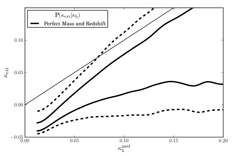
Figure 2 shows the conditional distribution of given , derived from randomly selected Millennium Simulation lines of sight and assuming noise-free halo masses and redshifts. In this case, is almost a delta function since the only uncertainty is halo concentration, which has minimal effect on . At fixed we find in Figure 2 that the scatter in grows with ; our reconstruction is better at reproducing under-dense lines of sight than over-dense lines of sight. The effect of ignoring voids and the smooth mass component is evident in this plot: is significantly higher than , at any given value. Conditioning on gives a PDF for centred at the correct place, by construction.
5.2 How accurate is the calibration?


Let us define the “bias” of the reconstruction of a given line of sight as the difference between the expectation value of over its posterior PDF and the known true value . Let us also define the “width,” , to be half the width of the interval containing the central of the posterior probability .
In an ensemble of reconstructed lines of sight, we find the mean bias to be , and the mean width to be 0.01. This is 1.8 times smaller than the width of the global . We find that our inferred PDFs are consistent with the global distribution; Figure 3 shows that sampling from the inferred from reconstructions of lines of sight produces a distribution of values over the sky nearly identical to the global . Given perfect knowledge of halo mass and redshift then, the calibration procedure provides an unbiased estimate of that is times more precise than using the global . This is the maximum precision we can obtain using the current calibrated halo model.
5.3 Which halos dominate the distribution?
Before investigating the impact of imperfect knowledge of halo mass and redshift, we investigate the uncertainties induced by limits on the magnitude of the observed galaxy sample, and on the field of view. The halos in our catalogue are populated by galaxies and given magnitudes according to the semi-analytic model of De Lucia & Blaizot (2007): by applying magnitude cuts to our catalogue, we can investigate the amount of scatter caused by unobserved halos.
Figure 4 shows the cumulative contribution to as a function of projected distance from the line of sight, magnitude and redshift. We find that most of the convergence comes from halos close to the line of sight. Over half of the convergence typically comes from halos within 30 arcseconds of the line of sight; by 2 arcminutes, this fraction is 85%. The contribution from halos beyond 2 arcminutes is relatively constant at a contribution of 0.0080.003. We find that ignoring halos beyond 2 arcminutes has no effect on the precision of the reconstruction; this is shown in Figure 5. As a function of magnitude, we find that is dominated by objects with magnitudes between and . Objects brighter than are either too rare, or too close to the observer, to make a significant contribution to the convergence. Objects fainter than are too small to be important, unless they are extremely close to the line of sight; we find that including halos fainter than does not improve the reconstruction. Figure 6 shows the scatter on (where is shifted so that its mean is zero, to emulate the effect of the eventual calibration) as a function of reconstruction magnitude limit. We do not expect a deeper survey to decrease the size of the uncertainty in mapping onto . Halos at all redshifts out to the source redshift (1.4 in this work. The redshift of the source in B1608+656) contribute to the convergence, but the largest contribution comes from halos with .


6 Testing the Halo Model Reconstruction on Mock Galaxy Catalogues
We now move on to consider the halo model reconstruction of line-of-sight mass distributions given noisy astronomical observables. A typical imaging survey can be expected to provide measurements of the positions and magnitudes of galaxies in a field; spectra for some of the objects may either come from a synergistic survey, or from targeted follow-up. In this section we quantify the uncertainties induced by inferring the halo mass and redshift from these observables.
As described in Section 4.1, in this work we attempt to infer halo masses from measurements of stellar mass. We will investigate two main sources of uncertainty: the stellar masses themselves, and placing halos at photometric redshifts. Much work has already focused on using photometric colours to infer stellar mass (Auger et al., 2009, e.g. ) and redshifts (Benítez, 2000, e.g. ): we will estimate the likely uncertainties on stellar mass and redshift based on this work.
6.1 Making Mock Observational Catalogues
While the Millennium Simulation catalogues do already contain stellar masses for each galaxy, we do not use them for two reasons. The first is that at the low mass end, the dark matter-only Millennium Simulation satellite galaxy halos are highly stripped relative to what we might expect in a universe containing baryons, leading to a mismatch between the observed and simulated stellar mass–halo mass relations. The second is that we wanted to be able to perform the functional test of trying to recover the convergence having assumed the correct stellar mass–halo mass relation. For these reasons, we assign a new true stellar mass to each halo in the Millennium Simulation catalogues, according to the empirical stellar mass–halo mass relation of Behroozi, Conroy, & Wechsler (2010). When assigning stellar masses we have treated satellites in the same way as central halos; in the real universe both the density profile and the stellar mass–halo mass relation are likely different for satellites and centrals, but our simple model does not include these effects. From these we simulate observed stellar masses by drawing samples from which we take to be a Gaussian of width centred on . Where a spectroscopic redshift exists, stellar masses can be estimated with typical uncertainties of 0.15 dex (Auger et al., 2009); however with photometric redshifts stellar mass uncertainties are typically three times as large. We use dex for halos with a spectroscopic redshift and dex otherwise. For photometric redshift uncertainties we draw a redshift from which we take to be a Gaussian of width centred on , where is the halo’s true redshift in the Millennium Simulation catalogue. In our mock catalogues we have used the galaxy position from the Millennium Simulation; this is not necessarily coincident with the centre of the galaxy’s host dark matter halo.
Given an uncertain stellar mass and redshift it is possible to infer a halo mass using the stellar mass–halo mass relation of Behroozi, Conroy, & Wechsler (2010). This procedure requires an inversion of the relation given in Behroozi, Conroy, & Wechsler (2010) and correctly inverting the relation’s uncertainties requires care: the procedure we use to do this is given in Appendix A. By drawing sample halo masses and redshifts, we can infer a sample using the procedure of Section 4. Repeatedly drawing samples allows us to estimate for each reconstructed line of sight. We then transform this into our target PDF as described above.
6.2 Reconstructing given a spectroscopic redshift for every object


The best possible reconstructions of will come from having a spectroscopic redshift for every single object in each field. Figure 7 shows the distribution of posterior PDF widths for various data qualities: complete spectroscopic coverage results in the smallest widths. In terms of telescope time, such a reconstruction would likely be prohibitively expensive, but we investigate this scenario as an ideal case.
Reconstructing the lines of sight with perfect knowledge of the redshift but an uncertain stellar mass, we find that the width of grows with the expectation of and the ray-traced (Figure 8). The low lines of sight are relatively empty, and so there are few opportunities for uncertainties in the halo masses to propagate into uncertainties; low lines of sight can be reconstructed more precisely than high lines of sight.
6.3 Reconstructing from photometry alone
Inferring the stellar mass of a galaxy from its magnitude and colours requires an estimate of how far away the galaxy is; without a spectroscopic redshift the inferred stellar mass is less precise. However, obtaining photometry has much lower observational cost; all upcoming large area photometric surveys will reach 24th magnitude, providing sufficient data to reconstruct lines of sight without additional observations. In principle the photometric redshift is correlated with the inferred stellar mass, however we do not model this effect since the convergence from the outskirts of an individual halo is only weakly dependent on redshift at fixed mass due to the breadth of the lensing kernel: the redshift uncertainty has only a small effect on the inferred in comparison to that of the uncertain stellar masses. With only photometric redshifts, the uncertainty on is larger than in the spectroscopic case, and this propagates into a broader , as can be seen in Figure 7. However, the photometric reconstruction still typically produces a 50% improvement compared to the precision of the global .
With photometric data alone, can shift by 0.01 relative to given spectroscopic coverage. Since the contribution of voids cannot change with data quality, the shift in must be due to the asymmetric propagation of stellar mass uncertainties into uncertainties. As the stellar mass uncertainty increases, is pushed higher. To correctly calibrate one must include the data quality used to generate .
We find that the width of grows with the expectation value of ; this is shown in Figure 8. The low lines of sight are relatively empty, and so there are few opportunities for uncertainties in the halo masses to propagate into uncertainties.
6.4 Reconstructing with partial spectroscopic coverage
While a fully photometric reconstruction provides useful constraints on , targeted spectroscopy can provide additional constraints on the masses and redshifts of halos whose contributions have the largest absolute uncertainty. Obtaining spectra of bright () objects is relatively fast with large telescopes: however, we find that if spectroscopic redshifts were known for all galaxies in our fields the reconstruction improves only slightly over the purely photometric reconstruction, although the improvement can depend strongly on the details of the particular line of sight. Obtaining spectra for fainter objects would be correspondingly more expensive, but if spectroscopic redshifts could be obtained for all galaxies (as part of a futuristic baryon acoustic oscillation survey, for example) and all galaxies within 1 arcminute of the line of sight, then we find that the would be almost as precise as that from having complete spectroscopic coverage (Figure 7). If any object is extremely close to the lines of sight our approximation of weakly lensing mass-sheets will break down; also, neglecting baryonic effects will also be a poor approximation; a spectrum will be needed to adequately model systems with very well aligned pertrubers. Consistent with our previous findings, the lowest lines of sight have the most constrained PDFs.
7 Systematic Errors due to Sample Selection

While it is good to reconstruct precisely, it is more important that is reconstructed accurately. The reconstruction must not be biased. We quantify the accuracy of our reconstructed in the following way. By shifting the inferred for each line of sight by the true (ray-traced) convergence, we obtain a PDF that should be centred on zero; these offset PDFs can be multiplied together for multiple lines of sight to emulate a joint likelihood analysis, and then test for possible bias in it:
| (9) |
In this section, we quantify the bias as the size of the deviation in the expectation value of from zero. If the bias of is smaller than the half-width of , our inferences can be considered accurate. Since the width of decreases as more sightlines are combined, a small bias will always eventually be found. In the context of measuring time-delay distance at the one percent level, the expectation value of needs to be significantly less than 0.01. External convergence is not the only source of uncertainty in measuring time-delay distance. Since the statistical distance uncertainties due to lens modelling and time delay estimation are likely to be at the 3-4% level (Suyu et al., 2010), convolving with a Gaussian of width is a reasonable approximation for the likely final uncertainty on time-delay distance.
The source of systematic error that we investigate in this paper is that of sample selection: we define three different example selections of lines of sight, and compute the bias that would result (if left unaccounted for) in each one in turn, as a function of data quality. The results described below are illustrated in Figure 9.
7.1 Selecting random lines of sight
We first consider a purely random selection of lines of sight. With the purely photometric reconstruction, there is no evidence of bias, even after combining 20 lines of sight. This result is a sanity check: if we had chosen lines of sight with identical rather than , randomly selected lines of sight would have zero bias by construction. If lines of sight hosting time delay lenses are truly random, our method allows to be reconstructed without inducing a bias (under the basic assumptions that the universe is like the calibration simulation, and the correct stellar-mass to halo-mass relation has been used).
7.2 Selecting only the lines of sight with narrow
Since follow-up campaigns (such as high resolution imaging, or time variability monitoring) are expensive, it is likely that only a subset of detected objects will be observed further. By pre-selecting objects that have the best-constrained convergence, the cosmological value per lens can be increased. However, this selection (like any other) has the potential to induce a bias. It is likely that only photometry will be available at the time of sub-sample selection (although spectroscopic follow-up might be conducted at a later date). We mimic such a selection by drawing lines of sight only from those in the lowest third of , given a purely photometric reconstruction of their fields.
We find that selecting the most tightly constrained lines of sight in this way does not introduce a significant bias: our reconstruction is most accurate for the lowest lines of sight. Combining 20 such systems, the bias is at the 0.001 level.
Photometry of the field seems to be sufficient to adequately select these empty lines of sight. However, since lenses are typically massive galaxies and hence found in locally over-dense environments, it is unlikely that an almost empty line of sight would actually contain a lens; what we can say is that if the local environment can be identified spectroscopically, and then the line of sight mass distribution reconstructed using our method, selecting lenses with low, well-constrained values of will lead to an increase in distance precision at no cost in bias.
7.3 Selecting only high shear lines of sight
Time delay lenses are often selected for follow-up based on their images’ brightness (to make monitoring observations less expensive), their images’ separation (to decrease the covariance between the ground-based image light-curves), or the fact that they are quadruply-imaging rather than doubly-imaging (since this yields 3 time delays instead of 1, a higher magnification and a more informative Einstein Ring system). All three of these properties favour lenses with high convergence and shear along their lines of sight. Focusing on the quad selection, we might expect many of these systems to have significant external shear (since the cross-section for 4 image production is so sensitive to ellipticity in the lens mass distribution (or equivalently, external shear due to the lens’ environment).
We can test the impact of such a shear selection by selecting only lines of sight with an external shear above some threshold. We define a somewhat extreme selection of , and find that in this sample, would be systematically underestimated at the 0.008 level (corresponding to a 0.8% systematic error in distance). In the absence of other sources of uncertainty, this systematic error would be significant in a sample of just 5 lenses; when including other time-delay distance uncertainties a 0.8% bias would be significant for 20 lenses. This systematic error is mitigated if only the lines of sight with both and well constrained are used, but in this case a bias at the 0.005 level remains.
While is likely to be a much stronger selection than would occur in reality, it is nevertheless worth noting from this example that the reconstruction procedure can be biased if lens selection functions are extreme and unaccounted for. Since our model does not include shear constraints it is not surprising that a selection function based on shear can induce a bias. A more sophisticated model that includes the shear recovered from the lens modelling might be less susceptible to this bias.
The halo model can also be used to estimate the external shear along a line of sight: shear is an observable that can be extracted from strong lens modelling. However, there is a degeneracy between internal and external shear. When the Einstein Ring imaging data are very good it is possible to disentangle external and internal shear (Suyu et al., 2010, e.g. ), but there are still significant uncertainties. Wong et al. (2011) attempted to match the shear from strong lens models with a reconstruction of the local lens group environment, but found a tension between the strong lens model and the reconstruction of the environment. Given the Wong et al. (2011) results, it is unclear whether the external shear from lens models can be reconciled with a line-of-sight reconstruction. Alternatively, it may be possible to infer external shear using weak lensing information from near the line of sight. If the true external shear can be measured, it provides an additional constraint on which of the Millennium Simulation lines of sight are similar to the reconstructed line of sight. Suyu et al. (2012) found that in the case of RXJ1131-1231, combining shear constraints with galaxy number count over-density gave a significantly different compared to the PDF from number count over-density alone, .
Extending our model to include shear we find that given perfect knowledge of the halo mass and redshift the ray-traced external shear and the reconstructed external shear are similar, with 68 percent of lines obeying
| (10) |
Future work should investigate whether can be used to improve the accuracy and precision of estimation, given a reconstruction of the line of sight.
8 Systematic Errors due to Assuming an Incorrect Stellar Mass–Halo Mass Relation

Throughout this work we have assumed that the universe’s halos are populated with galaxies whose stellar masses are determined purely by the Behroozi, Conroy, & Wechsler (2010) Stellar Mass–Halo Mass relation, which we then use in our reconstruction. In practice, the true Stellar Mass–Halo Mass relation may well be different to the one we assume in our inference, and if it is, a systematic error could be incurred. It is hard to test the size of this systematic error, since we do not know how much the real universe differs from the chosen Stellar Mass–Halo Mass relation. As wider and deeper surveys are conducted more data will become available with which to construct the Stellar Mass–Halo Mass relation; this should drive the inferred Stellar Mass–Halo Mass relation closer to the truth. We are only interested in testing the effect of changing the Stellar Mass–Halo Mass relation in a way that is consistent with observational constraints; improving the observational constraints on the Stellar Mass–Halo Mass relation will decrease the the potential size of the systematic error on reconstructed induced by assuming a specific Stellar Mass–Halo Mass relation.
To estimate the potential size of this systematic error, we repeat the analysis of the previous section, still using the the Behroozi et al. relation to generate the stellar masses of our calibration lines of sight and hence carry out the inference, but now using simulated catalogue datasets that were generated from the stellar mass–halo mass relation of Moster et al.
This relation provides a comparable fit to the stellar mass function to the Behroozi et al relation, so represents a plausible alternative to our assumed form. For halo masses of , both stellar mass–halo mass relations predict a stellar mass of , but for halos more massive than this the stellar masses generated from the Moster relation are systematically higher than those generated from the Behroozi relation. At halo masses of the predicted stellar masses differ by some dex.
Applying our Behroozi–based reconstruction to lines of sight with Moster stellar masses results in systematic overestimates of . In Figure 10 we show this bias emerging after combining several lines of sight. With a purely photometric reconstruction there is a typical systematic bias of on the reconstructed convergence. This can be shrunk to if only the low lines of sight are used; however for the high shear lines of sight the bias is . It is not too surprising that the low lines of sight are least affected by changes in the stellar mass–halo mass relation. Low lines of sight are relatively empty, their values are small, and they do not depend as strongly on the stellar mass–halo mass relation. In contrast, the high shear lines of sight have significantly overestimated values, since they tend to lie close to massive halos – the regime where the Moster and Behroozi relations are most different. Interestingly, overestimating the values of high shear lines of sight pushes them into the region where the to calibration is least certain; this significantly decreases the precision of the reconstructed .
Despite these systematic errors, we find that the photometric reconstruction is still sufficient to choose the best lines of sight for spectroscopic follow-up. With targeted spectroscopy the systematic error decreases to for the ensemble, for the low kappa sample and for the high shear sample. These results provides further motivation for prioritizing the lenses that reside on the under-dense lines of sight.
The systematic errors reported here are perhaps overly pessimistic, because the bias is due to differences in the stellar masses predicted for high mass halos. If new observations can discriminate between the high mass end of the Behroozi et al. and Moster et al. relations, then the systematic error on the reconstruction will decrease. Similarly, incorporating additional information about the high mass group and cluster-scale halo systems, such as their richness or other occupation statistics, would help mitigate the stellar to halo mass conversion error.
9 Discussion
The total convergence along a line of sight is strongly correlated with the reconstructed . However, since our model ignores voids and assumes all halos follow a spherical truncated-NFW profile our halo model does not include all of the relevant physics; hence, the width of our resulting is still typically 0.01 for any given lightcone, even assuming perfect knowledge of every halo’s virial mass and redshift. To make further progress a more advanced treatment of both voids and halos will be needed. Karpenka et al. (2012) find that their supernova data prefer, in the context of their simple halo model, a truncated isothermal profile for the galaxy mass distributions. Galaxy-galaxy and cluster-galaxy lensing studies (Gavazzi et al., 2007; Johnston et al., 2007; Lagattuta et al., 2010, e.g. ) also suggest an approximately isothermal profile for the mass-shear correlation function; however, at large radii these profiles are dominated by the effects of neighbouring halos, which are already taken into account by our model. Further iterations on the analysis presented here should include the stellar mass distributions that cause the isothermal density profiles in the centres of galaxies, although we do not expect this to have a big impact on the reconstructions. Likewise, halo ellipticity may have some small effect on the predicted convergence. It is possible that baryonic physics may alter the radial profile of dark matter halos, even on large scales. Semboloni et al. (2012) found that baryonic physics had a 30-40% impact on three-point shear statistics, it is unclear how baryons affect one-point convergence statistics compared to the pure dark matter simulations used in this work.
Clusters, filaments and voids are more difficult to model, but simple forms could in principle be derived from the structures found in the simulations, and included in the halo model in some way. Most importantly for the highest lines of sight will be a better group and cluster model: Momcheva et al. (2006) and Wong et al. (2011) recommend using models where dark mass is assigned to both galaxy-scale halos and halos for the groups and clusters they occupy. To make this work, one could incorporate a group and cluster finder, and then infer halo mass from optical richness (Koester et al., 2007, e.g. ) in tandem with BCG stellar mass. A group finder would also allow us to identify central and satellites galaxies; in this work we have neglected the differences between central halos and satellites. However, given perfect knowledge of halo masses we found that only in 5 percent of sightlines do satellites contribute over 20 percent of the sightline’s total . Introducing a group finder is unlikely to provide major improvement to the reconstruction of satellites. Meanwhile, improving the modelling of voids could be done using suggestions by Krause et al. (2012) or Higuchi et al. (2012) combined with a void finder such as in Foster & Nelson (2009). Combining an advanced halo model with a void model will allow a direct test of the halo approximation: using real photometric data one could reconstruct lines of sight and compare against measured weak lensing shears. This would ensure that the reconstruction model reproduces the contents of the real universe, rather than a particular simulation.
The reduction of to just its median value, before using it to look up the appropriate from the simulated sightline ensemble, is reminiscent of the procedure followed by Suyu et al. (2010), and Greene et al. (2013). The reconstruction method presented here can be seen as the limiting case of the weightings explored by Greene et al: rather than using weighted number counts in an aperture, we treat each galaxy individually, and predict for use in their place. Given photometry alone, our reconstruction represents a 50% improvement of the precision compared the number counts used in Suyu et al. (2010). Greene et al. made important progress for the most over-dense lines of sight; our reconstructions are 30% more precise than those of Greene et al. The use of relative over-densities by Suyu et al. and Greene et al. may decrease their sensitivity to the choice of calibration simulation; this work’s use of absolute convergence may be less robust to changes in the calibration simulation.
In this work, we have used the Millennium Simulation as a calibration tool. If the real Universe is not like the Millennium Simulation, then this calibration will be incorrect. Repeating this study using a different simulation to make the test catalogues would allow us to quantify the sensitivity of our results to the simulation used. Similarly the use of a different semi-analytic model to paint galaxies onto halos would enable similar exploration of these systematic errors. Suyu et al. (2010) used the relative over-density to mitigate the effect of simulation and simulation, but it does not completely remove the dependence on simulation. We have tested the effect of using a different stellar mass–halo mass relation and found that this can induce significant systematic biases if the true relation is unknown. Future work should include investigating the robustness of the reconstruction to these systematic errors and develop prescriptions that mitigate against them
10 Conclusions
In this work we have investigated a simple halo model prescription for reconstructing all the mass along a line of sight to an intermediate redshift source. We have used the ray-traced lensing convergence along lines of sight through the Millennium Simulation to calibrate estimates of the total convergence made by summing the convergences due to each object in a photometric catalogue. Having found that the reconstruction process is accurate given this calibration and perfect knowledge of halo mass and redshift, we investigated the effects of reasonable uncertainties in the stellar mass and redshift of each halo, and propagated these uncertainties into a for each line of sight. We also defined three different possible line of sight selections, and investigated the possible bias induced by these selections. We draw the following conclusions:
- •
Despite our model’s simplicity, its reconstructed values are good tracers of . is biased due to our ignorance of voids, groups and clusters, and the unseen mass in small halos and filaments, but we find that this can be calibrated out using the Millennium Simulation catalogues. We found that with perfect knowledge of every halo’s mass and redshift, calibrated reconstruction of a typical line of sight gives an unbiased estimate of that is not perfect, but is times more precise than the global . This factor quantifies the limit to which the halo model can represent the external convergence due to line of sight mass structure.
- •
With uncertain halo masses and redshifts, we find that can still be calibrated in order to infer from the ensemble of simulated lines of sight, but the resulting PDFs tend to be much broader than for perfect halo mass and redshift reconstructions.
- •
It is very rare for halos further than 2 arcminutes from the line of sight to make a significant contribution to ; likewise, including halos whose host galaxy is less luminous than does not significantly improve our reconstructions. A photometric survey to this depth of a 44 arcminute patch around the target would approach the limiting uncertainties of our simple reconstruction recipe, and yield a that has, on average, a width of 0.016 (inducing a 1.6% uncertainty on time-delay distances). This is 1.5 times less broad than the global .
- •
For the most over-dense lines of sight, the reconstruction produces a broad PDF; conversely, we find that the lines of sight with the sharpest inferred are typically under-dense. Since the reconstructions described here can be performed before follow-up time is invested, it will be possible to select targets by the precision of their estimates. This will be useful in an era when there are more known lenses than can be followed-up. Photometric data are sufficient to select the best lines of sight for follow-up. Spectroscopic coverage helps to tighten for most lines of sight.
- •
Selecting from the highest precision 33% of the reconstructed lines of sight results in a sample with low bias, 0.1% in terms of the time-delay distance. For these lines of sight the reconstructed induces a statistical uncertainty of 1% on individual time-delay distances.
- •
Conversely, selecting lines of sight with high shear (; a somewhat extreme selection, but one that could potentially arise from focusing on four-image or wide separation lenses) results in a sample with bias of 0.8% in time delay distance (and hence ). Including realistic estimates of other sources of uncertainty a systematic error of 0.8% would become significant in a sample of 20 lenses. The addition of shear constraints to our model might alleviate this potential systematic.
- •
Reconstructing a line of sight with an incorrect stellar mass–halo mass relation can introduce systematic errors on the inferred time-delay distance at the percent level. This error can be reduced by tightening the observational limits on the stellar mass–halo mass relation at the high mass end.
While we have tested our reconstruction method against realistic simulations of line of sight mass distributions in the Universe, our method is also calibrated to these simulations. Testing this assumption in the short term, and replacing it with an empirical calibration (or hierarchical inference) in the longer term, are worthy goals for future work. The halo model framework is flexible enough to enable many such improvements, including, quite naturally, the incorporation of more information from observations.
Acknowledgements
TEC thanks Vasily Belokurov for supervision, guidance and suggestions. We thank Risa Wechsler and Peter Behroozi for useful discussions and suggestions. We are grateful to the referee for suggesting improvements to the original manuscript. TEC acknowledges support from STFC in the form of a research studentship. PJM was given support by the Kavli Foundation and the Royal Society, in the form of research fellowships. SH and RDB, and CDF, acknowledge support by the National Science Foundation (NSF), grant numbers AST-0807458 and AST-0909119, respectively. SHS, ZG and TT gratefully acknowledge support from the Packard Foundation in the form of a Packard Research Fellowship to TT and from the NSF grant AST-0642621. LVEK acknowledges the support by an NWO-VIDI programme subsidy (programme number 639.042.505). The Millennium Simulation databases used in this paper and the web application providing online access to them were constructed as part of the activities of the German Astrophysical Virtual Observatory.
Our code for reconstructing lines of sight is publicly available at https://github.com/drphilmarshall/Pangloss.
Appendix A Inferring given a noisy measurement of
To estimate the convergence caused by a halo we need to know its mass; how can halo mass be inferred from a noisy estimate of the stellar mass of a galaxy at redshift . We seek the posterior PDF , which can be expanded as follows:
| (11) | |||||
where we have used Bayes’ Theorem twice to replace with , and to invert into the sampling distribution , which we recognise as the likelihood function for the observed stellar mass. Note that the “true” of the galaxy is marginalised out: we are only interested in inferring the halo mass. The last two terms in (11) are the relation from Behroozi, Conroy, & Wechsler (2010), and the halo mass function , at the given redshift. We can tabulate the product of these two from our Millennium Simulation catalogue, constructing a two-dimensional histogram of halo masses and their associated true stellar masses (drawn from the Behroozi relation).
For each galaxy, we compute the likelihood function for its as a function of the unknown , and multiply it by our tabulated joint PDF. This heavily downweights halos with values outside the observed range. We then do the marginalisation integral by Monte Carlo, drawing (two-dimensional) sample parameter vectors from the down weighted histogram, discarding the values, and constructing a one-dimensional histogram that is an estimate of .
If the redshift of the galaxy is uncertain, we need to take this uncertainty into account; for example, for each sample drawn from the photometric redshift posterior PDF , we can draw a sample using the above procedure.
References
- Auger et al. (2007) Auger, M. W., Fassnacht, C. D., Abrahamse, A. L., Lubin, L. M., & Squires, G. K. 2007, AJ, 134, 668
- Auger (2008) Auger, M. W. 2008, MNRAS, 383, L40
- Auger et al. (2009) Auger M. W., Treu T., Bolton A. S., Gavazzi R., Koopmans L. V. E., Marshall P. J., Bundy K., Moustakas L. A., 2009, ApJ, 705, 1099
- Auger et al. (2010) Auger M. W., Treu T., Bolton A. S., Gavazzi R., Koopmans L. V. E., Marshall P. J., Moustakas L. A., Burles S., 2010, ApJ, 724, 511
- Baltz, Marshall, & Oguri (2009) Baltz E. A., Marshall P., Oguri M., 2009, JCAP, 1, 15
- Behroozi, Conroy, & Wechsler (2010) Behroozi P. S., Conroy C., Wechsler R. H., 2010, ApJ, 717, 379
- Benítez (2000) Benítez N., 2000, ApJ, 536, 571
- Bradač et al. (2009) Bradač, M., et al. 2009, ApJ, 706, 1201
- Cropper et al. (2012) Cropper, M., Cole, R., James, A., et al. 2012, arXiv:1208.3369
- Collett et al. (2012) Collett T. E., Auger M. W., Belokurov V., Marshall P. J., Hall A. C., 2012, MNRAS, 424, 2864
- Dalal et al. (2005) Dalal, N., Hennawi, J. F., & Bode, P. 2005, ApJ, 622, 99
- De Lucia & Blaizot (2007) De Lucia G., Blaizot J., 2007, MNRAS, 375, 2
- Fadely et al. (2010) Fadely, R., Keeton, C. R., Nakajima, R., & Bernstein, G. M. 2010, ApJ, 711, 246
- Falco, Gorenstein, & Shapiro (1985) Falco E. E., Gorenstein M. V., Shapiro I. I., 1985, ApJ, 289, L1
- Fassnacht & Lubin (2002) Fassnacht, C. D., & Lubin, L. M. 2002, AJ, 123, 627
- Fassnacht et al. (2006) Fassnacht, C. D., Gal, R. R., Lubin, L. M., et al. 2006, ApJ, 642, 30
- Fassnacht, Koopmans, & Wong (2011) Fassnacht C. D., Koopmans L. V. E., Wong K. C., 2011, MNRAS, 410, 2167
- Foster & Nelson (2009) Foster, C., & Nelson, L. A. 2009, ApJ, 699, 1252
- Gavazzi et al. (2007) Gavazzi, R., Treu, T., Rhodes, J. D., et al. 2007, ApJ, 667, 176
- Gavazzi et al. (2008) Gavazzi R., Treu T., Koopmans L. V. E., Bolton A. S., Moustakas L. A., Burles S., Marshall P. J., 2008, ApJ, 677, 1046
- Greene et al. (2013) Greene, Z. S., Suyu, S. H., Treu, T., et al. 2013, arXiv:1303.3588
- Gunnarsson et al. (2006) Gunnarsson, C., Dahlén, T., Goobar, A., Jönsson, J., Mörtsell, E. 2006, ApJ, 640, 417
- Higuchi et al. (2012) Higuchi, Y., Oguri, M., & Hamana, T. 2012, arXiv:1211.5966
- Hilbert et al. (2007) Hilbert, S., White, S. D. M., Hartlap, J., & Schneider, P. 2007, MNRAS, 382, 121
- Hilbert et al. (2009) Hilbert S., Hartlap J., White S. D. M., Schneider P., 2009, A&A, 499, 31
- Hilbert et al. (2011) Hilbert, S., Gair, J. R., & King, L. J. 2011, MNRAS, 412, 1023
- Holder & Schechter (2003) Holder, G. P., & Schechter, P. L. 2003, ApJ, 589, 688
- Holz & Wald (1998) Holz D. E., Wald R. M., 1998, PhRvD, 58, 063501
- Holz & Linder (2005) Holz, D. E., & Linder, E. V. 2005, ApJ, 631, 678
- Jönsson et al. (2010) Jönsson, J., Dahlén, T., Hook, I., Goobar, A., Mörtsell, E. 2010, MNRAS, 402, 526
- Johnston et al. (2007) Johnston, D. E., Sheldon, E. S., Wechsler, R. H., et al. 2007, arXiv:0709.1159
- Karpenka et al. (2012) Karpenka, N. V., March, M. C., Feroz, F., & Hobson, M. P. 2012, arXiv:1207.3708
- Kauffmann et al. (1999) Kauffmann, G., Colberg, J. M., Diaferio, A., & White, S. D. M. 1999, MNRAS, 303, 188
- Krause et al. (2012) Krause, E., Chang, T.-C., Doré, O., & Umetsu, K. 2012, arXiv:1210.2446
- Keeton & Zabludoff (2004) Keeton, C. R., & Zabludoff, A. I. 2004, ApJ, 612, 660
- Keeton & Moustakas (2009) Keeton C. R., Moustakas L. A., 2009, ApJ, 699, 1720
- Koester et al. (2007) Koester, B. P., McKay, T. A., Annis, J., et al. 2007, ApJ, 660, 221
- Koopmans et al. (2003) Koopmans, L. V. E., Treu, T., Fassnacht, C. D., Blandford, R. D., & Surpi, G. 2003, ApJ, 599, 70
- Koopmans (2004) Koopmans, L. V. E. 2004, arXiv:astro-ph/0412596
- Lagattuta et al. (2010) Lagattuta, D. J., Fassnacht, C. D., Auger, M. W., et al. 2010, ApJ, 716, 1579
- LSST Science Collaboration (2009) LSST Science Collaboration: Abell, P. A., Allison, J., et al. 2009, arXiv:0912.0201
- Macciò et al. (2008) Macciò, A. V., Dutton, A. A., & van den Bosch, F. C. 2008, MNRAS, 391, 1940
- Mandelbaum et al. (2009) Mandelbaum, R., van de Ven, G., & Keeton, C. R. 2009, MNRAS, 398, 635
- Momcheva et al. (2006) Momcheva, I., Williams, K., Keeton, C., & Zabludoff, A. 2006, ApJ, 641, 169
- Moster et al. (2010) Moster, B. P., Somerville, R. S., Maulbetsch, C., et al. 2010, ApJ, 710, 903
- Nakajima et al. (2009) Nakajima, R., Bernstein, G. M., Fadely, R., Keeton, C. R., & Schrabback, T. 2009, ApJ, 697, 1793
- Navarro, Frenk, & White (1997) Navarro J. F., Frenk C. S., White S. D. M., 1997, ApJ, 490, 493
- Neto et al. (2007) Neto A. F., et al., 2007, MNRAS, 381, 1450
- Oguri & Takahashi (2006) Oguri, M., & Takahashi, K. 2006, Phys. Rev. D, 73, 123002
- Oguri & Marshall (2010) Oguri M., Marshall P. J., 2010, MNRAS, 405, 2579
- Oke (1974) Oke J. B., 1974, ApJS, 27, 21
- Schneider (2006) Schneider, P. 2006, in Saas-Fee Advanced Course 33: Gravitational Lensing: Strong, Weak and Micro, 269
- Semboloni et al. (2012) Semboloni, E., Hoekstra, H., & Schaye, J. 2012, arXiv:1210.7303
- Springel et al. (2005) Springel V., et al., 2005, Natur, 435, 629
- Suyu (2012) Suyu, S. H. 2012, MNRAS, 426, 868
- Suyu et al. (2012) Suyu S. H., et al., 2012, arXiv, arXiv:1208.6010
- Suyu et al. (2010) Suyu S. H., Marshall P. J., Auger M. W., Hilbert S., Blandford R. D., Koopmans L. V. E., Fassnacht C. D., Treu T., 2010, ApJ, 711, 201
- Takahashi et al. (2011) Takahashi, R., Oguri, M., Sato, M., & Hamana, T. 2011, ApJ, 742, 15
- Treu et al. (2009) Treu, T., Gavazzi, R., Gorecki, A., et al. 2009, ApJ, 690, 670
- Vale & White (2003) Vale C., White M., 2003, ApJ, 592, 699
- Wambsganss et al. (2004) Wambsganss, J., Bode, P., & Ostriker, J. P. 2004, ApJL, 606, L93
- Wang & Dai (2011) Wang, F. Y., & Dai, Z. G. 2011, A&A, 536, A96
- Williams et al. (2006) Williams, K. A., Momcheva, I., Keeton, C. R., Zabludoff, A. I., & Lehár, J. 2006, ApJ, 646, 85
- Wong et al. (2011) Wong K. C., Keeton C. R., Williams K. A., Momcheva I. G., Zabludoff A. I., 2011, ApJ, 726, 84
- Wong et al. (2012) Wong, K. C., Ammons, S. M., Keeton, C. R., & Zabludoff, A. I. 2012, ApJ, 752, 104
- Wyithe et al. (2011) Wyithe, J. S. B., Yan, H., Windhorst, R. A., & Mao, S. 2011, Nature, 469, 181