Lepton number and flavour violation in TeV-scale left-right symmetric theories with large left-right mixing

James Barry Note: E-mail: james.barry@mpi-hd.mpg.de Affiliation: Max-Planck-Institut für Kernphysik,
Saupfercheckweg 1, 69117 Heidelberg, Germany Werner Rodejohann Note: E-mail: werner.rodejohann@mpi-hd.mpg.de Affiliation: Max-Planck-Institut für Kernphysik,
Saupfercheckweg 1, 69117 Heidelberg, Germany

Abstract

The various diagrams leading to neutrinoless double beta decay in the left-right symmetric model have different relative magnitudes, depending on the scale of new physics. Neutrinos acquire mass from both type I and/or type II seesaw terms, making an unambiguous analysis difficult. We study the half-life for double beta decay in the case of type II and type I dominance, in the former case including interference terms. If the heavy neutrinos of the type I seesaw model are at the TeV scale, certain processes can be enhanced. In particular, there are regions of parameter space in which the so-called $\lambda$ - and $\eta$ -diagrams can give sizable contributions to the half-life for the decay. We perform a detailed study of one such scenario, paying careful attention to constraints from lepton flavour violation.

1 Introduction

Neutrinoless double beta decay ( $0\nu\beta\beta$ ) is a lepton number violating process, which, if observed, would prove that neutrinos are Majorana particles [1]. New physics beyond the standard model is required to make the process observable [2], and there are several different theoretical frameworks that could provide the necessary operators (see the review in Ref. [3]). One of those theories is the left-right symmetric model (LRSM) [4, 5, 6, 7, 8], in which parity is restored at high energies and right-handed neutrinos are naturally included as part of an $SU(2)$ doublet of the extended gauge symmetry. In that case there are a number of new physics contributions to $0\nu\beta\beta$ , either from right-handed neutrinos or Higgs triplets, with the rate for double beta decay linked to neutrino mass. This connection can be both indirect, through the couplings to and/or mixing with right-handed neutrinos, as well as direct, via the standard light neutrino contribution (see Refs. [9, 7, 10] for some of the first discussions of $0\nu\beta\beta$ in the LRSM).

In the simplest version of the LRSM one expects the scale of parity restoration to be rather high, i.e., around the GUT scale of $10^{15}$ GeV. Indeed, if all couplings in the scalar potential of the theory are of order one then this conclusion follows naturally [8]. Nevertheless, there is still enough freedom in parameter space to allow one to consider TeV-scale left-right symmetry, which leads to several distinct and observable signatures in present-day experiments probing leptonic processes. On the other hand, the quark sector of the TeV-scale model is severely constrained, due to the presence of flavour changing neutral currents (FCNCs) induced by the neutral components of Higgs bidoublets that are introduced to break electroweak symmetry. These affect meson mixing, $CP$ violation in meson decay and the neutron electric dipole moment, and one needs the neutral component of the Higgs bidoublet to be heavier than about $15$ TeV [11] to avoid conflict with experiment. The mass of the right-handed $W$ -boson ( $W_{R}$ ) can however still be around $3$ TeV, and current LHC data is already beginning to probe $W_{R}$ masses of this order [12, 13]. Indeed, the latest limits from the CMS experiment are roughly $m_{W_{R}}\mathrel{\hbox to0.0pt{\raise 2.20013pt\hbox{$>$}\hss}{\lower 2.20013pt\hbox{$\sim$}}}2.5$ TeV (see Fig. 6). With right-handed neutrinos of similar mass or lighter there are observable effects in $0\nu\beta\beta$ and lepton flavour violation (LFV). The connection between double beta decay, LHC and lepton flavour violation has recently been studied by several authors [14, 15, 16, 17, 18, 19, 20].

From the theoretical point of view, the LRSM provides a natural framework for both the type I [21, 22, 23, 9, 24] and type II [25, 26, 27, 7, 28, 29] seesaw mechanisms, mediated by right-handed neutrinos and Higgs triplets, respectively. In this way the smallness of neutrino mass is connected to the restoration of parity at high energies, and the $0\nu\beta\beta$ process can proceed via the same mediators that lead to neutrino mass. It is however rather difficult to pin down the mechanism by which the process occurs. A simplified case that has already been studied in the literature is that of type II seesaw dominance for $m_{\nu}$ [14], which restricts the number of parameters by making the right- and left-handed Majorana mass terms proportional to each other. We perform a detailed investigation of this case including LFV constraints explicitly in the calculation of the $0\nu\beta\beta$ half-life, and show that there are indeed places in parameter space where the triplet contribution can be significant and can interfere with the other contributions.

The case of type I seesaw dominance is more complicated: there are some contributions to $0\nu\beta\beta$ that involve the left- and right-handed sectors individually as well as others that involve both sectors, through “left-right mixing”. A simplified version was studied in Ref. [17], and a useful formula relating the various mass matrices of the theory was presented in Ref. [18], for the case of symmetric Dirac coupling. Since the left-right mixing is always a ratio of the Dirac and Majorana mass scales, $0\nu\beta\beta$ processes involving left-right mixing can be enhanced for specific Dirac mass matrices. This enhancement [30, 31] is also required for collider signatures of the TeV-scale type I seesaw mechanism with left-handed currents (see the review in Ref. [32]), and there have been several studies of related phenomenology [33, 34, 35, 36]¹¹ 1 In the LRSM one can produce right-handed neutrinos at the LHC via right-handed currents [37], as will be discussed in Section 3.3.. In the LRSM case both the so-called $\lambda$ - and $\eta$ -diagrams could give large contributions, although the latter is further suppressed by the mixing between left- and right-handed gauge bosons. This idea has also been discussed in the context of the inverse process $e^{-}e^{-}\rightarrow W_{L}^{-}W_{R}^{-}$ [38], was further emphasized in extended seesaw versions of the LRSM [19, 20] and a recent analysis of mixed diagrams at the LHC can be found in Ref. [39]. We perform a thorough analysis of the type I seesaw scenario, paying attention to the correct nuclear matrix elements for the different diagrams as well as the often severe constraints from lepton flavour violating phenomena.

The paper is outlined as follows: in Section 2 we briefly summarize the theoretical details of the left-right symmetric model (the reader familiar with the LRSM may skip this section), and in Section 3 we provide a detailed discussion of the $0\nu\beta\beta$ and LFV processes in the model. Section 4 is a quantitative analysis of the various $0\nu\beta\beta$ amplitudes in the limit of type I or type II seesaw dominance; we summarize and conclude in Section 5. A brief comment on the correlation between $0\nu\beta\beta$ half-lives is given in Appendix A. Details of decay widths and loop functions for LFV processes can be found in Appendix B, which the reader may skip as well; an explicit numerical example demonstrating large left-right mixing is given in Appendix C.

2 The left-right symmetric model

In the left-right symmetric model, the Standard Model is extended to include the gauge group $SU(2)_{R}$ (with gauge coupling $g_{R}\neq g_{L}$ ), and right-handed fermions are grouped into doublets under this group. Thus we have the following fermion particle content under $SU(2)_{L}\times SU(2)_{R}\times U(1)_{B-L}$ :

	$\displaystyle L^{\prime}_{Li}$	$\displaystyle=\begin{pmatrix}\nu^{\prime}_{L}\\ \ell^{\prime}_{L}\end{pmatrix}_{i}\,\sim(\mathbf{2},\mathbf{1},\mathbf{-1})\,,$	$\displaystyle L^{\prime}_{Ri}=\begin{pmatrix}\nu^{\prime}_{R}\\ \ell^{\prime}_{R}\end{pmatrix}_{i}\sim(\mathbf{1},\mathbf{2},\mathbf{-1})\,,$		(1)
	$\displaystyle Q^{\prime}_{Li}$	$\displaystyle=\begin{pmatrix}u^{\prime}_{R}\\ d^{\prime}_{R}\end{pmatrix}_{i}\,\sim(\mathbf{2},\mathbf{1},\mathbf{\frac{1}{3}})\,,$	$\displaystyle Q^{\prime}_{Ri}=\begin{pmatrix}u^{\prime}_{R}\\ d^{\prime}_{R}\end{pmatrix}_{i}\sim(\mathbf{1},\mathbf{2},\mathbf{\tfrac{1}{3}})\,,$		(2)

with the electric charge given by $Q=T_{L}^{3}+T_{R}^{3}+\frac{B-L}{2}$ and $i=1,2,3$ . The subscripts $L$ and $R$ are associated with the projection $P_{L,R}=\frac{1}{2}(1\mp\gamma_{5})$ . In order to break the gauge symmetry and allow Majorana mass terms for neutrinos one introduces the Higgs triplets

\Delta_{L,R}\equiv\begin{pmatrix}\delta_{L,R}^{+}/\sqrt{2}&\delta_{L,R}^{++}\\ \delta_{L,R}^{0}&-\delta_{L,R}^{+}/\sqrt{2}\end{pmatrix},

(3)

with $\Delta_{L}\sim(\mathbf{3},\mathbf{1},\mathbf{2})$ and $\Delta_{R}\sim(\mathbf{1},\mathbf{3},\mathbf{2})$ ; the electroweak symmetry is broken by the bi-doublet scalar

\phi\equiv\begin{pmatrix}\phi_{1}^{0}&\phi_{2}^{+}\\ \phi_{1}^{-}&\phi_{2}^{0}\end{pmatrix}\sim(\mathbf{2},\mathbf{2},\mathbf{0})\,.

(4)

The relevant Lagrangian in the lepton sector is

\displaystyle{\cal L}^{\ell}_{Y}=

\displaystyle-\overline{L}^{\prime}_{L}(f\phi+\tilde{f}\tilde{\phi})L^{\prime}_{R}-\overline{L}^{\prime c}_{L}i\sigma_{2}\Delta_{L}h_{L}L^{\prime}_{L}-\overline{L}^{\prime c}_{R}i\sigma_{2}\Delta_{R}h_{R}L^{\prime}_{R}+{\rm h.c.},

(5)

where $\tilde{\phi}\equiv\sigma_{2}\phi^{*}\sigma_{2}$ ; $f,g$ and $h_{L,R}$ are matrices of Yukawa couplings and charge conjugation is defined as

(\psi_{L,R})^{c}\equiv{\cal C}\overline{\psi}_{L,R}^{T}=(\psi^{c})_{R,L}\,,\quad{\cal C}\equiv i\gamma_{2}\gamma_{0}\,.

(6)

If one assumes a discrete LR symmetry in addition to the additional gauge symmetry, the gauge couplings become equal ( $g_{L}=g_{R}=g$ ) and one obtains relations between the Yukawa coupling matrices in the model. With a discrete parity symmetry ( $L_{L}\leftrightarrow L_{R}$ , $\phi\leftrightarrow\phi^{\dagger}$ , $\Delta_{L}\leftrightarrow\Delta^{*}_{R}$ ) it follows that $h_{L}=h_{R}^{*}$ , $f=f^{\dagger}$ , $\tilde{f}=\tilde{f}^{\dagger}$ ; with a charge conjugation symmetry ( $L_{L}\leftrightarrow(L_{R})^{c}$ , $\phi\leftrightarrow\phi^{T}$ , $\Delta_{L}\leftrightarrow\Delta_{R}$ ) we have $h\equiv h_{L}=h_{R}$ , $f=f^{T}$ , $\tilde{f}=\tilde{f}^{T}$ . Applying these symmetries simplifies various expressions in the model, as will be discussed later.

Making use of the gauge symmetry to eliminate complex phases, the most general vacuum is

\displaystyle\langle\phi\rangle=\begin{pmatrix}\kappa_{1}/\sqrt{2}&0\\ 0&\kappa_{2}e^{i\alpha}/\sqrt{2}\end{pmatrix},\quad\langle\Delta_{L}\rangle=\begin{pmatrix}0&0\\ v_{L}e^{i\theta_{L}}/\sqrt{2}&0\end{pmatrix},\quad\langle\Delta_{R}\rangle=\begin{pmatrix}0&0\\ v_{R}/\sqrt{2}&0\end{pmatrix}.

(7)

After spontaneous symmetry breaking, the mass term for the charged leptons is

{\cal L}^{\ell}_{\rm mass}=-\overline{\ell}^{\prime}_{L}M_{\ell}\ell^{\prime}_{R}+{\rm h.c.},

(8)

where the mass matrix

M_{\ell}=\frac{1}{\sqrt{2}}(\kappa_{2}e^{i\alpha}f+\kappa_{1}\tilde{f})

(9)

can be diagonalized by the bi-unitary transformation

\ell^{\prime}_{L,R}\equiv V_{L,R}^{\ell}\ell_{L,R}\,,\quad V_{L}^{\ell\dagger}M_{\ell}V_{R}^{\ell}={\rm diag}(m_{e},m_{\mu},m_{\tau})\,.

(10)

With a discrete parity (charge conjugation) symmetry, $M_{\ell}$ becomes hermitian (symmetric), so that the condition $V_{L}^{\ell}=V_{R}^{\ell}$ ( $V_{L}^{\ell}={V_{R}^{\ell}}^{*}$ ) holds. In the neutrino sector we have a type I + II seesaw scenario,

\displaystyle{\cal L}^{\nu}_{\rm mass}=-\tfrac{1}{2}\overline{n^{\prime}_{L}}M_{\nu}n^{\prime c}_{L}+{\rm h.c.}=-\tfrac{1}{2}\begin{pmatrix}\overline{\nu^{\prime}_{L}}\ \overline{{\nu^{\prime}_{R}}^{c}}\end{pmatrix}\begin{pmatrix}M_{L}&M_{D}\\ M_{D}^{T}&M_{R}\end{pmatrix}\begin{pmatrix}{\nu^{\prime}_{L}}^{c}\\ \nu^{\prime}_{R}\end{pmatrix}+{\rm h.c.},

(11)

with

\displaystyle M_{D}=\frac{1}{\sqrt{2}}(\kappa_{1}f+\kappa_{2}e^{-i\alpha}\tilde{f})\,,\quad M_{L}=\sqrt{2}v_{L}e^{i\theta_{L}}h_{L}\,,\quad M_{R}=\sqrt{2}v_{R}h_{R}\,.

(12)

Again, with a parity (charge conjugation) symmetry we have $M_{D}=M_{D}^{\dagger}$ ( $M_{D}=M^{T}_{D}$ ). In the most general case the phase $\theta_{L}$ cannot be set to zero, but in the type II dominance case we will study it is simply an overall phase and has no effect on the resulting neutrino mass matrix (in the type I dominance case it plays no role since $v_{L}=0$ ). Due to the presence of the so-called “VEV seesaw” relation relating the various VEVs, one expects $x\equiv v_{L}v_{R}/\kappa^{2}_{+}={\cal O}(1)$ , since $x$ is a function of (order one) couplings in the scalar potential [8]. However, from a purely phenomenological point of view, $x$ can take any value between 0 and $10^{14}$ [40]. Assuming that $M_{L}\ll M_{D}\ll M_{R}$ , the light neutrino mass matrix can be written in terms of the model parameters as

\displaystyle m_{\nu}=M_{L}-M_{D}M_{R}^{-1}M_{D}^{T}=\sqrt{2}v_{L}e^{i\theta_{L}}h_{L}-\frac{\kappa_{+}^{2}}{\sqrt{2}v_{R}}h_{D}h_{R}^{-1}h_{D}^{T}\,,

(13)

where

h_{D}\equiv\frac{1}{\sqrt{2}}\frac{\kappa_{1}f+\kappa_{2}e^{-i\alpha}\tilde{f}}{\kappa_{+}}\,,\quad\kappa_{+}^{2}\equiv|\kappa_{1}|^{2}+|\kappa_{2}|^{2}\,.

(14)

The symmetric $6\times 6$ neutrino mass matrix $M_{\nu}$ in Eq. (11) is diagonalized by the unitary $6\times 6$ matrix [41, 42, 43]

W\equiv\begin{pmatrix}V_{L}^{\nu}\\ V_{R}^{\nu}\end{pmatrix}=\begin{pmatrix}U&S\\ T&V\end{pmatrix}\simeq\begin{pmatrix}\mathbb{1}-\frac{1}{2}RR^{\dagger}&R\\ -R^{\dagger}&\mathbb{1}-\frac{1}{2}R^{\dagger}R\end{pmatrix}\begin{pmatrix}V_{\nu}&0\\ 0&V_{R}\end{pmatrix}\,

(15)

to $W^{\dagger}M_{\nu}W^{*}={\rm diag}(m_{1},m_{2},m_{3},M_{1},M_{2},M_{3})$ , where the unitary matrices $V_{\nu}$ and $V_{R}$ are defined by

\begin{array}[]{c}M_{L}-M_{D}M_{R}^{-1}M_{D}^{T}=V_{\nu}\,{\rm diag}(m_{1},m_{2},m_{3})\,V_{\nu}^{T},\\[2.84526pt] M_{R}=V_{R}\,{\rm diag}(M_{1},M_{2},M_{3})V_{R}^{T}\,,\end{array}

(16)

and the matrix $R=M_{D}M_{R}^{-1}+{\cal O}(M_{D}^{3}(M_{R}^{-1})^{3})$ describes the left-right mixing. The neutrino mass eigenstates $n=n_{L}+n^{c}_{L}=n^{c}$ are defined by

\displaystyle\begin{split}n^{\prime}_{L}&=\begin{pmatrix}\nu^{\prime}_{L}\\ {\nu^{\prime}_{R}}^{c}\end{pmatrix}=Wn_{L}=\begin{pmatrix}U&S\\ T&V\end{pmatrix}\begin{pmatrix}\nu_{L}\\ N^{c}_{R}\end{pmatrix},\\[2.84526pt] n^{\prime c}_{L}&=\begin{pmatrix}{\nu^{\prime}_{L}}^{c}\\ \nu^{\prime}_{R}\end{pmatrix}=W^{*}n^{c}_{L}=\begin{pmatrix}U^{*}&S^{*}\\ T^{*}&V^{*}\end{pmatrix}\begin{pmatrix}\nu^{c}_{L}\\ N_{R}\end{pmatrix}.\end{split}

(17)

Note that the unitarity of $W$ leads to the useful relations

V_{L}^{\nu}V_{L}^{\nu\dagger}=UU^{\dagger}+SS^{\dagger}=\mathbb{1}=V_{R}^{\nu}V_{R}^{\nu\dagger}=TT^{\dagger}+VV^{\dagger}\,\quad{\rm and}\quad V_{L}^{\nu}V_{R}^{\nu\dagger}=UT^{\dagger}+SV^{\dagger}=0\,,

(18)

with the unitary $3\times 6$ matrices $V^{\nu}_{L}=(U\ \ S)$ and $V^{\nu}_{R}=(T\ \ V)$ defined in Eq. (15).

The leptonic charged current interaction in the flavour basis is

{\cal L}^{\rm lep}_{CC}=\frac{g}{\sqrt{2}}\left[\overline{\ell^{\prime}}\gamma^{\mu}P_{L}\nu^{\prime}W_{L\mu}^{-}+\overline{\ell^{\prime}}\gamma^{\mu}P_{R}\nu^{\prime}W_{R\mu}^{-}\right]+{\rm h.c.},

(19)

where

\begin{pmatrix}W_{L}^{\pm}\\ W_{R}^{\pm}\end{pmatrix}=\begin{pmatrix}\cos\xi&\sin\xi\,e^{i\alpha}\\ -\sin\xi\,e^{-i\alpha}&\cos\xi\end{pmatrix}\begin{pmatrix}W_{1}^{\pm}\\ W_{2}^{\pm}\end{pmatrix}

(20)

characterizes the mixing between left- and right-handed gauge bosons, with $\tan 2\xi=-\frac{2\kappa_{1}\kappa_{2}}{v_{R}^{2}-v_{L}^{2}}$ . With negligible mixing the gauge boson masses become

m_{W_{L}}\simeq m_{W_{1}}\simeq\frac{g}{2}\kappa_{+}\,,\quad{\rm and}\quad m_{W_{R}}\simeq m_{W_{2}}\simeq\frac{g}{\sqrt{2}}v_{R}\,,

(21)

and assuming that²² 2 This is justified if one assumes no cancellations in generating quark masses [44]. $\kappa_{2}<\kappa_{1}$ , it follows that

\xi\simeq-\kappa_{1}\kappa_{2}/v_{R}^{2}\simeq-2\frac{\kappa_{2}}{\kappa_{1}}\left(\frac{m_{W_{L}}}{m_{W_{R}}}\right)^{2},

(22)

so that the mixing angle $\xi$ is at most³³ 3 Although the experimental limit is $\xi<10^{-2}$ [45], for $m_{W_{R}}={\cal O}({\rm TeV})$ one has $\xi\mathrel{\hbox to0.0pt{\raise 2.20013pt\hbox{$<$}\hss}{\lower 2.20013pt\hbox{$\sim$}}}10^{-3}$ [46]; supernova bounds for right-handed neutrinos lighter than 1 MeV are even more stringent ( $\xi<3\times 10^{-5}$ ) [46, 47]. the square of the ratio of left and right scales $(L/R)^{2}$ . Here we assume $L\simeq 10^{2}$ GeV corresponds to the electroweak scale and $R\simeq$ TeV to the scale of parity restoration, $v_{R}$ . For small $\xi$ the charged current in the mass basis becomes

{\cal L}^{\rm lep}_{CC}=\frac{g}{\sqrt{2}}\left[\overline{\ell_{L}}\gamma^{\mu}K_{L}n_{L}(W_{1\mu}^{-}+\xi e^{i\alpha}W_{2\mu}^{-})+\overline{\ell_{R}}\gamma^{\mu}K_{R}n^{c}_{L}(-\xi e^{-i\alpha}W_{1\mu}^{-}+W_{2\mu}^{-})\right]+{\rm h.c.}

(23)

Here $K_{L}$ and $K_{R}$ are $3\times 6$ mixing matrices

K_{L}\equiv V_{L}^{\ell\dagger}V_{L}^{\nu}\,,\quad{\rm and}\quad K_{R}\equiv V_{R}^{\ell\dagger}V_{R}^{\nu*}\,,

(24)

connecting the three charged lepton mass eigenstates $\ell_{i}$ to the six neutrino mass eigenstates $(\nu_{i},N_{i})^{T}$ , ( $i=1,2,3$ ), with [using Eq. (18)] $K_{L}K_{L}^{\dagger}=K_{R}K_{R}^{\dagger}=\mathbb{1}$ and $K_{L}K_{R}^{T}=0$ . The standard neutrino mixing matrix is just the left half of $K_{L}$ , i.e., $U_{\rm PMNS}=V_{L}^{\ell\dagger}U$ .

In this model one also expects a new neutral gauge boson, $Z^{\prime}$ , which mixes with the standard model $Z$ boson. The mass eigenstates $Z_{1,2}$ have the masses

m_{Z_{1}}\simeq\frac{g}{2\cos\theta_{W}}\kappa_{+}\simeq\frac{m_{W_{1}}}{\cos\theta_{W}}\,,\quad{\rm and}\quad m_{Z_{2}}\simeq\frac{g\cos\theta_{W}}{\sqrt{\cos 2\theta_{W}}}v_{R}\simeq\sqrt{\frac{2\cos^{2}\theta_{W}}{\cos 2\theta_{W}}}\,m_{W_{2}}\,,

(25)

where $g=e/\sin\theta_{W}$ and the $U(1)$ coupling constant is $g^{\prime}\equiv e/\sqrt{\cos 2\theta_{W}}$ . Again one expects the mixing to be of order $(L/R)^{2}$ , i.e.,

\phi=-\frac{1}{2}\sin^{-1}\frac{g^{2}\kappa_{+}^{2}\sqrt{\cos\,2\theta_{W}}}{2c_{W}^{2}(m_{Z_{2}}^{2}-m_{Z_{1}}^{2})}\simeq-\frac{m_{Z_{1}}^{2}\sqrt{\cos\,2\theta_{W}}}{m_{Z_{2}}^{2}-m_{Z_{1}}^{2}}\simeq-\sqrt{\cos\,2\theta_{W}}\left(\frac{m_{Z_{1}}}{m_{Z_{2}}}\right)^{2}.

(26)

Eqs. (21) and (25) imply that $m_{Z_{2}}\simeq 1.7m_{W_{2}}$ . The current limits [45, 48] on the neutral gauge boson parameters are $m_{Z^{\prime}}>1.162$ TeV and $|\phi|<1.2\times 10^{-3}$ . In addition, the current limits on the doubly charged triplet masses are [49] $m_{\delta^{\pm\pm}_{L}}>409$ GeV and $m_{\delta^{\pm\pm}_{R}}>322$ GeV. The theory predicts $m_{\delta^{\pm\pm}_{L,R}}\simeq v_{R}$ , assuming order one coupling constants in the scalar potential.

3 $0\nu\beta\beta$ , lepton flavor violation and collider physics

3.1 Neutrinoless double beta decay

3.1.1 Particle physics amplitudes

Here we summarize the various possible diagrams for $0\nu\beta\beta$ in left-right symmetric models (for one of the first analyses on this topic, see Ref. [10]). The Lagrangian in Eq. (23) can be written as

\displaystyle\begin{split}{\cal L}^{\rm lep}_{CC}&=\frac{g}{\sqrt{2}}\sum_{i=1}^{6}\left[\overline{e}\,\gamma^{\mu}(K_{L})_{ei}P_{L}n_{i}(W_{1\mu}^{-}+\xi e^{i\alpha}W_{2\mu}^{-})\right.\\ &\quad+\left.\overline{e}\,\gamma^{\mu}(K_{R})_{ei}P_{R}n_{i}(-\xi e^{-i\alpha}W_{1\mu}^{-}+W_{2\mu}^{-})\right]+{\rm h.c.}\\ &=\frac{g}{\sqrt{2}}\sum_{i=1}^{3}\left[\overline{e_{L}}\gamma^{\mu}(U_{ei}\nu_{Li}+S_{ei}N^{c}_{Ri})(W_{1\mu}^{-}+\xi e^{i\alpha}W_{2\mu}^{-})\right.\\ &\quad+\left.\overline{e_{R}}\gamma^{\mu}(T^{*}_{ei}\nu^{c}_{Li}+V^{*}_{ei}N_{Ri})(-\xi e^{-i\alpha}W_{1\mu}^{-}+W_{2\mu}^{-})\right]+{\rm h.c.},\end{split}

(27)

where in the second line we have assumed a basis where the charged leptons are diagonal (we will use this basis from now on, thus expressing all processes in terms of the matrices $U$ , $S$ , $T$ and $V$ ). $0\nu\beta\beta$ amplitudes arise from second order terms in perturbation theory: it is clear that one can combine either two left-handed currents, two right-handed currents or one left- and one right-handed current. The relevant mixing matrix element also depends on whether light or heavy neutrinos are exchanged in the process; the matrices $U$ , $V$ , $S$ and $T$ are (to second order in $M_{D}/M_{R}$ )

\displaystyle\begin{split}U&\equiv\left[\mathbb{1}-\frac{1}{2}M_{D}M_{R}^{-1}(M_{D}M_{R}^{-1})^{\dagger}\right]V_{\nu},\quad V\equiv\left[\mathbb{1}-\frac{1}{2}(M_{D}M_{R}^{-1})^{\dagger}M_{D}M_{R}^{-1}\right]V_{R},\\[2.84526pt] S&\equiv M_{D}M_{R}^{-1}V_{R},\quad T\equiv-(M_{D}M_{R}^{-1})^{\dagger}V_{\nu}\,,\end{split}

(28)

as defined in Eq. (15), showing that light neutrino mixing is no longer unitary. The additional possibility of $W_{L}-W_{R}$ mixing allows for diagrams with, for instance, two left-handed hadronic currents but one left- and one right-handed leptonic current [see Fig. 4(b)], with the corresponding suppression factor of $\tan\xi$ [Eq. (22)].

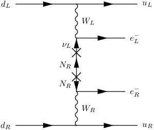
Neutrinoless double beta decay processes in the LR model can be categorized in terms of their topology and the helicity of the final state electrons; the most relevant diagrams that will be discussed in detail in what follows are shown in Figs. 1, 3 and 4 (see Refs. [50] for a complete list). Table 1 contains a summary of the relevant amplitudes as well as limits on the particle physics parameters calculated using the recent KamLAND-Zen limit [51]⁴⁴ 4 The recent GERDA limit [52] on the half-life (see Table 3) does not improve on the limits given here. and the matrix elements in Table 2. Note that the chiral structure of the matrix element means that the neutrino propagator becomes [53]

P_{L,R}\frac{\not{q}+m_{i}}{q^{2}-m_{i}^{2}}P_{L,R}=\frac{m_{i}}{q^{2}-m_{i}^{2}\texttimes}\,\quad{\rm or}\quad P_{L,R}\frac{\not{q}+m_{i}}{q^{2}-m_{i}^{2}}P_{R,L}=\frac{\not{q}}{q^{2}-m_{i}^{2}\texttimes}\,,

(29)

leading to mass or momentum dependence when the leptonic vertices have the same or opposite chirality, respectively, and providing a useful way to categorize the different possible mechanisms. In order to give a very rough estimate of the relative magnitudes we denote the masses of all particles belonging to the right-handed sector ( $M_{i}$ , $W_{R}$ and $\delta_{R}$ ) as $R\simeq$ TeV, and those from the left-handed sector as $L\simeq 10^{2}$ GeV (corresponding to the weak scale, or the mass of the $W_{L}$ ). The matrices $T$ and $S$ describing left-right mixing can be written as $L/R$ , and the gauge boson mixing angle $\xi$ is of order $(L/R)^{2}$ . Note that with this definition the order of magnitude of the type I seesaw contribution is $m_{\nu}\simeq L^{2}/R$ , which is far too large in the naive case (without cancellations), but the estimates made above are still reliable. The typical scale of momentum transfer is $|q|\simeq 100$ MeV.

\minisec

Mass-dependent mechanisms

In this case the emitted electrons have the same chirality and there are either light or heavy neutrinos exchanged, with mass denoted by $m_{i}$ and $M_{i}$ . With both electrons left-handed the amplitude is proportional to

{\cal A}_{LL}\simeq G_{F}^{2}\left(1+2\tan\xi+\tan^{2}\!\xi\right)\sum_{i}\left(\frac{U_{ei}^{2}m_{i}}{q^{2}}-\frac{S_{ei}^{2}}{M_{i}}\right),

(30)

whereas if both are right-handed it becomes

{\cal A}_{RR}\simeq G_{F}^{2}\left(\frac{m_{W_{L}}^{4}}{m_{W_{R}}^{4}}+2\frac{m_{W_{L}}^{2}}{m_{W_{R}}^{2}}\tan\xi+\tan^{2}\!\xi\right)\sum_{i}\left(\frac{{T^{*}_{ei}}^{2}m_{i}}{q^{2}}-\frac{{V^{*}_{ei}}^{2}}{M_{i}}\right).

(31)

Here we have taken into account diagrams with gauge boson mixing at one or both vertices, but the most relevant diagrams are:

•

Fig. 1(a), the “standard” diagram, with an amplitude proportional to

{\cal A}_{\nu}\simeq G_{F}^{2}\frac{\langle m_{ee}\rangle}{q^{2}}\,,

(32)

where $|q^{2}|\simeq(100$ MeV)² is the typical momentum exchange of the process. The particle physics parameter $|\langle m_{ee}\rangle|\equiv\left|\sum U_{ei}^{2}m_{i}\right|$ is called the effective mass, and the suitably normalized dimensionless parameter that describes lepton number violation is

|\eta_{\nu}|=\frac{|\langle m_{ee}\rangle|}{m_{e}}=\frac{\left|\sum U_{ei}^{2}m_{i}\right|}{m_{e}}\mathrel{\hbox to0.0pt{\raise 2.20013pt\hbox{$<$}\hss}{\lower 2.20013pt\hbox{$\sim$}}}7.1\times 10^{-7}\,,

(33)

with $U_{ei}$ the (PMNS) mixing matrix of light neutrinos and $m_{i}$ the light neutrino masses. Here and in what follows we give limits on the particle physics parameters $\eta_{k}$ ; they are explicitly defined in Section 3.1.2. The currently allowed [54] regions of the effective mass are plotted against the lightest mass in Fig. 2. We will translate this plot into half-life in the following section;

•

Fig. 1(b), which is the analogous diagram with purely right-handed currents, mediated by right-handed neutrinos. The amplitude is proportional to

{\cal A}^{R}_{N_{R}}\simeq G_{F}^{2}\left(\frac{m_{W_{L}}}{m_{W_{R}}}\right)^{4}\sum_{i}\frac{{V^{*}_{ei}}^{2}}{M_{i}}\propto\frac{L^{4}}{R^{5}}\,,

(34)

where $m_{W_{R}}$ ( $m_{W_{L}}$ ) is the mass of the right-handed $W_{R}$ (left-handed $W_{L}$ ), $M_{i}$ the mass of the heavy neutrinos and $V$ the right-handed analogue of the PMNS matrix $U$ . The dimensionless particle physics parameter is

\left|\eta^{R}_{N_{R}}\right|=m_{p}\left(\frac{m_{W_{L}}}{m_{W_{R}}}\right)^{4}\left|\sum_{i}\frac{{V^{*}_{ei}}^{2}}{M_{i}}\right|\mathrel{\hbox to0.0pt{\raise 2.20013pt\hbox{$<$}\hss}{\lower 2.20013pt\hbox{$\sim$}}}7.0\times 10^{-9}\,.

(35)

•

A diagram not shown in which heavy neutrinos are exchanged with purely left-handed currents. The amplitude is proportional to

{\cal A}^{L}_{N_{R}}\simeq G_{F}^{2}\sum_{i}\frac{S_{ei}^{2}}{M_{i}}\propto\frac{L^{2}}{R^{3}}\,,

(36)

with $S\simeq L/R$ describing the mixing of the heavy neutrinos with left-handed currents. The limit is

\left|\eta^{L}_{N_{R}}\right|=m_{p}\left|\sum_{i}\frac{S_{ei}^{2}}{M_{i}}\right|\mathrel{\hbox to0.0pt{\raise 2.20013pt\hbox{$<$}\hss}{\lower 2.20013pt\hbox{$\sim$}}}7.0\times 10^{-9}\,.

(37)

Note that the sum in Eq. (36) can be written as

\sum_{i}\frac{S_{ei}^{2}}{M_{i}}=\left[M_{D}M_{R}^{-1}{M_{R}^{-1}}^{*}M_{R}^{-1}M_{D}^{T}\right]_{ee}\,,

(38)

which vanishes for negligible Dirac Yukawa couplings. It is also possible to have light neutrino exchange with right-handed currents [the term proportional to $T$ in Eq. (31)], but this diagram is highly suppressed.

\minisec

Triplet exchange mechanisms

•

Fig. 3(a) is a diagram with different topology, mediated by the triplet of $SU(2)_{R}$ . The amplitude is given by

{\cal A}_{\delta_{R}}\simeq G_{F}^{2}\left(\frac{m_{W_{L}}}{m_{W_{R}}}\right)^{4}\sum_{i}\frac{V^{2}_{ei}M_{i}}{m_{\delta^{--}_{R}}^{2}}\propto\frac{L^{4}}{R^{5}}\,,

(39)

and the dimensionless particle physics parameter is

\left|\eta_{\delta_{R}}\right|=\frac{\left|\sum_{i}V^{2}_{ei}M_{i}\right|}{m_{\delta^{--}_{R}}^{2}m_{W_{R}}^{4}}\frac{m_{p}}{G_{F}^{2}}\mathrel{\hbox to0.0pt{\raise 2.20013pt\hbox{$<$}\hss}{\lower 2.20013pt\hbox{$\sim$}}}7.0\times 10^{-9}\,.

(40)

Here we have used the fact that the term $\sqrt{2}v_{R}h_{ee}$ is nothing but the $ee$ element of the right-handed Majorana neutrino mass matrix $M_{R}$ diagonalized by $V$ [cf. Eq. (12)], with $v_{R}$ the VEV of the triplet $\delta_{R}$ and $h_{ee}$ the coupling of the triplet with right-handed electrons, so that this diagram still indirectly depends on the heavy neutrino mass;

•

Fig. 3(b) is a diagram mediated by the triplet of $SU(2)_{L}$ , also present in the usual type II seesaw model (without left-right symmetry). The amplitude is given by

${\cal A}_{\delta_{L}}\simeq G_{F}^{2}\frac{h_{ee}v_{L}}{m_{\delta^{--}_{L}}^{2}}\,,$ (41)

which is suppressed with respect to the standard light neutrino exchange by at least a factor $q^{2}/m_{\delta^{--}_{L}}^{2}$ .

\minisec

Momentum dependent mechanisms

In this case the emitted electrons have opposite helicity, and the amplitude is proportional to

{\cal A}_{LR}\simeq G_{F}^{2}\left(\frac{m_{W_{L}}^{2}}{m_{W_{R}}^{2}}+\tan\xi+\frac{m_{W_{L}}^{2}}{m_{W_{R}}^{2}}\tan\xi+\tan^{2}\!\xi\right)\sum_{i}\left(U_{ei}T^{*}_{ei}\frac{1}{q}-S_{ei}V^{*}_{ei}\frac{q}{M_{i}^{2}}\right);

(42)

the most important diagrams are those involving light neutrinos and two powers of the left-right mixing in the prefactor, i.e.,

•

The so-called $\lambda$ -diagram in Fig. 4(a), with an amplitude

{\cal A}_{\lambda}\simeq G_{F}^{2}\left(\frac{m_{W_{L}}}{m_{W_{R}}}\right)^{2}\sum_{i}U_{ei}T^{*}_{ei}\,\frac{1}{q}\propto\frac{L^{3}}{R^{3}q}\,,

(43)

and particle physics parameter

\left|\eta_{\lambda}\right|=\left(\frac{m_{W_{L}}}{m_{W_{R}}}\right)^{2}\left|\sum_{i}U_{ei}T^{*}_{ei}\right|\mathrel{\hbox to0.0pt{\raise 2.20013pt\hbox{$<$}\hss}{\lower 2.20013pt\hbox{$\sim$}}}5.7\times 10^{-7}\,.

(44)

Note that this is a long-range diagram with light neutrinos exchanged, with the matrix $T^{*}_{ei}={\cal O}(M_{D}/M_{R})$ quantifying the mixing of light neutrinos with right-handed currents.

•

The $\eta$ -diagram in Fig. 4(b), which also has mixed helicity and light neutrino exchange (long-range diagram). This is only possible due to $W_{L}-W_{R}$ mixing, described by the parameter $\tan\xi$ [see Eq. (20)]. The amplitude is

{\cal A}_{\eta}\simeq G_{F}^{2}\tan\xi\sum_{i}U_{ei}T^{*}_{ei}\,\frac{1}{q}\propto\frac{L^{3}}{R^{3}q}\,,

(45)

with particle physics parameter

\left|\eta_{\eta}\right|=\tan\xi\left|\sum_{i}U_{ei}T^{*}_{ei}\right|\mathrel{\hbox to0.0pt{\raise 2.20013pt\hbox{$<$}\hss}{\lower 2.20013pt\hbox{$\sim$}}}3.0\times 10^{-9}\,.

(46)

Ref. [55] gives a detailed explanation of how a complicated cancellation of different nuclear physics amplitudes leads to a limit on the $\eta$ -diagram that is much stronger than the one on the $\lambda$ -diagram. The heavy neutrino contributions to both the $\lambda$ - and $\eta$ diagrams are further suppressed, being proportional to $\sum_{i}S_{ei}V^{*}_{ei}q/M^{2}_{i}$ [see Eq. (42)]. Using the mixing matrices in Eq. (28), the relevant sums become

	$\displaystyle\sum_{i}U_{ei}T^{*}_{ei}$	$\displaystyle=\left[\left(\mathbb{1}-\frac{1}{2}M_{D}M_{R}^{-1}(M_{D}M_{R}^{-1})^{\dagger}\right)V_{\nu}\left(-(M_{R}^{-1})^{T}M_{D}^{T}V^{*}_{\nu}\right)^{T}\right]_{ee}\simeq-\left[M_{D}M_{R}^{-1}\right]_{ee},$
	$\displaystyle\sum_{i}S_{ei}V^{*}_{ei}$	$\displaystyle=\left[M_{D}M_{R}^{-1}V_{R}\left(\left(\mathbb{1}-\frac{1}{2}(M_{D}M_{R}^{-1})^{T}(M_{D}M_{R}^{-1})^{}\right)V_{R}^{}\right)^{T}\right]_{ee}\simeq\left[M_{D}M_{R}^{-1}\right]_{ee},$		(47)

where we have omitted third order terms. This again shows that the left-right mixing is a ratio of two scales, $M_{D}$ and $M_{R}$ .

Using our rough estimates (in terms of $L\simeq 10^{2}$ GeV and $R\simeq$ TeV) of the scale of each diagram we can now make a naive guess at their expected relative magnitudes. Since the mixed $\lambda$ - and $\eta$ -diagrams in Fig. 4 are of order $(L/R)^{3}/q$ and the purely right-handed short-range diagrams in Figs. 1(b) (heavy neutrino exchange and right-handed currents) and 3(a) ( $SU(2)_{R}$ triplet exchange and right-handed currents) are of order $L^{4}/R^{5}$ , we expect the mixed diagrams to dominate by a factor $R^{2}/(Lq)\sim 10^{5}$ . In the same sense, the amplitudes of the mixed diagrams are also larger than the one for heavy neutrino exchange with left-handed currents, proportional to $L^{2}/R^{3}$ . However, these simple estimates are rather optimistic since the smallness of neutrino masses means that the left-right mixing should be much smaller than $L/R\simeq 0.1$ . In the absence of cancellations the mixing is bounded as

|S_{\alpha i}|\simeq|T^{T}_{\alpha i}|\simeq\sqrt{\frac{m_{\nu}}{M_{i}}}\mathrel{\hbox to0.0pt{\raise 2.20013pt\hbox{$<$}\hss}{\lower 2.20013pt\hbox{$\sim$}}}10^{-7}\left(\frac{\rm TeV}{M_{i}}\right)^{1/2},\quad(\alpha=e,\mu,\tau)\,,

(48)

so that it is obvious that the light neutrino mass from type I seesaw, $m_{\nu}\simeq M_{D}^{2}/M_{R}\simeq L^{2}/R$ cannot be small enough without special matrix structures. The crucial point is that the left-right mixing $M_{D}/M_{R}\simeq L/R$ can still be large in some cases, which means that mixed diagrams should be examined more thoroughly, as has been done in the context of inverse neutrinoless double beta decay [38] and inverse/extended seesaw [19, 20]. Note that the limits on the difference of the diagonal elements of the product $\epsilon_{\alpha}\equiv[SS^{\dagger}]_{\alpha\alpha}\simeq[T^{\dagger}T]_{\alpha\alpha}$ from lepton universality [56] are

\epsilon_{e}-\epsilon_{\mu}\mathrel{\hbox to0.0pt{\raise 2.20013pt\hbox{$<$}\hss}{\lower 2.20013pt\hbox{$\sim$}}}0.0022\,,\quad\epsilon_{\mu}-\epsilon_{\tau}\mathrel{\hbox to0.0pt{\raise 2.20013pt\hbox{$<$}\hss}{\lower 2.20013pt\hbox{$\sim$}}}0.0017\,,\quad\epsilon_{e}-\epsilon_{\tau}\mathrel{\hbox to0.0pt{\raise 2.20013pt\hbox{$<$}\hss}{\lower 2.20013pt\hbox{$\sim$}}}0.0039\,,

(49)

which give a rather weak bound on the left-right mixing.

The reliability of the rough approximations in terms of $L$ and $R$ can be tested by normalising the amplitudes to the standard contribution, using known bounds on the left-right mixing. We use the bound in Eq. (48) in the estimates that follow, along with the light neutrino mass scale $m_{\nu}\simeq 0.05$ eV and momentum exchange $|q|\simeq 100$ MeV. It turns out that the mixed helicity diagrams ${\cal A}_{\lambda}$ and ${\cal A}_{\eta}$ can still compete with the standard light neutrino diagram, even with the stringent limit on $T$ in Eq. (48) that connects the left-right mixing to light neutrino mass. For heavy neutrino exchange with right-handed currents [Fig. 1(b)] we have

\frac{{\cal A}_{N_{R}}^{R}}{{\cal A}_{\nu}}\simeq\left(\frac{m_{W_{L}}}{m_{W_{R}}}\right)^{4}\sum_{i}\frac{{V^{*}_{ei}}^{2}}{M_{i}}\frac{q^{2}}{m_{\nu}}\simeq 8.36\left(\frac{\rm TeV}{m_{W_{R}}}\right)^{4}\left(\frac{\rm TeV}{M_{i}}\right),

(50)

whereas for heavy neutrino exchange with left-handed currents [Eq. (36)] the ratio is

\frac{{\cal A}_{N_{R}}^{L}}{{\cal A}_{\nu}}\simeq\sum_{i}\frac{S_{ei}^{2}}{M_{i}}\frac{q^{2}}{m_{\nu}}\mathrel{\hbox to0.0pt{\raise 2.20013pt\hbox{$<$}\hss}{\lower 2.20013pt\hbox{$\sim$}}}\frac{q^{2}}{M_{i}^{2}}\simeq 10^{-8}\left(\frac{\rm TeV}{M_{R}}\right)^{2}.

(51)

One sees immediately that this process requires cancellations to be enhanced⁵⁵ 5 This case was also studied in Ref. [33, 57, 35, 36].. However, for the $\lambda$ - and $\eta$ -diagrams [Fig. 4] we have

\frac{{\cal A}_{\eta}}{{\cal A}_{\nu}}\mathrel{\hbox to0.0pt{\raise 2.20013pt\hbox{$<$}\hss}{\lower 2.20013pt\hbox{$\sim$}}}\frac{{\cal A}_{\lambda}}{{\cal A}_{\nu}}\simeq\left(\frac{m_{W_{L}}}{m_{W_{R}}}\right)^{2}\sum_{i}U_{ei}T^{*}_{ei}\frac{q}{m_{\nu}}\mathrel{\hbox to0.0pt{\raise 2.20013pt\hbox{$<$}\hss}{\lower 2.20013pt\hbox{$\sim$}}}\left(\frac{m_{W_{L}}}{m_{W_{R}}}\right)^{2}\frac{q}{\sqrt{m_{\nu}M_{i}}}\simeq 2.89\left(\frac{\rm TeV}{m_{W_{R}}}\right)^{2}\left(\frac{\rm TeV}{M_{R}}\right)^{1/2},

(52)

where the first inequality comes from the upper limit $|\xi|\mathrel{\hbox to0.0pt{\raise 2.20013pt\hbox{$<$}\hss}{\lower 2.20013pt\hbox{$\sim$}}}\left(\frac{m_{W_{L}}}{m_{W_{R}}}\right)^{2}$ . Depending on the relative magnitude of the bidoublet VEVs $\kappa_{1}$ and $\kappa_{2}$ , the amplitude ${\cal A}_{\eta}$ may be further suppressed [see Eq. (22)], but this could be compensated for by the fact that ${\cal M}^{0\nu}_{\eta}\simeq 10^{2}{\cal M}^{0\nu}_{\lambda}$ (cf. Table 2). The main point is that with $m_{W_{R}}$ and $M_{R}$ around the TeV scale the amplitudes ${\cal A}^{R}_{N_{R}}$ , ${\cal A}_{\lambda}$ and ${\cal A}_{\eta}$ turn out to be quite close in magnitude, whereas the small value for ${\cal A}^{L}_{N_{R}}$ could still be enhanced by cancellations. Note that in order to arrange for this the Yukawa matrices $f$ and $\tilde{f}$ need to have non-trivial flavour structure so that the correct light neutrino mass [see Eq. (12)] can be obtained, since with ${\cal O}(1)$ couplings, $M_{D}\propto\kappa_{i}$ , so that $M_{D}$ would be near the electroweak scale of $10^{2}$ GeV. Assuming that $\kappa_{2}\ll\kappa_{1}$ (see also Ref. [44]) means that $M_{D}\simeq\kappa_{1}f/\sqrt{2}$ and $M_{\ell}\simeq\kappa_{2}\tilde{f}/\sqrt{2}$ , so that one has the freedom to choose $f$ without affecting the charged leptons.

Table 1: Summary of relevant mechanisms for

0\nu\beta\beta

in the left-right symmetric model, with limits on new physics parameters (written in bold face) in each case (see also Ref. [3]).

mechanism	amplitude	current limit
light neutrino exchange ( ${\cal A}_{\nu}$ )	$\dfrac{G_{F}^{2}}{q^{2}}\boldsymbol{\left\|U_{ei}^{2}m_{i}\right\|}$	0.36 eV
heavy neutrino exchange ( ${\cal A}^{L}_{N_{R}}$ )	$G_{F}^{2}\boldsymbol{\left\|\dfrac{S_{ei}^{2}}{M_{i}}\right\|}$	$7.4\times 10^{-9}\ {\rm GeV}^{-1}$
heavy neutrino exchange ( ${\cal A}^{R}_{N_{R}}$ )	$G_{F}^{2}m_{W_{L}}^{4}\boldsymbol{\left\|\dfrac{{V^{*}_{ei}}^{2}}{M_{i}m_{W_{R}}^{4}}\right\|}$	$1.7\times 10^{-16}\ {\rm GeV}^{-5}$
Higgs triplet exchange ( ${\cal A}_{\delta_{R}}$ )	$G_{F}^{2}m_{W_{L}}^{4}\boldsymbol{\left\|\dfrac{V^{2}_{ei}M_{i}}{m_{\delta^{--}_{R}}^{2}m_{W_{R}}^{4}}\right\|}$	$1.7\times 10^{-16}\ {\rm GeV}^{-5}$
$\lambda$ -mechanism ( ${\cal A}_{\lambda}$ )	$G_{F}^{2}\dfrac{m_{W_{L}}^{2}}{q}\boldsymbol{\left\|\dfrac{U_{ei}T^{*}_{ei}}{m_{W_{R}}^{2}}\right\|}$	$8.8\times 10^{-11}\ {\rm GeV}^{-2}$
$\eta$ -mechanism ( ${\cal A}_{\eta}$ )	$G_{F}^{2}\dfrac{1}{q}\boldsymbol{\left\|\tan\xi\sum_{i}U_{ei}T^{*}_{ei}\right\|}$	$3.0\times 10^{-9}$

3.1.2 Nuclear matrix elements and lifetime

In order to translate the dimensionless particle physics parameters $\eta_{k}$ into actual lifetimes of $0\nu\beta\beta$ processes for different isotopes one needs the relevant nuclear matrix elements and phase space factors. There are various different methods to calculate those quantities and most previous studies have focussed on the standard light neutrino exchange mechanism; here we attempt to compile a list of the most recently calculated matrix elements relevant to $0\nu\beta\beta$ in the LR model, combining the calculations of various groups.

We use the QRPA calculation of the matrix elements for the mixed diagrams in Ref. [58] (see also Refs. [59, 60]). In their notation, the lifetime of $0\nu\beta\beta$ can be written as

	$\displaystyle\left[T_{1/2}^{0\nu}\right]^{-1}$	$\displaystyle=G^{0\nu}_{01}\|{\cal M}^{0\nu}_{\rm GT}\|^{2}\left\{\left\|X_{L}\right\|^{2}+\left\|X_{R}\right\|^{2}+\tilde{C}_{2}\|\eta_{\lambda}\|\|X_{L}\|\cos\psi_{1}+\tilde{C}_{3}\|\eta_{\eta}\|\|X_{L}\|\cos\psi_{2}\right.$
		$\displaystyle\left.+\ \tilde{C}_{4}\|\eta_{\lambda}\|^{2}+\tilde{C}_{5}\|\eta_{\eta}\|^{2}+\tilde{C}_{6}\|\eta_{\lambda}\|\|\eta_{\eta}\|\cos(\psi_{1}-\psi_{2})+{\rm Re}\left[\tilde{C}_{2}X_{R}\eta_{\lambda}+\tilde{C}_{3}X_{R}\eta_{\eta}\right]\right\},$		(53)

where the coefficients $\tilde{C}_{i}$ are combinations of matrix elements and integrated kinematical factors, $G^{0\nu}_{01}$ is the usual phase space factor and $\psi_{i}$ are complex phases. The parameters $X_{L}$ ( $X_{R}$ ) include all processes in which the final state electrons are both left-handed (right-handed), i.e.

X_{L}\equiv{\cal M^{\prime}}^{0\nu}_{\nu}\eta_{\nu}+{\cal M^{\prime}}^{0\nu}_{N}\eta^{L}_{N_{R}}+{\cal M^{\prime}}^{0\nu}_{N}\eta_{\delta_{L}}\,,{\rm and}\quad X_{R}\equiv{\cal M^{\prime}}_{N}^{0\nu}\eta^{R}_{N_{R}}+{\cal M^{\prime}}^{0\nu}_{N}\eta_{\delta_{R}}\,,

(54)

with $\eta_{\delta_{L}}$ the LNV parameter associated with Eq. (41). In Eq. (53) we have omitted the interference term $X_{L}X_{R}$ , which is suppressed due to the different electron helicities ( $e^{-}_{L}e^{-}_{L}$ vs $e^{-}_{R}e^{-}_{R}$ ); interference terms with final states in which at least one of the electrons has the same helicity have been included. The matrix elements ${\cal M^{\prime}}^{0\nu}_{\nu}$ and ${\cal M^{\prime}}^{0\nu}_{N}$ include Fermi and Gamow-Teller contributions.

Ref. [61] presents an improved calculation of the phase space factor $G^{0\nu}_{01}$ for the light neutrino exchange mechanism, taking into account the finite nuclear size of the Dirac wave function as well as electron screening effects and angular correlations. The factor is slightly lower, with the difference becoming more marked for heavier nuclei. The coefficients $\tilde{C}_{i}$ ( $i=2,3,4,5,6$ ) depend on different phase space factors [62, 58]; here we assume those factors are reduced by the same percentage as $G^{0\nu}_{01}$ . More recent calculations [63, 64, 65] of light and heavy neutrino matrix elements include the Gamow-Teller factor ${\cal M}^{0\nu}_{\rm GT}$ in the relevant matrix elements ${\cal M}^{0\nu}_{\nu}$ and ${\cal M}^{0\nu}_{N}$ . For consistency of notation, we make the following definitions

\displaystyle\begin{split}{\cal M}^{0\nu}_{\nu}\equiv{\cal M}^{0\nu}_{\rm GT}{\cal M^{\prime}}^{0\nu}_{\nu}\,,\quad{\cal M}^{0\nu}_{N}\equiv{\cal M}^{0\nu}_{\rm GT}{\cal M^{\prime}}^{0\nu}_{N}\,,\\ {\cal M}^{0\nu}_{\lambda}\equiv\sqrt{|{\cal M}^{0\nu}_{\rm GT}|^{2}\tilde{C}_{4}}\,,\quad{\cal M}^{0\nu}_{\eta}\equiv\sqrt{|{\cal M}^{0\nu}_{\rm GT}|^{2}\tilde{C}_{5}}\,,\end{split}

(55)

which allow us to write the lifetime in Eq. (53) as

	$\displaystyle\left[T_{1/2}^{0\nu}\right]^{-1}$	$\displaystyle=G^{0\nu}_{01}\left\{\|{\cal M}^{0\nu}_{\nu}\|^{2}\|\eta_{\nu}\|^{2}+\|{\cal M}^{0\nu}_{N}\|^{2}\|\eta^{L}_{N_{R}}\|^{2}+\|{\cal M}^{0\nu}_{N}\|^{2}\|\eta^{R}_{N_{R}}+\eta_{\delta_{R}}\|^{2}\right.$
		$\displaystyle\left.+\|{\cal M}^{0\nu}_{\lambda}\|^{2}\|\eta_{\lambda}\|^{2}+\|{\cal M}^{0\nu}_{\eta}\|^{2}\|\eta_{\eta}\|^{2}\right\}+{\rm interference\ terms}.$		(56)

The corresponding matrix elements are reported in Table 2 and will be used in the analysis that follows. The range of values comes from the fact that different calculations have been used. Note that we have used the new phase space numbers to calculate limits.

Table 2: The phase-space factor

G^{0\nu}_{01}

[58, 61] and the matrix elements for light (

{\cal M}^{0\nu}_{\nu}

) [66] and heavy (

{\cal M}^{0\nu}_{N}

) [64, 65, 50, 67] neutrino exchange, and for the

\lambda

- and

\eta

-diagrams [58, 60], for different isotopes, for

g_{A}=1.25

and

r_{0}=1.1

fm, corresponding to Eq. (56).

Isotope	$G^{0\nu}_{01}$ $[10^{-14}\ {\rm yrs}^{-1}]$	$G^{0\nu}_{01}$ $[10^{-14}\ {\rm yrs}^{-1}]$	${\cal M}^{0\nu}_{\nu}$	${\cal M}^{0\nu}_{N}$	${\cal M}^{0\nu}_{\lambda}$	${\cal M}^{0\nu}_{\eta}$
Isotope	(old [58])	(new [61])	${\cal M}^{0\nu}_{\nu}$	${\cal M}^{0\nu}_{N}$	${\cal M}^{0\nu}_{\lambda}$	${\cal M}^{0\nu}_{\eta}$
⁷⁶Ge	0.793	0.686	2.58–6.64	233–412	1.75–3.76	235–637
⁸²Se	3.53	2.95	2.42–5.92	226–408	2.54–3.69	209–234
¹³⁰Te	5.54	4.13	2.43–5.04	234–385	2.85–3.67	414–540
¹³⁶Xe	5.91	4.24	1.57–3.85	164–172	1.96–2.49	370–419

In the limit of type II seesaw dominance, the expression in Eq. (56) will simplify considerably, whereas with type I seesaw dominance all six terms should be considered [we neglect the contribution stemming from the left-handed triplet $\delta_{L}$ , which is suppressed by light neutrino mass and $m_{\delta^{--}_{L}}={\cal O}({\rm TeV})$ ]. We use the notation $[T^{0\nu}_{1/2}]_{k}$ ( $k=\nu,N^{(R)}_{R},N^{(L)}_{R},\delta_{R},\lambda,\eta$ ) to refer to the lifetime stemming from one particular diagram. Figure 5 illustrates the variation of the lifetime $[T^{0\nu}_{1/2}]_{\nu}$ with lightest neutrino mass, for the $0\nu\beta\beta$ of ⁷⁶Ge and using both the smallest and largest matrix element ( ${\cal M}^{0\nu}_{\nu}=2.58$ ); comparison with Fig. 2 shows that the lifetime is obviously just the inverse of the effective mass, with various numerical prefactors. The variation in ${\cal M}^{0\nu}_{\nu}$ can bring the minimum allowed lifetime down by roughly one order of magnitude.

3.2 Charged lepton flavor violation and dipole moments

Although small active neutrino masses “GIM suppress” charged lepton flavor violating processes by a factor of $(\Delta m_{\rm A}^{2}/m_{W_{L}}^{2})^{2}\mathrel{\hbox to0.0pt{\raise 2.20013pt\hbox{$<$}\hss}{\lower 2.20013pt\hbox{$\sim$}}}10^{-50}$ ( $\Delta m_{\rm A}^{2}$ is the atmospheric mass squared difference), the existence of heavy right-handed neutrinos and Higgs scalars allow the LFV decays $\mu\to e\gamma$ and $\mu\to 3e$ as well as $\mu\to e$ conversion in nuclei to occur at rates observable in current experiments. Those decay rates will be proportional to similar combinations of mass and mixing parameters as the $0\nu\beta\beta$ amplitudes, thus providing complementary constraints. Defining

\Gamma_{\nu}\equiv\Gamma(\mu^{-}\to e^{-}\nu_{\mu}\bar{\nu}_{e})\quad\rm{and}\quad\Gamma_{\rm capt}\equiv\Gamma(\mu^{-}+A(Z,N)\to\nu_{\mu}+A(Z-1,N+1)),

(57)

the relevant branching ratios

$\displaystyle{\rm BR}_{\mu\to e\gamma}$	$\displaystyle\equiv\frac{\Gamma(\mu^{+}\to e^{+}\gamma)}{\Gamma_{\nu}}\,,$
$\displaystyle{\rm R}^{A}_{\mu\to e}$	$\displaystyle\equiv\frac{\Gamma(\mu^{-}+A(N,Z)\to e^{-}+A(N,Z))}{\Gamma_{\rm capt}}\,,$	(58)
$\displaystyle{\rm BR}_{\mu\to 3e}$	$\displaystyle\equiv\frac{\Gamma(\mu^{+}\to e^{+}e^{-}e^{+})}{\Gamma_{\nu}}\,,$

are constrained at 90% C.L. to

{\rm BR}_{\mu\to e\gamma}<5.7\times 10^{-13}\ \mbox{\cite[cite]{[\@@bibref{Number}{Adam:2013mnn}{}{}]}},\quad{\rm R}^{\rm Au}_{\mu\to e}<7.0\times 10^{-13}\ \mbox{\cite[cite]{[\@@bibref{Number}{Bertl:2006up}{}{}]}}\quad{\rm and}\quad{\rm BR}_{\mu\to 3e}<1.0\times 10^{-12}\ \mbox{\cite[cite]{[\@@bibref{Number}{Bellgardt:1987du}{}{}]}}

by experiment.

The amplitudes for LFV decays in the LRSM receive contributions from $(i)$ right-handed gauge bosons and Higgs triplets, suppressed by $(m_{W_{L}}/m_{W_{R}})^{2}$ ; $(ii)$ left-handed gauge bosons, suppressed by $\simeq|M_{D}M_{R}^{-1}|^{2}$ and $(iii)$ processes with $W_{L}-W_{R}$ mixing, suppressed by $\xi M_{D}M_{R}^{-1}$ . Terms proportional to $\xi^{2}$ are expected to be small and are neglected here. All of the possible channels are in some way related to the right-handed neutrino mass, either directly as a virtual particle in the loop or indirectly since the couplings of the triplets to leptons are proportional to $M_{R}$ ⁶⁶ 6 The assumption of a discrete left-right symmetry means that the exchange of left-handed triplets is also related to right-handed neutrino mass, see Eq. (A-5)..

A detailed calculation of the LFV decay widths and branching ratios in the LRSM has been performed in Ref. [74], where the results have been obtained by expanding to leading order in the ratios $M_{D}/M_{R}$ and $\kappa_{+}/v_{R}$ , and thus ignore any effects of left-right mixing. The results are (see also Refs. [75, 76])

{\rm BR}^{\rm triplet}_{\mu\to 3e}=\frac{1}{8}\left|\tilde{h}_{\mu e}\tilde{h}^{*}_{ee}\right|^{2}\left(\frac{m_{W_{L}}^{4}}{m_{\delta^{++}_{L}}^{4}}+\frac{m_{W_{L}}^{4}}{m_{\delta^{++}_{R}}^{4}}\right),

(59)

for the tree-level process $\mu\to 3e$ and

	$\displaystyle{\rm BR}_{\mu\to e\gamma}$	$\displaystyle\simeq 1.5\times 10^{-7}\,\|g_{\rm lfv}\|^{2}\left(\frac{1\ {\rm TeV}}{m_{W_{R}}}\right)^{4},$		(60)
	$\displaystyle{\rm R}^{\rm Au}_{\mu\to e}$	$\displaystyle\simeq 8\times 10^{-8}\,\|g_{\rm lfv}\|^{2}\left(\frac{1\ {\rm TeV}}{m_{\delta^{++}_{L,R}}}\right)^{4}\alpha\left(\log\frac{m^{2}_{\delta^{++}_{L,R}}}{m_{\mu}^{2}}\right)^{2},$		(61)

for the loop-suppressed decays $\mu\to e\gamma$ and $\mu\to e$ conversion, where the expressions are simplified by assuming the “commensurate mass spectrum” $M_{i}\simeq m_{W_{R}}\simeq m_{\delta^{++}_{L}}\simeq m_{\delta^{++}_{R}}\simeq m_{\delta^{+}_{R}}$ . The parameters $\tilde{h}$ and $g_{\rm lfv}$ are defined to leading order in the ratio $M_{D}/M_{R}$ by

\displaystyle\tilde{h}_{\alpha\beta}\equiv\sum_{i=1}^{3}V_{\alpha i}V_{\beta i}\frac{M_{i}}{m_{W_{R}}}=\frac{\left[M_{R}\right]_{\alpha\beta}}{m_{W_{R}}}\quad{\rm and}\quad g_{\rm lfv}\equiv\sum_{i=1}^{3}V_{\mu i}V^{*}_{ei}\left(\frac{M_{i}}{m_{W_{R}}}\right)^{2}=\frac{\left[M_{R}M_{R}^{*}\right]_{\mu e}}{m_{W_{R}}^{2}}\,,

(62)

assuming manifest left-right symmetry (i.e., a discrete parity symmetry, see the Appendix). If one assumes that logarithmic terms [see Eq. (A-14)] from doubly charged Higgs diagrams dominate and that no cancellations occur amongst the LFV parameters ( $|g_{\rm lfv}|\simeq|\tilde{h}_{\mu e}\tilde{h}^{*}_{ee}|$ ), one expects ${\rm BR}_{\mu\to 3e}$ to be roughly two orders of magnitude larger than ${\rm R}^{A}_{\mu\to e}$ for ${\cal O}({\rm TeV})$ Higgs triplet masses [74]. Thus in this simplified case the limits on $\mu\to 3e$ will confine the model parameter space the most.

However, with right-handed neutrinos around the TeV scale the left-right mixing could be enhanced, so that the usual type I seesaw contribution to LFV processes should also be considered. Those have been calculated in Refs. [77, 78, 79, 80, 81, 82, 35, 83, 84]. Since the LRSM is effectively a type I+II seesaw model one needs to take into account LFV processes mediated by both heavy neutrinos and Higgs triplets, effectively allowing for interference between different amplitudes. Ref. [84] has presented the full expressions for $\mu\to e\gamma$ ; we include type I seesaw terms in the expressions for $\mu\to 3e$ and $\mu\to e$ conversion, in the former case including possible interference between loop and tree level diagrams. Detailed expressions for the decay widths including form factors and loop functions can be found in the appendix; we summarize the most constraining processes here. In our parameter scans in the type I dominance case we take into account all relevant contributions.

It turns out that the most important constraints on the mixing $S\simeq M_{D}/M_{R}$ come from $\mu\to e\gamma$ and $\mu\to e$ conversion. In both cases the constraint is roughly

S^{*}_{\mu i}S_{ei}{\cal F}(x_{i})\simeq S^{*}_{\mu i}S_{ei}\mathrel{\hbox to0.0pt{\raise 2.20013pt\hbox{$<$}\hss}{\lower 2.20013pt\hbox{$\sim$}}}10^{-5}\,,

(63)

where we take the loop function ${\cal F}(x_{i})$ to be of order one. This approximation is not always valid for very large right-handed neutrino masses, in which case ${\cal F}(x_{i})\simeq\ln(M_{i}^{2}/m_{W_{L}}^{2})$ , but since the mixing scales with $1/M_{i}$ the rate will vanish in the decoupling limit [83]. The loop-suppressed decay rate of $\mu\to 3e$ (with heavy neutrinos exchanged) depends on the same parameters as $\mu\to e$ conversion, but the limits are weaker in this case: the bound ${\rm BR}_{\mu\to 3e}<1.0\times 10^{-12}$ can be roughly translated into $S^{*}_{\mu i}S_{ei}\mathrel{\hbox to0.0pt{\raise 2.20013pt\hbox{$<$}\hss}{\lower 2.20013pt\hbox{$\sim$}}}10^{-3}$ . These constraints come from diagrams with left-handed currents and left-right mixing, i.e. the terms proportional to $S^{2}$ in Eqs. (A-9), (A-14), (A-15) and (A-17), so that there is no other dependence on the heavy particle masses besides from the loop functions. Another interesting constraint comes from $\mu\to e\gamma$ diagrams in which gauge bosons mix: the chirality flip occurs within the loop, leading to a direct dependence on the Dirac mass matrix instead of the muon mass [Eq. (A-9)], in a similar way to the mixed diagrams in $0\nu\beta\beta$ (see also Refs. [85, 81, 84]). This enhances the contribution of mixed diagrams to $\mu\to e\gamma$ by a factor $SM_{R}/m_{\mu}\simeq M_{D}/m_{\mu}$ , so that the product of the mixing angle $\xi$ and the $\mu e$ element of the Dirac mass matrix is constrained to be

|M^{*}_{D}|_{\mu e}\left(\frac{\xi}{10^{-5}}\right)\mathrel{\hbox to0.0pt{\raise 2.20013pt\hbox{$<$}\hss}{\lower 2.20013pt\hbox{$\sim$}}}0.2\ {\rm GeV}\,.

(64)

In addition, the experimental limit of $|d_{e}|<10^{-27}\,e$ cm [86] on the electric dipole moment of the electron [see Eq. (A-10)] constrains the $ee$ element to be roughly

{\rm Im}\left\{[M_{D}]_{ee}e^{i\alpha}\right\}\left(\frac{\xi}{10^{-5}}\right)\mathrel{\hbox to0.0pt{\raise 2.20013pt\hbox{$<$}\hss}{\lower 2.20013pt\hbox{$\sim$}}}0.02\ {\rm GeV}\,,

(65)

which also depends on the phase $\alpha$ . These limits effectively constrain the $\eta$ -diagram in Fig. 4(b).

One might also expect large left-right mixing to allow loop-suppressed (type I) contributions to $\mu\to 3e$ to compete with the tree level triplet (type II) contribution. The full expression is given in Eq. (A-12), and the condition for comparable magnitudes of type I and type II contributions is roughly

S^{*}_{\mu i}S_{ei}\simeq 0.1\left(\frac{5\ {\rm TeV}}{m_{\delta^{++}}}\right)^{2}\left(\frac{\left|M_{\mu e}M^{*}_{ee}\right|}{m_{W_{R}}^{2}}\right),

(66)

assuming $m_{\delta^{++}_{L}}=m_{\delta^{++}_{R}}\equiv m_{\delta^{++}}$ . Thus for TeV-scale $W_{R}$ the bound on $S^{2}$ in Eq. (63) means that one needs right-handed neutrinos around the electroweak scale for the type I loop contribution to be competitive in $\mu\to 3e$ decay.

3.3 Collider physics

Before concentrating on the $0\nu\beta\beta$ amplitudes we briefly discuss the role of collider physics in studying the LRSM. Collider searches provide a complementary probe of the parameter space of the LRSM: the right-handed $W$ boson and right-handed neutrinos can be produced in $pp$ collisions at the LHC via [37]

pp\to W_{R}+X\to N_{\ell}+\ell+X\,,\quad(\ell=e,\mu),

(67)

followed by the decay into like-sign dileptons and two jets, i.e.

W_{R}\to\ell_{1}N_{\ell}\to\ell_{1}\ell_{2}W_{R}^{*}\to\ell_{1}\ell_{2}qq^{\prime}\to\ell_{1}\ell_{2}jj\,,

(68)

which for the $\ell=e$ case is equivalent to the $0\nu\beta\beta$ diagram in Fig. 1(b). The CMS collaboration looked for this signature in both 7 TeV [13] and 8 TeV [87] data, where the integrated luminosity was 5.0 fb^-1 and 3.6 fb^-1, respectively. Their analysis was simplified by assuming negligible mixing ( $\xi\simeq 0$ ) between gauge bosons and between heavy neutrino mass eigenstates ( $V\simeq\mathbb{1}$ ), so that the final states are either both electrons or both muons. ATLAS studied the same process with 2.1 fb^-1 of data from 7 TeV collisions [12], and in addition examined the case of maximal mixing between the first two heavy neutrino mass eigenstates.

As a simple illustration of the complementarity of the different data sets we plot the limits from the latest CMS data as well as from the KamLAND-Zen $0\nu\beta\beta$ experiment [51] in the $M_{N_{e}}-m_{W_{R}}$ parameter space in Fig. 6, using two different values for the mixing $V_{e1}$ . Here one assumes that only one heavy neutrino flavour $N_{e}\simeq N_{1}$ is accessible, so that the LNV parameter in Eq. (35) simply becomes $|\eta^{R}_{N_{R}}|=m_{p}(m_{W_{L}}/m_{W_{R}})^{4}|V^{*}_{e1}|^{2}/M_{1}$ .

It is also possible to probe the couplings $h_{\alpha\beta}$ of Higgs triplets to leptons [see Eq. (5)] with collider searches. The latest results from ATLAS [49] give the exclusion limits $m_{\delta^{\pm\pm}_{L}}>409$ GeV and $m_{\delta^{\pm\pm}_{R}}>322$ GeV for $e^{\pm}e^{\pm}$ final states and assuming a branching ratio of 100% to each final state. In order to compare these results to the $0\nu\beta\beta$ bounds one needs to take into account the other decay modes of doubly-charged Higgs scalars into gauge bosons and singly-charged scalars. An analysis in this direction was performed in Ref. [88], and the results depend largely on the mass spectrum of the different components of the Higgs triplets $\Delta_{L,R}$ .

4 $0\nu\beta\beta$ amplitudes in the seesaw limits

In the most general case the light neutrino mass matrix

m_{\nu}=M_{L}-M_{D}M_{R}^{-1}M_{D}^{T}\,,

(69)

receives contributions from [see Eq. (13)] both the left-handed triplet (type II seesaw) and the heavy right-handed neutrinos (type I seesaw), making quantitative studies of the $0\nu\beta\beta$ amplitudes difficult. Here we focus on the two extreme cases of type II and type I dominance; a complete study is beyond the scope of this work. In the former case one sets the Dirac Yukawa couplings to zero, in the latter one assumes that the triplet VEV vanishes, i.e., $v_{L}=0$ . The simpler case of type II seesaw dominance is dealt with first; this was first studied in Ref. [14] and further examined in Ref. [17].

4.1 Type II seesaw dominance

With the approximations mentioned above, the lifetime in the limit of type II dominance is

\left[T_{1/2}^{0\nu}\right]_{\rm type~II}^{-1}=G^{0\nu}_{01}\left\{\left|{\cal M}^{0\nu}_{\nu}\right|^{2}|\eta_{\nu}|^{2}+\left|{\cal M}_{N}^{0\nu}\right|^{2}|\eta^{R}_{N_{R}}+\eta_{\delta_{R}}|^{2}\right\};

(70)

by neglecting all Dirac Yukawa couplings we drop all terms proportional to $M_{D}$ , i.e., those with left-right mixing. We are left with only heavy neutrino [Fig. 1(b)] and triplet exchange [Fig. 3(a)] in addition to the standard diagram [Fig. 1(a)] (the amplitude ${\cal A}^{L}_{N_{R}}$ also vanishes, being proportional to $M_{D}$ ). As discussed above, the interference term is suppressed, since the final state electrons in Fig. 1(a) are left-handed whereas those in Fig. 1(b) are right-handed.

In the case of type II dominance, the right-handed neutrino mass matrix can be expanded as [40]

M_{R}^{\rm type\ II}\simeq\frac{v_{R}}{v_{L}e^{i\theta_{L}}}m_{\nu}+\kappa_{+}^{2}h_{D}m_{\nu}^{-1}h_{D}^{T}-\kappa_{+}^{4}\frac{v_{L}e^{i\theta_{L}}}{v_{R}}(h_{D}m_{\nu}^{-1}h_{D})m_{\nu}^{-1}(h_{D}m_{\nu}^{-1}h_{D})^{T}+\ldots,

(71)

and since we neglect Yukawa couplings ( $h_{D}\approx 0$ ),

M_{R}=\frac{v_{R}}{v_{L}e^{i\theta_{L}}}m_{\nu}\,,

(72)

which simplifies the analysis considerably: the light and heavy neutrino spectra are proportional to each other, and $V=U$ , up to an overall complex phase. In addition, both $U$ and $V$ become unitary in the limit that $M_{D}=0$ [cf. Eq. (28)]. These assumptions were used in Ref. [14] to quantify the heavy neutrino contribution to neutrinoless double beta decay; the triplet contribution to $0\nu\beta\beta$ was neglected since the constraint from $\mu\to 3e$ leads to $M_{R}/m_{\delta_{R}}\ll 1$ over a large part of parameter space. It is however useful to consider the different contributions in more detail, since there are areas of parameter space where the triplet contribution gives interesting effects (see also Ref. [17]). Here we calculate the relevant lifetimes in each case and show explicit regions in parameter space where the limit from ${\rm BR}_{\mu\to 3e}$ comes into play. Replacing $V$ with $U$ in Eq. (35), the dimensionless LNV parameter corresponding to heavy neutrino exchange with right-handed currents ( $\propto[M_{R}^{-1}]_{ee}$ ) can now be written as

	$\displaystyle[\eta^{R}_{N_{R}}]_{\rm NO}$	$\displaystyle=m_{p}\left(\frac{m_{W_{L}}}{m_{W_{R}}}\right)^{4}\left(\frac{m_{3}}{m_{1}}\|U_{e1}\|^{2}+\frac{m_{3}}{m_{2}}\|U_{e2}\|^{2}e^{-i\alpha}+\|U_{e3}\|^{2}e^{-i\beta}\right)\frac{1}{M_{3}}\,,$		(73)
	$\displaystyle[\eta^{R}_{N_{R}}]_{\rm IO}$	$\displaystyle=m_{p}\left(\frac{m_{W_{L}}}{m_{W_{R}}}\right)^{4}\left(\frac{m_{2}}{m_{1}}\|U_{e1}\|^{2}+\|U_{e2}\|^{2}e^{-i\alpha}+\frac{m_{2}}{m_{3}}\|U_{e3}\|^{2}e^{-i\beta}\right)\frac{1}{M_{2}}\,,$		(74)

for normal and inverted ordering, respectively, where $\alpha$ and $\beta$ are Majorana phases. Similarly, the branching ratio for $\mu\to 3e$ in Eq. (59) depends on the product of the $ee$ and $\mu e$ elements of $\tilde{h}=M_{R}/m_{W_{R}}$ , with

	$\displaystyle\left[M_{R}\right]^{\rm NO}_{\sigma\rho}$	$\displaystyle=\left(\frac{m_{1}}{m_{3}}U_{\sigma 1}U_{\rho 1}+\frac{m_{2}}{m_{3}}U_{\sigma 2}U_{\rho 2}e^{i\alpha}+U_{\sigma 3}U_{\rho 3}e^{i\beta}\right)M_{3}\,,$		(75)
	$\displaystyle\left[M_{R}\right]^{\rm IO}_{\sigma\rho}$	$\displaystyle=\left(\frac{m_{1}}{m_{2}}U_{\sigma 1}U_{\rho 1}+U_{\sigma 2}U_{\rho 2}e^{i\alpha}+\frac{m_{3}}{m_{2}}U_{\sigma 3}U_{\rho 3}e^{i\beta}\right)M_{2}\,.$		(76)

We assume $m_{\delta^{++}_{L}}=m_{\delta^{++}_{R}}$ in what follows.

Following Ref. [14], by fixing $m_{W_{R}}=3.5$ TeV and the heaviest right-handed neutrino mass $M_{\rm heaviest}=500$ GeV, the three contributions can be plotted against the lightest light neutrino mass (see Figs. 7 and 8). It is clear that the right-handed contribution $[T_{1/2}]^{-1}_{N_{R}^{(R)}}$ [Fig. 8] is proportional to the inverse of $M_{R}$ , whereas the triplet contribution $[T_{1/2}]^{-1}_{\delta_{R}}$ [Fig. 8] is proportional to $M_{R}$ , and looks similar to the standard lifetime $[T_{1/2}]^{-1}_{\nu}$ (Fig. 7), since $m_{\nu}\propto M_{R}$ in the type II limit. For $[T_{1/2}]^{-1}_{N_{R}^{(R)}}$ , the inverted ordering can have infinite lifetime (zero effective mass), whereas the normal ordering cannot, so that the roles are reversed with respective to the standard case. In each plot we indicate the regions excluded by the limit on $\mu\to 3e$ for different values of $m_{\delta^{++}_{R}}$ : in the normal hierarchy the constraint only comes into play when the lightest mass is larger than about 0.01 eV, whereas in the inverted hierarchy the whole parameter space is affected⁷⁷ 7 Our results agree with Fig. 2 of Ref. [14], which shows that $M_{\rm heavy}/m_{\delta^{++}_{R}}\mathrel{\hbox to0.0pt{\raise 2.20013pt\hbox{$<$}\hss}{\lower 2.20013pt\hbox{$\sim$}}}0.1$ in the inverted ordering for all light neutrino masses, which in our case would correspond to $m_{\delta^{++}_{R}}=5$ TeV.. In the case of the light neutrino and triplet contributions, the only areas still allowed correspond to the largest possible value of $\langle m_{ee}\rangle$ , i.e., when both Majorana phases are close to zero.

Figure 9 shows the total half-life, with all three contributions included. The chosen value of $m_{\delta^{++}_{R}}$ affects not only the LFV constraint but also the resulting half-life, due to the dependence of the triplet contribution on this quantity [Eq. (39)]. The black dotted lines show the half-life without the triplet contribution, and it is evident that the addition of the triplet part can shorten the half-life by several orders of magnitude, bringing it within reach of the GERDA experiment. There also exist regions where the lifetime can be longer, due to cancellations between the $\eta^{R}_{N_{R}}$ and $\eta_{\delta_{R}}$ contributions. The key point here is that the triplet contribution can still be allowed for certain values of the Majorana phases, even with the LFV constraint, thus enhancing the total amplitude for $0\nu\beta\beta$ . This enhancement obviously depends on the triplet mass, so that if $m_{\delta^{++}_{R}}\mathrel{\hbox to0.0pt{\raise 2.20013pt\hbox{$>$}\hss}{\lower 2.20013pt\hbox{$\sim$}}}5$ TeV we recover the results of Ref. [14].

4.2 Type I seesaw dominance

In the limit of type I seesaw dominance all the terms in Eq. (56) must be considered (we neglect the small contribution from $\eta_{\delta_{L}}$ , as discussed above). This leaves us with six contributing diagrams: $(i)$ “standard” light neutrino exchange ( $\eta_{\nu}$ ); $(ii)$ heavy neutrino exchange with left-handed currents ( $\eta^{L}_{N_{R}}$ ); $(iii)$ heavy neutrino exchange with right-handed currents ( $\eta^{R}_{N_{R}}$ ); $(iv)$ light neutrino exchange via the $\lambda$ -diagram ( $\eta_{\lambda}$ ); $(v)$ light neutrino exchange via the $\eta$ -diagram ( $\eta_{\eta}$ ) and $(vi)$ right-handed triplet exchange ( $\eta_{\delta_{R}}$ ). There are also interference terms [see Eq. (53)], and distinguishing the different contribution becomes difficult. Although most studies focus on the standard diagram and those with heavy neutrinos, the contributions $(iv)$ and $(v)$ can actually be significant, as we have shown in the rough estimates above. These have been studied in for example Refs. [10, 53].

4.2.1 Parameterizing the relative magnitudes

In order to quantify the six contributions one needs more information about the right-handed sector, specifically the right-handed mixing matrix $V_{R}$ and the mass spectrum $M_{i}$ ( $i=1,2,3$ ) of right-handed neutrinos. The right-handed mass matrix $M_{R}$ appears in the amplitudes ${\cal A}^{L}_{N_{R}}$ , ${\cal A}^{R}_{N_{R}}$ , ${\cal A}_{\delta_{R}}$ , ${\cal A}_{\lambda}$ and ${\cal A}_{\eta}$ , and in the case of type I seesaw dominance can be expanded as

M_{R}^{\rm type\ I}=\kappa_{+}^{2}h_{D}^{T}m_{\nu}^{-1}h_{D}+\kappa_{+}^{4}\frac{v_{L}e^{i\theta_{L}}}{v_{R}}(h_{D}m_{\nu}^{-1}h_{D})^{T}m_{\nu}^{-1}(h_{D}m_{\nu}^{-1}h_{D})+\ldots

(77)

The leading term is a matrix product containing the unknown Dirac mass matrix, so that the simple relations in Eq. (72) no longer hold and one needs a different approach. The authors of Ref. [17] simplify the analysis by assuming that $(i)$ the Dirac mass matrix is diagonalized by $V_{R}$ and $(ii)$ the three Dirac Yukawas are equal. This scenario is very restrictive; another approach would be to insert an ansatz for the matrix of Dirac Yukawa couplings $h_{D}$ . Often one uses the condition $M_{u}\simeq M_{D}=\kappa_{+}h_{D}$ , which holds at the GUT scale in $SO(10)$ models [89].

More generally, the Dirac mass matrix can be parameterized using the so called top-down or “ $V_{L}$ –parameterization”

M_{D}=U_{L}^{\dagger}\tilde{M}_{D}U_{R}\,,

(78)

where $U_{L}$ and $U_{R}$ are arbitrary unitary matrices and $\tilde{M}_{D}=\kappa_{+}\,{\rm diag}(h_{1},h_{2},h_{3})$ . In the LRSM type I case, $M_{D}$ has 18 parameters and $M_{R}$ has 12 parameters, so that the left-right mixing $M_{D}M_{R}^{-1}$ depends on 30 parameters, making it difficult to learn anything from a parameter scan. If we assume a discrete parity (charged conjugation) symmetry, then $M_{D}$ becomes hermitian (symmetric) thus reducing the number of parameters by 6. However, it is still numerically difficult to find Dirac mass matrix structures that give large enough left-right mixing. One way is to start from a specific matrix structure in $M_{D}$ that gives zero neutrino masses, and introduce small perturbations (see Refs. [90, 31]).

An alternative method is to go to the basis where $M_{D}$ is “diagonal”, so that the light neutrino mass matrix is given by

m^{\prime}_{\nu}=-\tilde{M}_{D}{M^{\prime}_{R}}^{-1}\tilde{M}_{D}\,,

(79)

with ${M^{\prime}_{R}}^{-1}=U_{R}M_{R}^{-1}U_{R}^{T}$ . In essence one has rotated the left-handed neutrino fields by $U_{L}$ [cf. Eq. (78)]. After diagonalizing $m^{\prime}_{\nu}$ by the unitary matrix $X_{L}$ , i.e. $m^{\prime}_{\nu}=X_{L}\tilde{m}_{\nu}X_{L}^{T}$ , the neutrino mass matrix in the flavour basis is

m_{\nu}=-V_{\nu}X_{L}^{\dagger}\left(\tilde{M}_{D}{M^{\prime}_{R}}^{-1}\tilde{M}_{D}\right)X_{L}^{*}V_{\nu}^{T}\equiv-U_{L}^{\dagger}\left(\tilde{M}_{D}{M^{\prime}_{R}}^{-1}\tilde{M}_{D}\right)U_{L}^{*}\,,

(80)

where $V_{\nu}$ is the light neutrino mixing matrix [Eq. (16)] defined by $V_{\nu}\equiv U_{L}^{\dagger}X_{L}$ . Numerically, this means one needs only fit the mass eigenvalues after diagonalizing Eq. (79), decoupling the PMNS mixing parameters⁸⁸ 8 This approach is discussed in Ref. [91].. The authors of Ref. [57] used this approach to find matrix structures that could enhance the amplitude for double beta decay mediated by heavy sterile neutrinos ( ${\cal A}^{L}_{N_{R}}$ ), albeit without right-handed currents. In our case those same structures will also enhance the amplitudes for the $\lambda$ - and $\eta$ -diagrams and influence the LFV branching ratios. However, one cannot recover the non-trivial mixing $V_{R}$ in the right-handed sector simply by diagonalizing ${M^{\prime}_{R}}^{-1}$ . Defining ${M^{\prime}_{R}}^{-1}=X_{R}^{*}\tilde{M}_{R}^{-1}X_{R}^{\dagger}$ means that

V_{R}=U_{R}^{T}X_{R}\,,

(81)

so that the only way to find $V_{R}$ is to invoke the symmetry (hermiticity) of $M_{D}$ , which gives $U_{R}=U_{L}^{*}$ ( $U_{R}=U_{L}$ ). The right-handed mixing is then

V_{R}=U_{L}^{\dagger}X_{R}=V_{\nu}X_{L}^{\dagger}X_{R}\quad{\rm or}\quad V_{R}=U_{L}^{T}X_{R}=V_{\nu}^{*}X_{L}^{T}X_{R}\,,

(82)

whereas the left-right mixing (in the flavour basis) is

M_{D}M_{R}^{-1}=U_{L}^{\dagger}\tilde{M}_{D}{M^{\prime}_{R}}^{-1}U_{L}\quad{\rm or}\quad M_{D}M_{R}^{-1}=U_{L}^{\dagger}\tilde{M}_{D}{M^{\prime}_{R}}^{-1}U^{*}_{L}\,,

(83)

for symmetric or hermitian $M_{D}$ , respectively. The expression [cf. Eq.(38)] characterizing the diagram with heavy neutrinos and left-handed currents is

M_{D}M_{R}^{-1}{M_{R}^{-1}}^{*}M_{R}^{-1}M_{D}^{T}=U_{L}^{\dagger}\tilde{M}_{D}{M^{\prime}_{R}}^{-1}{{M^{\prime}_{R}}^{-1}}^{*}{M^{\prime}_{R}}^{-1}\tilde{M}_{D}U_{L}^{*}\,.

(84)

The corrected forms of $U$ and $V$ used for calculating $0\nu\beta\beta$ amplitudes and LFV branching ratios can be found from Eq. (28), but in our case the terms second order in $R\simeq M_{D}M_{R}^{-1}$ make little difference.

The main point is that there are certain regions of parameter space which allow for large left-right mixing while still keeping the light neutrino masses small enough, since the matrix structures allow for cancellations. One could regard this as a fine-tuned scenario; on the other hand it is obvious that there is enough freedom in parameter space to allow for it. For completeness we note that it is possible to scan the entire allowed parameter space using the orthogonal parameterization [92], where the Dirac mass matrix is written as⁹⁹ 9 Note that in the left-right model we cannot rotate to a basis where $M_{R}$ is diagonal without affecting the right-handed charged current. $M_{D}=i\,V_{\nu}{\tilde{m}_{\nu}}^{1/2}O{\tilde{M}_{R}}^{1/2}V_{R}^{T}$ , with $OO^{T}=O^{T}O=\mathbb{1}$ and the diagonal matrices $\tilde{m}_{\nu}={\rm diag}(m_{1},m_{2},m_{3})$ and $\tilde{M}_{R}={\rm diag}(M_{1},M_{2},M_{3})$ .

It has also been shown [18] that if the Dirac mass matrix is symmetric, there are only $2^{3}=8$ discrete solutions to the seesaw equation, given by $M_{D}=i\sqrt{m_{\nu}M_{R}^{-1}}M_{R}$ , so that the $O$ matrix in the orthogonal parameterization is given by $O={\tilde{m}_{\nu}}^{-1/2}V_{\nu}^{\dagger}\left(m_{\nu}M_{R}^{-1}\right)^{1/2}V_{R}{\tilde{M}_{R}}^{1/2}$ . However, one still has a large number of unknown parameters in the right-handed sector, and the $O$ -matrix approach does not allow one to define a symmetric or hermitian Dirac mass matrix in a simple way. We have checked that it is possible to use the method of Ref. [57] (described above) to obtain large left-right mixing solutions that are consistent with this formalism. In that case half of the eight solutions give large mixing, whereas the other half give small mixing.

4.2.2 Numerical example

In the most general case, one should solve the condition $M_{D}M_{R}^{-1}M_{D}^{T}=0$ in order to find solutions with large mixing, and it turns out that in the basis in Eq. (79) this equates to [57]

\tilde{M}_{D}\propto{\rm diag}(0,0,1)\quad{\rm and}\quad M^{\prime}_{R}\propto\begin{pmatrix}0&0&1\\ 0&1&1\\ 1&1&1\end{pmatrix}.

(85)

Inserting small parameters instead of zeros leads to non-zero light neutrino masses, with the spectrum depending on any hierarchies introduced in $\tilde{M}_{D}$ and $M_{R}$ . One particular example (from Ref. [57]) is

\tilde{M}_{D}=\kappa^{+}{\rm diag}(a\epsilon^{2},b\epsilon,c),\quad{M^{\prime}_{R}}^{-1}\simeq M^{-1}\begin{pmatrix}d&e&f\\ \cdot&g&h\epsilon\\ \cdot&\cdot&j\epsilon^{2}\end{pmatrix},

(86)

which leads to nonzero lightest neutrino mass. With all coefficients $a$ , $b$ , $c$ etc. of order one one needs $|\epsilon|={\cal O}(10^{-6})$ in order to get the correct mass for active neutrinos with the matrix textures in Eq. (86). Inverting ${M^{\prime}_{R}}^{-1}$ would give a matrix with small $(1,1)$ , $(1,2)$ and $(2,1)$ entries, but since ${M^{\prime}_{R}}^{-1}=\left(U_{R}M_{R}^{-1}U_{R}^{T}\right)$ , the matrix $M_{R}$ can have large entries everywhere, which can enhance the LFV amplitudes. This is simply a manifestation of the fact that one cannot go to a basis where the right-handed neutrinos are diagonal without affecting the right-handed current, which is different to the conventional case. For our parameter scans we set $m_{W_{R}}=3.5$ TeV and $m_{\delta^{++}_{R}}=5$ TeV and vary the gauge boson mixing angle in the range $10^{-8}\leq\xi\leq 10^{-6}$ , otherwise it would be difficult to evade the constraints from $\mu\to e\gamma$ . The magnitudes of the complex parameters $a$ , $b$ , $c$ etc. are varied in the range $[0.1,1.0]$ , and $|\epsilon|$ in the range $[10^{-12},10^{-5}]$ . The phases are taken to be between $0$ and $2\pi$ , and $\kappa^{+}=174$ GeV and $M=1$ TeV are fixed. From Eqs. (12) and (21) the relation $M_{R}=\frac{2}{g}m_{W_{R}}h\simeq 3m_{W_{R}}h$ holds, which we used to check perturbativity of the coupling $h$ . An explicit numerical example is given in Appendix C.

One expects the different half-life contributions to have similar orders of magnitude, since we are exploring the fine-tuned region, so that the amplitudes ${\cal A}^{L}_{N_{R}}$ , ${\cal A}_{\lambda}$ and ${\cal A}_{\eta}$ , which all depend on the left-right mixing, are enhanced. We plot the halflives for the amplitudes ${\cal A}_{\lambda}$ and ${\cal A}_{\eta}$ in Fig. 10 and the halflives corresponding to heavy neutrino exchange, i.e. the amplitudes ${\cal A}^{L}_{N_{R}}$ , ${\cal A}^{R}_{N_{R}}$ and ${\cal A}_{\delta_{R}}$ in Fig. 11, in both cases for a symmetric Dirac mass matrix. In each case the usual light neutrino contribution is shown for comparison, and one can see that there are regions of parameter space in which the $\lambda$ and $\eta$ contributions dominate over the light neutrino contribution. Remarkably the $\eta$ contribution can still be sizeable, even with such small values of $\xi$ : this is largely due to the larger value of the matrix element ${\cal M}^{0\nu}_{\eta}$ (cf. Table 2). The lightest mass could be smaller if the parameters $a$ , $b$ , $c$ were allowed to be smaller than 0.1, although in the normal ordering case the LFV constraints in general favour larger values of $m_{\rm light}$ . In addition, it turns out that $b$ and $c$ need to be small in order to keep the left-right mixing small enough, since the rotation matrices in Eq. (83) can lead to large entries in the $(1,1)$ , $(1,2)$ and $(2,1)$ positions of $M_{D}M_{R}^{-1}$ , which enhance LFV processes.

In order to ascertain whether one diagram might dominate over another it is interesting to look at the ratios of different halflives, which has the added advantage that uncertainties in NMEs will drop out. In Fig. 12 we show the ratios of various halflives to the standard half-life, calculated for the example texture. Here it is obvious that the $\lambda$ -contribution can be larger than the light neutrino contribution.

5 Conclusion

In this paper we have investigated the interplay of neutrinoless double beta decay and charged lepton flavour violation in the context of the left-right symmetric model, paying particular attention to those $0\nu\beta\beta$ diagrams usually neglected in the literature. In the case of pure type II seesaw we have shown that the triplet contribution to $0\nu\beta\beta$ should not be neglected for all light neutrino masses. For pure type I seesaw there exist regions of parameter space in which all diagrams can have similar orders of magnitude, which makes distinguishing the leading contribution difficult. In particular, the momentum-dependent $\lambda$ -diagram can be larger than expected. As we have shown, the bounds from lepton flavour violating decays complement the study of lepton number violation, and can be used to further restrict the parameter space. A comprehensive study should include the type I+II case, which we leave for future work.

Acknowledgements

This work was supported by the Max Planck Society in the project MANITOP through the Strategic Innovation Fund. JB thanks Alexander Dueck, Julian Heeck and Tibor Frossard for useful discussions.

Appendix

Appendix A Correlation between half-lives for $0\nu\beta\beta$ in ⁷⁶Ge and ¹³⁶Xe

After the recent release of results from the GERDA experiment [52] it is interesting to study the correlation between the $0\nu\beta\beta$ half-lives in ⁷⁶Ge and ¹³⁶Xe, for different matrix element calculations (see also Ref. [51]). The current limits from the different experiments are given in Table 3. We have plotted the correlations for light and heavy neutrino exchange as well as the $\lambda$ - and $\eta$ -diagrams in Fig. 13, using the matrix elements from Tables 4, 5 and 6 together with the (new) phase space factor from the third column of Table 2. The diagonal lines allow one to translate a half-life measured in ⁷⁶Ge to one measured in ¹³⁶Xe, and vice versa; the bands indicate the uncertainty in the NMEs.

Table 3: Limits on the half-life of

0\nu\beta\beta

from different experiments.

Experiment	Limit $[10^{25}\ {\rm yrs}]$
HM	1.9
GERDA	2.1
Combined ⁷⁶Ge	3.0
EXO	1.6
KamLAND-Zen	1.9
Combined ¹³⁶Xe	3.4

Table 4: ⁷⁶Ge and ¹³⁶Xe matrix elements for light neutrino exchange (

{\cal M}^{0\nu}_{\nu}

) rescaled for

g_{A}=1.25

and

r_{0}=1.1

fm.

Isotope	NSM (UCOM) [93]	QRPA (CCM) [94]	IBM (Jastrow) [95]
⁷⁶Ge	2.58	4.07–6.64	4.25–5.07
¹³⁶Xe	2.00	1.57–3.24	3.07

Table 5: Same as Table 4, for heavy neutrino exchange (

{\cal M}^{0\nu}_{N}

Isotope	IBM (M-S) [96]	QRPA (CCM) [65]
⁷⁶Ge	48.1	233–412
¹³⁶Xe	35.1	164–172

Table 6: Same as Table 4, for the

\lambda

- and

\eta

-diagrams. The matrix elements “QRPA (HD)” were extracted from the limits given in Ref. [16].

Isotope	${\cal M}^{0\nu}_{\lambda}$		${\cal M}^{0\nu}_{\eta}$
Isotope	QRPA (CCM) [58]	QRPA (HD) [16]	QRPA (CCM) [58]	QRPA (HD) [16]
⁷⁶Ge	1.75–3.76	4.47	235–637	791
¹³⁶Xe	1.96–2.49	2.17	370–419	434

Appendix B Details of lepton flavour violating expressions

Here we give details of the different contributions to lepton flavour violating processes.

B.1 Lagrangians & couplings

LFV decays proceed via the charged current in Eq. (23), which we repeat here for convenience, as well as the couplings of the charged components of Higgs triplets to lepton doublets in Eq. (5); the relevant terms are (with $h_{L}=h_{R}=h$ )

$\displaystyle{\cal L}^{\rm lep}_{CC}$	$\displaystyle=\frac{g}{\sqrt{2}}\left[\overline{\ell^{\prime}}\gamma^{\mu}P_{L}\nu^{\prime}W_{L\mu}^{-}+\overline{\ell^{\prime}}\gamma^{\mu}P_{R}\nu^{\prime}W_{R\mu}^{-}\right]+{\rm h.c.}\,,$
$\displaystyle{\cal L}_{\delta^{\pm}_{L}}$	$\displaystyle=\frac{\delta_{L}^{+}}{\sqrt{2}}\left[\overline{{\nu^{\prime}_{L}}^{c}}h\ell^{\prime}_{L}+\overline{{\ell^{\prime}_{L}}^{c}}h\nu^{\prime}_{L}\right]+{\rm h.c.}\,,$	(A-1)
$\displaystyle{\cal L}_{\delta^{\pm\pm}_{L,R}}$	$\displaystyle=\delta_{L,R}^{++}\overline{{\ell^{\prime}}^{c}}hP_{L,R}\ell^{\prime}+\delta_{L,R}^{--}\overline{\ell^{\prime}}h^{\dagger}P_{R,L}{\ell}^{\prime c}\,.$

Rotating the fields to the physical basis gives

$\displaystyle{\cal L}^{\rm lep}_{CC}$	$\displaystyle=\frac{g}{\sqrt{2}}\left[\overline{\ell_{L}}\gamma^{\mu}K_{L}n_{L}(W_{1\mu}^{-}+\xi e^{i\alpha}W_{2\mu}^{-})+\overline{\ell_{R}}\gamma^{\mu}K_{R}n^{c}_{L}(-\xi e^{-i\alpha}W_{1\mu}^{-}+W_{2\mu}^{-})\right]+{\rm h.c.}\,,$
$\displaystyle{\cal L}_{H_{1}}$	$\displaystyle=\frac{g}{\sqrt{2}}\left[H_{1}^{+}\overline{n_{L}^{c}}\left(K_{L}^{T}\tilde{h}_{L}\right)\ell_{L}+H_{1}^{-}\overline{\ell_{L}}\left(\tilde{h}_{L}^{\dagger}K_{L}^{*}\right)n_{L}^{c}\right],$	(A-2)
$\displaystyle{\cal L}_{\delta^{\pm\pm}_{L,R}}$	$\displaystyle=\frac{g}{2}\left[\delta^{++}_{L,R}\overline{\ell^{c}}\tilde{h}_{L,R}P_{L,R}\ell+\delta^{--}_{L,R}\overline{\ell}\tilde{h}_{L,R}^{\dagger}P_{R,L}\ell^{c}\right],$

where we have used Eqs. (12), (17), (20) and (21), with

\tilde{h}_{L,R}\equiv(V^{\ell}_{L,R})^{T}V_{R}^{\nu}\frac{\tilde{M}_{\nu}}{m_{W_{R}}}{V_{R}^{\nu}}^{T}V_{L,R}^{\ell}=(V^{\ell}_{L,R})^{T}\frac{M_{R}}{m_{W_{R}}}V_{L,R}^{\ell}\,,

(A-3)

and $\tilde{M}_{\nu}={\rm diag}(m_{1},m_{2},m_{3},M_{1},M_{2},M_{3})$ . The LFV parameter is

g^{L,R}_{\rm lfv}\equiv\left[\tilde{h}_{L,R}^{\dagger}\tilde{h}_{L,R}\right]_{e\mu}=\left[V_{L,R}^{\ell\dagger}{V_{R}^{\nu}}^{*}\left(\frac{\tilde{M}_{\nu}}{m_{W_{R}}}\right)^{2}{V_{R}^{\nu}}^{T}V_{L,R}^{\ell}\right]_{e\mu}=\left[V_{L,R}^{\ell\dagger}\frac{M_{R}^{*}M_{R}}{m_{W_{R}}^{2}}V_{L,R}^{\ell}\right]_{e\mu}.

(A-4)

In the manifest left-right symmetry case (discrete parity symmetry), $V_{L}^{\ell}=V_{R}^{\ell}$ , so that these expressions become [74]

\tilde{h}\equiv\tilde{h}_{L}=\tilde{h}_{R}=K_{R}^{*}\frac{\tilde{M}_{\nu}}{m_{W_{R}}}K_{R}^{\dagger}\,,\quad{\rm and}\quad g_{\rm lfv}\equiv g^{L}_{\rm lfv}=g^{R}_{\rm lfv}=\left[K_{R}\left(\frac{\tilde{M}_{\nu}}{m_{W_{R}}}\right)^{2}K_{R}^{\dagger}\right]_{e\mu}.

(A-5)

In our case we take the charged lepton mixing matrices to be diagonal so that all processes depend on a combination of the mixing matrices $S$ and $V$ [see Eq. (62)], depending on the helicity of the different particles.

B.2 Decay widths and branching ratios

The effective Lagrangian for $\mu$ to $e$ conversion can be written as

\begin{split}{\cal L}_{\mu\to e}=&-\frac{eg^{2}}{4(4\pi)^{2}m_{W_{L}}^{2}}m_{\mu}\overline{e}\sigma_{\mu\nu}(G^{\gamma}_{L}P_{L}+G^{\gamma}_{R}P_{R})\mu F^{\mu\nu}\\ &-\frac{\alpha_{W}^{2}}{2m_{W_{L}}^{2}}\sum_{q}\left\{\overline{e}\gamma_{\mu}\left[W^{q}_{L}P_{L}+W^{q}_{R}P_{R}\right]\mu\;\overline{q}\gamma^{\mu}q\right\}+{\rm h.c.},\end{split}

(A-6)

with $\sigma_{\mu\nu}\equiv\frac{i}{2}[\gamma_{\mu},\gamma_{\nu}]$ and the form factors $G^{\gamma}_{L,R}$ and $W^{u,d}_{L,R}$ . The full matrix element for $\mu\to e\gamma$ is given by

\begin{split}i{\cal M}(\mu\to e\gamma)&=\frac{e\alpha_{W}}{8\pi m_{W_{L}}^{2}}\epsilon_{\gamma}^{\mu}\overline{e}\left[\left(q^{2}\gamma_{\mu}-q_{\mu}\not{q}\right)\left(F^{\gamma}_{L}P_{L}+F^{\gamma}_{R}P_{R}\right)\right.\\ &\left.-im_{\mu}\sigma_{\mu\nu}q^{\nu}\left(G^{\gamma}_{L}P_{L}+G^{\gamma}_{R}P_{R}\right)\right]\mu,\end{split}

(A-7)

with the anapole and dipole form factors $F^{\gamma}_{L,R}$ and $G^{\gamma}_{L,R}$ defined in Eqs. (A-14) and (A-9).

The on-shell decay $\mu\to e\gamma$ only receives contributions from the $G^{\gamma}_{L,R}$ terms, the branching ratio turns out to be

{\rm BR}_{\mu\to e\gamma}=\frac{\alpha_{W}^{3}s_{W}^{2}m_{\mu}^{5}}{256\pi^{2}m_{W_{L}}^{4}\Gamma_{\nu}}\left(|G^{\gamma}_{L}|^{2}+|G^{\gamma}_{R}|^{2}\right)=\frac{3\alpha_{\rm em}}{2\pi}\left(|G^{\gamma}_{L}|^{2}+|G^{\gamma}_{R}|^{2}\right),

(A-8)

where

\displaystyle\begin{split}\hfil\displaystyle\begin{split}G^{\gamma}_{L}=\sum_{i=1}^{3}&\left\{V_{\mu i}V^{*}_{ei}|\xi|^{2}G^{\gamma}_{1}(x_{i})-S^{*}_{\mu i}V^{*}_{ei}\xi e^{-i\alpha}G^{\gamma}_{2}(x_{i})\frac{M_{i}}{m_{\mu}}\right.\\ &\left.+\ V_{\mu i}V^{*}_{ei}\left[\frac{m_{W_{L}}^{2}}{m_{W_{R}}^{2}}G^{\gamma}_{1}(y_{i})+\frac{2y_{i}}{3}\frac{m_{W_{L}}^{2}}{m_{\delta^{++}_{R}}^{2}}\right]\right\},\end{split}\\[2.84526pt] \hfil\displaystyle\begin{split}G^{\gamma}_{R}=\sum_{i=1}^{3}&\left\{S^{*}_{\mu i}S_{ei}G^{\gamma}_{1}(x_{i})-V_{\mu i}S_{ei}\xi e^{i\alpha}G^{\gamma}_{2}(x_{i})\frac{M_{i}}{m_{\mu}}\right.\\ &\left.+\ V_{\mu i}V^{*}_{ei}\,y_{i}\left[\frac{2}{3}\frac{m_{W_{L}}^{2}}{m_{\delta^{++}_{L}}^{2}}+\frac{1}{12}\frac{m_{W_{L}}^{2}}{m^{2}_{H_{1}^{+}}}\right]\right\},\end{split}\end{split}

(A-9)

with $x_{i}\equiv(M_{i}/m_{W_{L}})^{2}$ , $y_{i}\equiv(M_{i}/m_{W_{R}})^{2}$ and the loop functions $G^{\gamma}_{1,2}(x)$ defined in Eq. (A-26). In addition, the electric dipole moment of charged lepton $\ell_{\alpha}$ ( $\alpha=e,\mu,\tau$ ) is given by [97, 18, 84]

d_{\alpha}=\frac{e\,\alpha_{W}}{8\pi m_{W_{L}}^{2}}{\rm Im}\left[\sum_{i=1}^{3}S_{\alpha i}V_{\alpha i}\xi e^{i\alpha}G^{\gamma}_{2}(x_{i})M_{i}\right],

(A-10)

which is similar to the mixed diagram contribution in $\mu\to e\gamma$ .

The tree level contribution to $\mu\to 3e$ in Eq. (59) can be rewritten as

\displaystyle{\rm BR}^{\rm triplet}_{\mu\to 3e}

\displaystyle=\frac{\alpha_{W}^{4}m_{\mu}^{5}}{24576\pi^{3}m_{W_{L}}^{4}\Gamma_{\mu}}\frac{(4\pi)^{2}}{2\alpha_{W}^{2}}\left|\tilde{h}_{\mu e}\tilde{h}^{*}_{ee}\right|^{2}\left(\frac{m_{W_{L}}^{4}}{m_{\delta^{++}_{L}}^{4}}+\frac{m_{W_{L}}^{4}}{m_{\delta^{++}_{R}}^{4}}\right),

(A-11)

to be compared with the loop-suppressed type I seesaw contribution given by [79, 98]

\begin{split}{\rm BR}^{\rm type\ I}_{\mu\to 3e}&=\frac{\alpha_{W}^{4}m_{\mu}^{5}}{24576\pi^{3}m_{W_{L}}^{4}\Gamma_{\mu}}\left\{2\left[\left|\frac{1}{2}B^{\mu eee}_{LL}+F^{Z_{1}}_{L}-2s_{W}^{2}(F^{Z_{1}}_{L}-F^{\gamma}_{L})\right|^{2}+\left|\frac{1}{2}B^{\mu eee}_{RR}-2s_{W}^{2}(F^{Z_{1}}_{R}-F^{\gamma}_{R})\right|^{2}\right]\right.\\[2.84526pt] &\left.+\left|2s_{W}^{2}(F^{Z_{1}}_{L}-F^{\gamma}_{L})-B^{\mu eee}_{LR}\right|^{2}+\left|2s_{W}^{2}(F^{Z_{1}}_{R}-F^{\gamma}_{R})-(F^{Z_{1}}_{R}+B^{\mu eee}_{RL})\right|^{2}\right.\\[2.84526pt] &\left.+8s_{W}^{2}\left[{\rm Re}\left((2F^{Z_{1}}_{L}+B^{\mu eee}_{LL}+B^{\mu eee}_{LR}){G^{\gamma}_{R}}^{*}\right)+{\rm Re}\left((F^{Z_{1}}_{R}+B^{\mu eee}_{RR}+B^{\mu eee}_{RL}){G^{\gamma}_{L}}^{*}\right)\right]\right.\\[2.84526pt] &\left.-48s_{W}^{4}\left[{\rm Re}\left((F^{Z_{1}}_{L}-F^{\gamma}_{L}){G^{\gamma}_{R}}^{*}\right)+{\rm Re}\left((F^{Z_{1}}_{R}-F^{\gamma}_{R}){G^{\gamma}_{L}}^{*}\right)\right]\right.\\[2.84526pt] &\left.+32s_{W}^{4}\left(\left|G^{\gamma}_{L}\right|^{2}+\left|G^{\gamma}_{R}\right|^{2}\right)\left[\ln{\frac{m_{\mu}^{2}}{m_{e}^{2}}}-\frac{11}{4}\right]\right\}.\end{split}

(A-12)

The interference terms between triplet exchange and gauge boson mediated loop and box diagrams are

\displaystyle\begin{split}{\rm BR}^{\rm triplet+type\ I}_{\mu\to 3e}&=\frac{\alpha_{W}^{4}m_{\mu}^{5}}{24576\pi^{3}m_{W_{L}}^{4}\Gamma_{\mu}}\frac{2(4\pi)}{\alpha_{W}}\ \times\\ &\left\{\frac{m_{W_{L}}^{2}}{m_{\delta^{++}_{L}}^{2}}{\rm Re}\left[2s_{W}^{2}T^{*}F^{\gamma}_{L}+4s_{W}^{2}T^{*}G^{\gamma}_{R}+T^{*}B^{\mu eee}_{LL}+T^{*}F_{L}^{Z_{1}}(1-2s_{W}^{2})\right]\right.\\ &\left.+\frac{m_{W_{L}}^{2}}{m_{\delta^{++}_{R}}^{2}}{\rm Re}\left[2s_{W}^{2}T^{*}F^{\gamma}_{R}+4s_{W}^{2}T^{*}G^{\gamma}_{L}+T^{*}B^{\mu eee}_{RR}-2s_{W}^{2}T^{*}F_{R}^{Z_{1}}\right]\right\},\end{split}

(A-13)

where $T\equiv\tilde{h}_{\mu e}\tilde{h}^{*}_{ee}$ and $\tilde{h}_{\alpha\beta}$ is defined in Eq. (62). Note that the triplet term effectively has the same structure as the box contribution (after Fierz transformations, see Ref. [99]), so we expect it to interfere with the other amplitudes in the same way.

The form factors for off-shell photon exchange are

\displaystyle\begin{split}F_{L}^{\gamma}&=\sum_{i=1}^{3}\left\{S^{*}_{\mu i}S_{ei}F_{\gamma}(x_{i})-V_{\mu i}V^{*}_{ei}\,y_{i}\left[\frac{2}{3}\frac{m_{W_{L}}^{2}}{m_{\delta^{++}_{L}}^{2}}\ln\frac{m_{\mu}^{2}}{m_{\delta^{++}_{L}}^{2}}+\frac{1}{18}\frac{m_{W_{L}}^{2}}{m^{2}_{H_{1}^{+}}}\right]\right\},\\[2.84526pt] F_{R}^{\gamma}&=\sum_{i=1}^{3}V_{\mu i}V^{*}_{ei}\left[|\xi|^{2}F_{\gamma}(x_{i})+\frac{m_{W_{L}}^{2}}{m_{W_{R}}^{2}}F_{\gamma}(y_{i})-y_{i}\frac{2}{3}\frac{m_{W_{L}}^{2}}{m_{\delta^{++}_{R}}^{2}}\ln\frac{m_{\mu}^{2}}{m_{\delta^{++}_{R}}^{2}}\right],\end{split}

(A-14)

where the logarithmic term is a simplified version of the usual triplet loop function [100], since we take the doubly charged scalar mass to be much larger than the charged lepton masses ( $m_{\delta_{L,R}}\gg m_{e,\mu,\tau}$ ). The $Z_{1}$ -boson exchange terms¹⁰¹⁰ 10 We ignore terms from the exchange of the heavier $Z_{2}$ boson. can be expressed as

\displaystyle\begin{split}F_{L}^{Z_{1}}&=\sum_{i,j=1}^{3}S^{*}_{\mu i}S_{ej}\left\{\delta_{ij}\left(F_{Z}(x_{i})+2G_{Z}(0,x_{i})\right)\right.\\ &\left.+\ (S^{T}S^{*})_{ij}\left[G_{Z}(x_{i},x_{j})-G_{Z}(0,x_{i})-G_{Z}(0,x_{j})\right]+(S^{\dagger}S)_{ij}H_{Z}(x_{i},x_{j})\right\},\\ F_{R}^{Z_{1}}&\simeq\sum_{i=1}^{3}V_{\mu i}V^{*}_{ei}\left[\frac{1-2s_{W}^{2}}{2c_{W}^{2}}\frac{m_{W_{L}}^{2}}{m_{W_{R}}^{2}}\left(F_{Z}(y_{i})+2G_{Z}(0,y_{i})-\frac{y_{i}}{2}\right)\right.\\ &\left.+\frac{m_{W_{L}}^{2}}{m_{W_{R}}^{2}}D_{Z}(y_{i},x_{i})+\frac{m_{W_{L}}^{2}}{m_{W_{R}}^{2}}D_{Z}(y_{i},z_{i})\right].\end{split}

(A-15)

where $z_{i}=(M_{i}/m_{H_{2}})^{2}$ ; the box diagram form factors are¹¹¹¹ 11 We neglect terms proportional to $|\xi|^{2}$ .

	$\displaystyle\begin{split}B^{\mu eee}_{LL}&=-2\sum_{i=1}^{3}\left\{S^{}_{\mu i}S_{ei}\left[F_{\rm Xbox}(0,x_{i})-F_{\rm Xbox}(0,0)\right]\right\}\\ &+\sum_{i,j=1}^{3}S^{}_{\mu i}S_{ej}\left\{-2S^{}_{ej}S_{ei}\left[F_{\rm Xbox}(x_{i},x_{j})-F_{\rm Xbox}(0,x_{j})-F_{\rm Xbox}(0,x_{i})+F_{\rm Xbox}(0,0)\right]\right.\\ &\left.+\ S^{}_{ei}S_{ej}G_{\rm box}(x_{i},x_{j},1)\right\},\end{split}$			(A-16)
	$\displaystyle\begin{split}B^{\mu eee}_{RR}&=-2\frac{m_{W_{L}}^{2}}{m_{W_{R}}^{2}}\sum_{i=1}^{3}\left\{V_{\mu i}V^{}_{ei}\left[F_{\rm Xbox}(0,y_{i})-F_{\rm Xbox}(0,0)\right]\right\}\\ &+\sum_{i,j=1}^{3}V_{\mu i}V^{}_{ej}\left\{-2V_{ej}V^{}_{ei}\left[F_{\rm Xbox}(y_{i},y_{j})-F_{\rm Xbox}(0,y_{j})-F_{\rm Xbox}(0,y_{i})+F_{\rm Xbox}(0,0)\right]\right.\\ &\left.+\ V_{ei}V^{}_{ej}G_{\rm box}(y_{i},y_{j},1)\right\},\end{split}$			(A-17)

for purely left- and right-handed contributions and

	$\displaystyle B^{\mu eee}_{LR}$	$\displaystyle=\frac{1}{2}\frac{m_{W_{L}}^{2}}{m_{W_{R}}^{2}}\sum_{i,j=1}^{3}S^{}_{\mu i}S_{ej}V_{ei}V^{}_{ej}G_{\rm box}\left(x_{i},x_{j},\frac{m_{W_{L}}^{2}}{m_{W_{R}}^{2}}\right),$		(A-18)
	$\displaystyle B^{\mu eee}_{RL}$	$\displaystyle=\frac{1}{2}\frac{m_{W_{L}}^{2}}{m_{W_{R}}^{2}}\sum_{i,j=1}^{3}V_{\mu i}V^{}_{ej}S^{}_{ei}S_{ej}G_{\rm box}\left(x_{i},x_{j},\frac{m_{W_{L}}^{2}}{m_{W_{R}}^{2}}\right),$		(A-19)

for diagrams with mixed helicity. The loop-suppressed amplitudes with right-handed currents contain the ${\cal O}(1)$ mixing matrix $V$ as well as the additional suppression factor of $(m_{W_{L}}/m_{W_{R}})^{2}$ ; without the enhancement from large left-right mixing (in $S$ ), we expect those contributions to be much smaller than the tree level one in Eq. (59). The mixed left-right box contributions come from an effective four fermion operator, as is the case in kaon mixing [101, 44, 11], with a factor of $1/2$ coming from the Fierz transformation of a scalar to vector contribution (see Ref. [98]).

$\mu\to e$ conversion in nuclei is similar to $\mu\to 3e$ and receives contributions from the same loop and box diagrams.¹²¹² 12 Although the process can also be mediated at tree-level by neutral Higgs bosons, these particles have to be very heavy due to constraints from $K^{0}$ - $\overline{K}^{0}$ mixing. The $\mu\to e$ conversion rate is given by [74, 82, 83, 98]

{\rm R}^{A(N,Z)}_{\mu\to e}=\frac{\alpha_{\rm em}^{3}\alpha_{W}^{4}m_{\mu}^{5}}{16\pi^{2}m_{W_{L}}^{4}\Gamma_{\rm capt}}\frac{Z_{\rm eff}^{4}}{Z}\left|F(-m_{\mu}^{2})\right|^{2}\left(|Q_{L}^{W}|^{2}+|Q_{R}^{W}|^{2}\right),

(A-20)

where

Q^{W}_{L,R}=(2Z+N)\left[W^{u}_{L,R}-\frac{2}{3}s_{W}^{2}G^{\gamma}_{R,L}\right]+(Z+2N)\left[W^{d}_{L,R}+\frac{1}{3}s_{W}^{2}G^{\gamma}_{R,L}\right],

(A-21)

and

\displaystyle\begin{split}W^{u}_{L,R}&=\frac{2}{3}s_{W}^{2}F^{\gamma}_{L,R}+\left(-\frac{1}{4}+\frac{2}{3}s_{W}^{2}\right)F^{Z_{1}}_{L,R}+\frac{1}{4}\left(B^{\mu euu}_{LL,RR}+B^{\mu euu}_{LR,RL}\right),\\ W^{d}_{L,R}&=-\frac{1}{3}s^{2}_{W}F^{\gamma}_{L,R}+\left(\frac{1}{4}-\frac{1}{3}s_{W}^{2}\right)F^{Z_{1}}_{L,R}+\frac{1}{4}\left(B^{\mu edd}_{LL,RR}+B^{\mu edd}_{LR,RL}\right),\end{split}

(A-22)

are composite form factors. Note that the expression in Eq. (A-20) is derived by approximating all interactions to be point-like and taking the proton and neutron densities to be equal. In this case the wavefunction overlap integrals $D$ and $V^{(p,n)}$ calculated in Ref. [102] can be replaced by the quantities $Z_{eff}$ and the form factor $F(-m_{\mu}^{2})$ , where

\frac{V^{(p)}}{\sqrt{Z}}=\frac{Z_{eff}^{2}F(-m_{\mu}^{2})\alpha_{\rm em}^{\frac{3}{2}}}{4\pi}\,,

(A-23)

and $V^{(p)}/Z\simeq V^{(n)}/N$ . The relevant box diagram form factors are

\displaystyle\begin{split}B^{\mu euu}_{LL}&=\sum_{i=1}^{3}S^{*}_{\mu i}S_{ei}\left[F_{\rm box}(0,x_{i})-F_{\rm box}(0,0)\right],\\ B^{\mu edd}_{LL}&\simeq\sum_{i=1}^{3}S^{*}_{\mu i}S_{ei}\left\{F_{\rm Xbox}(0,x_{i})-F_{\rm Xbox}(0,0)\right.\\ &\left.+|V_{td}|^{2}\left[F_{\rm Xbox}(x_{t},x_{i})-F_{\rm Xbox}(0,x_{i})-F_{\rm Xbox}(0,x_{t})+F_{\rm Xbox}(0,0)\right]\right\},\\ B^{\mu eqq}_{RR}&=\frac{m_{W_{L}}^{2}}{m_{W_{R}}^{2}}B^{\mu eqq}_{LL}(S\leftrightarrow V^{*}\,;\,x_{i}\leftrightarrow y_{i}\,;\,x_{t}\leftrightarrow y_{t})\,,\end{split}

(A-24)

where $x_{t}=m_{t}^{2}/m_{W_{L}}^{2}$ and $y_{t}=m_{t}^{2}/m_{W_{R}}^{2}$ .

Finally we note that the presence of non-unitary mixing in the light neutrino sector (due to the matrix $S\simeq M_{D}M_{R}^{-1}$ ) also affects the standard muon decay width, $\Gamma_{\mu}$ (and thus the determination of $G_{F}$ ), as well as the capture rate for muons on the nucleus, $\Gamma_{\rm capt}$ . Explicitly, one has

\Gamma_{\mu}\simeq\Gamma_{\mu}^{(0)}\left(\mathbb{1}-[SS^{\dagger}]_{ee}-[SS^{\dagger}]_{\mu\mu}\right)\quad{\rm and}\quad\Gamma_{\rm capt}\simeq\Gamma_{\rm capt}^{(0)}\left(\mathbb{1}-[SS^{\dagger}]_{\mu\mu}\right),

(A-25)

where $\Gamma_{\mu}^{(0)}$ and $\Gamma_{\rm capt}^{(0)}$ are the SM values and we have omitted terms of order $S^{4}$ . These expressions occur in the denominators of the branching ratio formulae in Eq. (58), and since the numerators are in general proportional to ${\cal O}(S^{4})$ the effect will be negligible; in our analysis we use the standard value $\Gamma_{\mu}=G_{F}^{2}m_{\mu}^{5}/(192\pi^{3})$ .

B.3 Loop functions

The relevant loop functions are

\displaystyle\begin{split}F_{\gamma}(x)&=\frac{7x^{3}-x^{2}-12x}{12(1-x)^{3}}-\frac{x^{4}-10x^{3}+12x^{2}}{6(1-x)^{4}}\ln{x},\\[2.84526pt] G^{\gamma}_{1}(x)&=-\frac{2x^{3}+5x^{2}-x}{4(1-x)^{3}}-\frac{3x^{3}}{2(1-x)^{4}}\ln{x},\\[2.84526pt] G^{\gamma}_{2}(x)&=\frac{x^{2}-11x+4}{2(1-x)^{2}}-\frac{3x^{2}}{(1-x)^{3}}\ln{x},\\[2.84526pt] F_{Z}(x)&=-\frac{5x}{2(1-x)}-\frac{5x^{2}}{2(1-x)^{2}}\ln{x}\,,\\[2.84526pt] G_{Z}(x,y)&=-\frac{1}{2(x-y)}\left[\frac{x^{2}(1-y)}{1-x}\ln{x}-\frac{y^{2}(1-x)}{1-y}\ln{y}\right],\\[2.84526pt] H_{Z}(x,y)&=\frac{\sqrt{xy}}{4(x-y)}\left[\frac{x^{2}-4x}{1-x}\ln{x}-\frac{y^{2}-4y}{1-y}\ln{y}\right],\\[2.84526pt] D_{Z}(x,y)&=x\left(2-\ln\frac{y}{x}\right)+\frac{(-8x+9x^{2}-x^{3})+(-8x^{2}+x^{3})\ln x}{(1-x)^{2}}+\frac{x(y-y^{2}+y^{2}\ln y)}{(1-y)^{2}}\\ &+\frac{2xy(4-x)\ln x}{(1-x)(1-y)}+\frac{2x(x-4y)\ln\frac{y}{x}}{(1-y)(x-y)}\,,\\[2.84526pt] F_{\rm box}&=\left(4+\frac{xy}{4}\right)I_{2}(x,y,1)-2xyI_{1}(x,y,1),\\[2.84526pt] F_{\rm Xbox}(x,y)&=-\left(1+\frac{xy}{4}\right)I_{2}(x,y,1)-2xyI_{1}(x,y,1),\\[2.84526pt] G_{\rm box}(x,y,\eta)&=-\sqrt{xy}\left[(4+xy\eta)I_{1}(x,y,\eta)-(1+\eta)I_{2}(x,y,\eta)\right],\\ \end{split}

(A-26)

where

\displaystyle\begin{split}I_{1}(x,y,\eta)&=\left[\frac{x\ln{x}}{(1-x)(1-\eta x)(x-y)}+(x\leftrightarrow y)\right]-\frac{\eta\ln{\eta}}{(1-\eta)(1-\eta x)(1-\eta y)}\,,\\ I_{2}(x,y,\eta)&=\left[\frac{x^{2}\ln{x}}{(1-x)(1-\eta x)(x-y)}+(x\leftrightarrow y)\right]-\frac{\ln{\eta}}{(1-\eta)(1-\eta x)(1-\eta y)}\,,\\ I_{i}(x,y,1)&\equiv\lim_{\eta\to 1}I_{i}(x,y,\eta)\,,\end{split}

(A-27)

and the limiting values are

\displaystyle\begin{split}G_{Z}(0,x)&=-\frac{x\ln{x}}{2(1-x)}\,,\\[2.84526pt] F_{\rm box}(0,x)&=\frac{4}{1-x}+\frac{4x}{(1-x)^{2}}\ln{x}\,,\\[2.84526pt] F_{\rm Xbox}(0,x)&=-\frac{1}{1-x}-\frac{x\ln{x}}{(1-x)^{2}}\,.\end{split}

(A-28)

Appendix C Explicit numerical example

Here we give an explicit numerical example for the case of type I dominance and normal neutrino mass ordering, following the ansatz of Ref. [57] and fulfilling the bounds from LFV experiments (see Section 3.2). All dimensionful parameters are given in eV, unless otherwise indicated. From Eq. (86), the parameters

\displaystyle\begin{split}a&=9.53381960582404819\times 10^{-2}+0.11713054331122945i,\ b=0.21843620328064534-0.22040775144734739i,\\ c&=4.31908935642526456\times 10^{-2}-2.92388739170286211\times 10^{-4}i,\ d=-9.05724681558278330\times 10^{-3}+0.12019026634023072i,\\ e&=0.28217599917126424-0.17450535348840202i,\ f=0.84027958230331323+0.40461526271813769i,\\ g&=0.30944075406011140+0.29546133055037482i,\ h=0.33205857612068856+0.82492777937530726i,\\ j&=0.63203076828617810-0.72194951521080608i,\ \epsilon=-4.25119854705781844\times 10^{-6}-2.87020754827289911\times 10^{-6}i,\\ \kappa_{+}&=173.99999692800000\ {\rm GeV},\ M=676.84091139837646\ {\rm GeV},\end{split}

(A-29)

lead to the matrices

	$\displaystyle\tilde{M}_{D}$	$\displaystyle={\rm diag}(-0.334219074474+0.605264418163i,-271654.304377+53946.936992i,7.51521534750\times 10^{9}-5.087563972\times 10^{7}i)\ {\rm eV},$		(A-30)
	$\displaystyle\hskip 8.19447pt{M^{\prime}_{R}}^{-1}$	$\displaystyle=\begin{pmatrix}-1.33816479812\times 10^{-14}+1.77575356803\times 10^{-13}i&4.16901511743\times 10^{-13}-2.57823294292\times 10^{-13}i&1.24147280129\times 10^{-12}+5.97799654105\times 10^{-13}i\\ 4.16901511743\times 10^{-13}-2.57823294292\times 10^{-13}i&4.57183880065\times 10^{-13}+4.36529951979\times 10^{-13}i&1.41254316443\times 10^{-18}-6.58944920978\times 10^{-18}i\\ 1.24147280129\times 10^{-12}+5.97799654105\times 10^{-13}i&1.41254316443\times 10^{-18}-6.58944920978\times 10^{-18}i&3.52135444737\times 10^{-23}+1.22979726454\times 10^{-23}i\end{pmatrix}\ {\rm eV}^{-1},$		(A-31)

which give the neutrino mass matrix

m_{\nu}^{\prime}=\begin{pmatrix}-7.52513003231\times 10^{-14}+3.98042836036\times 10^{-14}i&2.28019692342\times 10^{-8}+9.10546573825\times 10^{-8}i&+0.00580938497446-0.00418508532318i\\ +2.28019692342\times 10^{-8}+9.10546573825\times 10^{-8}i&-0.0452024610799-0.0175437858823i&0.000117304047425-0.0140267422225i\\ 0.00580938497446-0.00418508532318i&0.000117304047425-0.0140267422225i&-0.00199811972713-0.000667611555085i\end{pmatrix}\ {\rm eV}

(A-32)

via Eq. (79). After diagonalizing $m_{\nu}^{\prime}$ and rotating by $V_{\nu}$ [see Eq. (80)], the neutrino mass matrix in the flavour basis is

m_{\nu}=\begin{pmatrix}0.00140944908669+0.00384187592338i&-0.00347531018948+0.00895104270924i&0.00385457629281+0.00345336242992i\\ -0.00347531018948+0.00895104270924i&-0.00226255970351+0.0301706233567i&0.000129801864554+0.0224710709065i\\ 0.00385457629281+0.00345336242992i&0.000129801864554+0.0224710709065i&-0.00433575002153+0.0255482257202i\end{pmatrix}\ {\rm eV},

(A-33)

with the eigenvalues

m_{1}=0.00467695990924\ {\rm eV},\quad m_{2}=0.010179233482\ {\rm eV},\quad m_{3}=0.0522115758358\ {\rm eV},

(A-34)

The modified Dirac mass matrix is

\displaystyle M_{D}

\displaystyle=\begin{pmatrix}-1.32139207855\times 10^{8}+3.41289155506\times 10^{7}i&-4.59076639803\times 10^{7}-7.24799214279\times 10^{8}i&4.00927912892\times 10^{8}+5.64722783204\times 10^{8}i\\ -4.59076639803\times 10^{7}-7.24799214279\times 10^{8}i&3.8343013446\times 10^{9}+4.86201875611\times 10^{8}i&-3.35280821262\times 10^{9}+1.52965177159\times 10^{9}i\\ 4.00927912892\times 10^{8}+5.64722783204\times 10^{8}i&-3.35280821262\times 10^{9}+1.52965177159\times 10^{9}i&1.95139172515\times 10^{9}-2.92228131465\times 10^{9}i\end{pmatrix}\ {\rm eV},

(A-35)

and the final right-handed neutrino mass matrix is

M_{R}=\begin{pmatrix}-6.89802539588\times 10^{10}+1.95517241581\times 10^{11}i&-8.25178556559\times 10^{11}-1.6454840933\times 10^{11}i&2.17944743926\times 10^{11}-2.70953080859\times 10^{11}i\\ -8.25178556559\times 10^{11}-1.6454840933\times 10^{11}i&-7.72367515685\times 10^{11}-8.54394798711\times 10^{11}i&-5.59927219536\times 10^{11}-4.48664481584\times 10^{11}i\\ 2.17944743926\times 10^{11}-2.70953080859\times 10^{11}i&-5.59927219536\times 10^{11}-4.48664481584\times 10^{11}i&-4.59009131535\times 10^{11}+7.48335978813\times 10^{10}i\end{pmatrix}\ {\rm eV},

(A-36)

with the eigenvalues

M_{1}=651.474530033\ {\rm GeV},\quad M_{2}=697.492992124\ {\rm GeV},\quad M_{3}=1833.67403677\ {\rm GeV}.

(A-37)

The left-right mixing is given by

M_{D}M_{R}^{-1}=\begin{pmatrix}0.000149644130868+0.00133067594536i&-0.000237728149067-0.000173576087253i&0.000139285740058-0.000220000171375i\\ -0.00710439002177-0.000550859287664i&0.0011451580917-0.00106845293524i&0.00101008111999+0.000948346776121i\\ 0.00603697434636-0.00311752861487i&-0.000392690432293+0.00144086921243i&-0.00129494996783-0.000262316931666i\end{pmatrix},

(A-38)

which is also one of the solutions of the equation $M_{D}M_{R}^{-1}=i\sqrt{m_{\nu}M_{R}^{-1}}$ .

References

[1] J. Schechter and J. Valle, “Neutrinoless Double beta Decay in $SU(2)\times U(1)$ Theories,” Phys. Rev. D25 (1982) 2951.
[2] M. Duerr, M. Lindner, and A. Merle, “On the Quantitative Impact of the Schechter-Valle Theorem,” JHEP 1106 (2011) 091, arXiv:1105.0901 [hep-ph].
[3] W. Rodejohann, “Neutrino-less Double Beta Decay and Particle Physics,” Int. J. Mod. Phys. E20 (2011) 1833–1930, arXiv:1106.1334 [hep-ph].
[4] R. Mohapatra and J. C. Pati, “A Natural Left-Right Symmetry,” Phys. Rev. D11 (1975) 2558.
[5] J. C. Pati and A. Salam, “Lepton Number as the Fourth Color,” Phys. Rev. D10 (1974) 275–289.
[6] G. Senjanovic and R. N. Mohapatra, “Exact Left-Right Symmetry and Spontaneous Violation of Parity,” Phys. Rev. D12 (1975) 1502.
[7] R. N. Mohapatra and G. Senjanovic, “Neutrino Masses and Mixings in Gauge Models with Spontaneous Parity Violation,” Phys. Rev. D23 (1981) 165.
[8] N. Deshpande, J. Gunion, B. Kayser, and F. I. Olness, “Left-right symmetric electroweak models with triplet Higgs,” Phys. Rev. D44 (1991) 837–858.
[9] S. L. Glashow, “The future of elementary particle physics,” in Proceedings of the 1979 Cargese Summer Institute on Quarks and Leptons, M. Levy, J.-L. Basdevant, D. Speiser, J. Weyers, R. Gastmans, and M. Jaco, eds., p. 687. 1980.
[10] M. Hirsch, H. V. Klapdor-Kleingrothaus, and O. Panella, “Double beta decay in left-right symmetric models,” Phys. Lett. B374 (1996) 7–12, arXiv:hep-ph/9602306.
[11] A. Maiezza, M. Nemevsek, F. Nesti, and G. Senjanovic, “Left-Right Symmetry at LHC,” Phys. Rev. D82 (2010) 055022, arXiv:1005.5160 [hep-ph].
[12] ATLAS Collaboration, G. Aad et al., “Search for heavy neutrinos and right-handed $W$ bosons in events with two leptons and jets in $pp$ collisions at $\sqrt{s}=7$ TeV with the ATLAS detector,” Eur. Phys. J. C72 (2012) 2056, arXiv:1203.5420 [hep-ex].
[13] CMS Collaboration, S. Chatrchyan et al., “Search for heavy neutrinos and W_R bosons with right-handed couplings in a left-right symmetric model in pp collisions at $\sqrt{s}=7$ TeV,” Phys. Rev. Lett. 109 (2012) 261802, arXiv:1210.2402 [hep-ex].
[14] V. Tello, M. Nemevsek, F. Nesti, G. Senjanovic, and F. Vissani, “Left-Right Symmetry: from LHC to Neutrinoless Double Beta Decay,” Phys. Rev. Lett. 106 (2011) 151801, arXiv:1011.3522 [hep-ph].
[15] S. Das, F. Deppisch, O. Kittel, and J. Valle, “Heavy Neutrinos and Lepton Flavour Violation in Left-Right Symmetric Models at the LHC,” Phys. Rev. D86 (2012) 055006, arXiv:1206.0256 [hep-ph].
[16] F. F. Deppisch, M. Hirsch, and H. Pas, “Neutrinoless Double Beta Decay and Physics Beyond the Standard Model,” J. Phys. G39 (2012) 124007, arXiv:1208.0727 [hep-ph].
[17] J. Chakrabortty, H. Z. Devi, S. Goswami, and S. Patra, “Neutrinoless double- $\beta$ decay in TeV scale Left-Right symmetric models,” JHEP 1208 (2012) 008, arXiv:1204.2527 [hep-ph].
[18] M. Nemevsek, G. Senjanovic, and V. Tello, “Left-Right Symmetry: from Majorana to Dirac,” Phys. Rev. Lett. 110 (2013) 151802, arXiv:1211.2837 [hep-ph].
[19] M. Parida and S. Patra, “Left-right models with light neutrino mass prediction and dominant neutrinoless double beta decay rate,” Phys. Lett. B718 (2013) 1407–1412, arXiv:1211.5000 [hep-ph].
[20] R. L. Awasthi, M. Parida, and S. Patra, “Neutrino masses, dominant neutrinoless double beta decay, and observable lepton flavor violation in left-right models and SO(10) grand unification with low mass $W_{R},Z_{R}$ bosons,” JHEP 1308 (2013) 122, arXiv:1302.0672 [hep-ph].
[21] P. Minkowski, “ $\mu\to e\gamma$ at a Rate of One Out of 1-Billion Muon Decays?,” Phys. Lett. B67 (1977) 421.
[22] T. Yanagida, “Horizontal Gauge Symmetry And Masses Of Neutrinos,” in Proc. Workshop on the Baryon Number of the Universe and Unified Theories, O. Sawada and A. Sugamoto, eds., p. 95. 1979.
[23] M. Gell-Mann, P. Ramond, and R. Slansky, “Horizontal gauge symmetry and masses of neutrinos,” in Supergravity, P. van Nieuwenhuizen and D. Freedman, eds., p. 315. 1979.
[24] R. N. Mohapatra and G. Senjanovic, “Neutrino Mass and Spontaneous Parity Violation,” Phys. Rev. Lett. 44 (1980) 912.
[25] T. Cheng and L.-F. Li, “Neutrino Masses, Mixings and Oscillations in $SU(2)\times U(1)$ Models of Electroweak Interactions,” Phys. Rev. D22 (1980) 2860.
[26] G. Lazarides, Q. Shafi, and C. Wetterich, “Proton Lifetime and Fermion Masses in an SO(10) Model,” Nucl. Phys. B181 (1981) 287.
[27] M. Magg and C. Wetterich, “Neutrino mass problem and gauge hierarchy,” Phys. Lett. B94 (1980) 61.
[28] J. Schechter and J. Valle, “Neutrino Masses in $SU(2)\times U(1)$ Theories,” Phys. Rev. D22 (1980) 2227.
[29] C. Wetterich, “Neutrino Masses and the Scale of B-L Violation,” Nucl. Phys. B187 (1981) 343.
[30] W. Buchmuller and C. Greub, “Heavy Majorana neutrinos in electron - positron and electron - proton collisions,” Nucl. Phys. B363 (1991) 345–368.
[31] J. Kersten and A. Y. Smirnov, “Right-Handed Neutrinos at CERN LHC and the Mechanism of Neutrino Mass Generation,” Phys. Rev. D76 (2007) 073005, arXiv:0705.3221 [hep-ph].
[32] M.-C. Chen and J. Huang, “TeV Scale Models of Neutrino Masses and Their Phenomenology,” Mod.Phys. Lett. A26 (2011) 1147–1167, arXiv:1105.3188 [hep-ph].
[33] A. Ibarra, E. Molinaro, and S. Petcov, “TeV Scale See-Saw Mechanisms of Neutrino Mass Generation, the Majorana Nature of the Heavy Singlet Neutrinos and $(\beta\beta)_{0\nu}$ -Decay,” JHEP 1009 (2010) 108, arXiv:1007.2378 [hep-ph].
[34] A. Ibarra, E. Molinaro, and S. Petcov, “Low Energy Signatures of the TeV Scale See-Saw Mechanism,” Phys. Rev. D84 (2011) 013005, arXiv:1103.6217 [hep-ph].
[35] D. Dinh, A. Ibarra, E. Molinaro, and S. Petcov, “The $\mu-e$ Conversion in Nuclei, $\mu\to e\gamma,\mu\to 3e$ Decays and TeV Scale See-Saw Scenarios of Neutrino Mass Generation,” JHEP 1208 (2012) 125, arXiv:1205.4671 [hep-ph].
[36] J. Lopez-Pavon, S. Pascoli, and C.-f. Wong, “Can heavy neutrinos dominate neutrinoless double beta decay?,” arXiv:1209.5342 [hep-ph].
[37] W.-Y. Keung and G. Senjanović, “Majorana neutrinos and the production of the right-handed charged gauge boson,” Phys. Rev. Lett. 50 (1983) 1427.
[38] J. Barry, L. Dorame, and W. Rodejohann, “Linear Collider Test of a Neutrinoless Double Beta Decay Mechanism in left-right Symmetric Theories,” Eur. Phys. J. C72 (2012) 2023, arXiv:1203.3365 [hep-ph].
[39] C.-Y. Chen, P. S. B. Dev, and R. Mohapatra, “Probing Heavy-Light Neutrino Mixing in Left-Right Seesaw Models at the LHC,” Phys.Rev. D88 (2013) 033014, arXiv:1306.2342 [hep-ph].
[40] E. K. Akhmedov and M. Frigerio, “Interplay of type I and type II seesaw contributions to neutrino mass,” JHEP 0701 (2007) 043, arXiv:hep-ph/0609046 [hep-ph].
[41] J. Schechter and J. W. F. Valle, “Neutrino Decay and Spontaneous Violation of Lepton Number,” Phys. Rev. D25 (1982) 774.
[42] W. Grimus and L. Lavoura, “The Seesaw mechanism at arbitrary order: Disentangling the small scale from the large scale,” JHEP 0011 (2000) 042, arXiv:hep-ph/0008179.
[43] H. Hettmansperger, M. Lindner, and W. Rodejohann, “Phenomenological Consequences of sub-leading Terms in See-Saw Formulas,” JHEP 1104 (2011) 123, arXiv:1102.3432 [hep-ph].
[44] Y. Zhang, H. An, X. Ji, and R. N. Mohapatra, “General CP Violation in Minimal Left-Right Symmetric Model and Constraints on the Right-Handed Scale,” Nucl. Phys. B802 (2008) 247–279, arXiv:0712.4218 [hep-ph].
[45] Particle Data Group, J. Beringer et al., “Review of Particle Physics (RPP),” Phys. Rev. D86 (2012) 010001.
[46] P. Langacker and S. U. Sankar, “Bounds on the Mass of $W_{R}$ and the $W_{L}-W_{R}$ Mixing Angle $\xi$ in General $SU(2)_{L}\times SU(2)_{R}\times U(1)$ Models,” Phys. Rev. D40 (1989) 1569–1585.
[47] R. Barbieri and R. N. Mohapatra, “Limits on right-handed interactions from SN1987A observations,” Phys. Rev. D39 (1989) 1229.
[48] F. del Aguila, J. de Blas, and M. Perez-Victoria, “Electroweak Limits on General New Vector Bosons,” JHEP 1009 (2010) 033, arXiv:1005.3998 [hep-ph].
[49] ATLAS Collaboration, G. Aad et al., “Search for doubly-charged Higgs bosons in like-sign dilepton final states at $\sqrt{s}=7$ TeV with the ATLAS detector,” Eur. Phys. J. C72 (2012) 2244, arXiv:1210.5070 [hep-ex].
[50] J. Vergados, H. Ejiri, and F. Simkovic, “Theory of Neutrinoless Double Beta Decay,” Rept. Prog. Phys. 75 (2012) 106301, arXiv:1205.0649 [hep-ph].
[51] KamLAND-Zen Collaboration, A. Gando et al., “Limit on Neutrinoless $\beta\beta$ Decay of Xe-136 from the First Phase of KamLAND-Zen and Comparison with the Positive Claim in Ge-76,” Phys. Rev. Lett. 110 (2013) 062502, arXiv:1211.3863 [hep-ex].
[52] GERDA Collaboration, M. Agostini et al., “Results on neutrinoless double beta decay of ⁷⁶Ge from GERDA Phase I,” Phys. Rev. Lett. 111 (2013) 122503, arXiv:1307.4720 [nucl-ex].
[53] H. Pas, M. Hirsch, H. Klapdor-Kleingrothaus, and S. Kovalenko, “Towards a superformula for neutrinoless double beta decay,” Phys. Lett. B453 (1999) 194–198.
[54] D. Forero, M. Tortola, and J. Valle, “Global status of neutrino oscillation parameters after Neutrino-2012,” Phys. Rev. D86 (2012) 073012, arXiv:1205.4018 [hep-ph].
[55] J. Vergados, “The Neutrinoless double beta decay from a modern perspective,” Phys. Rept. 361 (2002) 1–56, arXiv:hep-ph/0209347 [hep-ph].
[56] W. Loinaz, N. Okamura, S. Rayyan, T. Takeuchi, and L. Wijewardhana, “The NuTeV anomaly, lepton universality, and nonuniversal neutrino gauge couplings,” Phys. Rev. D70 (2004) 113004, arXiv:hep-ph/0403306 [hep-ph].
[57] M. Mitra, G. Senjanovic, and F. Vissani, “Neutrinoless Double Beta Decay and Heavy Sterile Neutrinos,” Nucl. Phys. B856 (2012) 26–73, arXiv:1108.0004 [hep-ph].
[58] G. Pantis, F. Simkovic, J. Vergados, and A. Faessler, “Neutrinoless double beta decay within QRPA with proton - neutron pairing,” Phys. Rev. C53 (1996) 695–707, arXiv:nucl-th/9612036 [nucl-th].
[59] K. Muto, E. Bender, and H. Klapdor, “Nuclear structure effects on the neutrinoless double beta decay,” Z. Phys. A334 (1989) 187–194.
[60] J. Suhonen and O. Civitarese, “Weak-interaction and nuclear-structure aspects of nuclear double beta decay,” Phys. Rept. 300 (1998) 123–214.
[61] J. Kotila and F. Iachello, “Phase space factors for double- $\beta$ decay,” Phys. Rev. C85 (2012) 034316, arXiv:1209.5722 [nucl-th].
[62] M. Doi, T. Kotani, and E. Takasugi, “Double beta Decay and Majorana Neutrino,” Prog. Theor. Phys. Suppl. 83 (1985) 1.
[63] F. Simkovic, G. Pantis, J. Vergados, and A. Faessler, “Additional nucleon current contributions to neutrinoless double beta decay,” Phys. Rev. C60 (1999) 055502, arXiv:hep-ph/9905509 [hep-ph].
[64] A. Faessler, A. Meroni, S. T. Petcov, F. Simkovic, and J. Vergados, “Uncovering Multiple CP-Nonconserving Mechanisms of $\beta\beta$ -Decay,” Phys. Rev. D83 (2011) 113003, arXiv:1103.2434 [hep-ph].
[65] A. Faessler, G. L. Fogli, E. Lisi, A. M. Rotunno, and F. Simkovic, “Multi-isotope degeneracy of neutrinoless double beta decay mechanisms in the quasi-particle random phase approximation,” Phys. Rev. D83 (2011) 113015, arXiv:1103.2504 [hep-ph].
[66] A. Dueck, W. Rodejohann, and K. Zuber, “Neutrinoless Double Beta Decay, the Inverted Hierarchy and Precision Determination of $\theta_{12}$ ,” Phys. Rev. D83 (2011) 113010, arXiv:1103.4152 [hep-ph].
[67] A. Meroni, S. Petcov, and F. Simkovic, “Multiple CP Non-conserving Mechanisms of $\beta\beta$ -Decay and Nuclei with Largely Different Nuclear Matrix Elements,” JHEP 1302 (2013) 025, arXiv:1212.1331 [hep-ph].
[68] G. Fogli, E. Lisi, A. Marrone, D. Montanino, A. Palazzo, et al., “Global analysis of neutrino masses, mixings and phases: entering the era of leptonic CP violation searches,” Phys. Rev. D86 (2012) 013012, arXiv:1205.5254 [hep-ph].
[69] GERDA Collaboration, K. Ackermann et al., “The GERDA experiment for the search of $0\nu\beta\beta$ decay in ⁷⁶Ge,” Eur. Phys. J. C73 (2013) 2330, arXiv:1212.4067 [physics.ins-det].
[70] H. V. Klapdor-Kleingrothaus et al., “Latest Results from the Heidelberg-Moscow Double Beta Decay Experiment,” Eur. Phys. J. A12 (2001) 147–154, arXiv:hep-ph/0103062.
[71] MEG Collaboration, J. Adam et al., “New constraint on the existence of the $\mu^{+}\to e^{+}\gamma$ decay,” Phys. Rev. Lett. 110 (2013) 201801, arXiv:1303.0754 [hep-ex].
[72] SINDRUM II Collaboration, W. H. Bertl et al., “A Search for muon to electron conversion in muonic gold,” Eur. Phys. J. C47 (2006) 337–346.
[73] SINDRUM Collaboration, U. Bellgardt et al., “Search for the Decay $\mu^{+}\to e^{+}e^{+}e^{-}$ ,” Nucl. Phys. B299 (1988) 1.
[74] V. Cirigliano, A. Kurylov, M. Ramsey-Musolf, and P. Vogel, “Lepton flavor violation without supersymmetry,” Phys. Rev. D70 (2004) 075007, arXiv:hep-ph/0404233 [hep-ph].
[75] G. Leontaris, K. Tamvakis, and J. Vergados, “Lepton and family number violation from exotic scalars,” Phys. Lett. B162 (1985) 153.
[76] M. L. Swartz, “Limits on doubly charged Higgs bosons and lepton flavor violation,” Phys. Rev. D40 (1989) 1521.
[77] S. M. Bilenky, S. Petcov, and B. Pontecorvo, “Lepton Mixing, $\mu\to e+\gamma$ Decay and Neutrino Oscillations,” Phys. Lett. B67 (1977) 309.
[78] T. Cheng and L.-F. Li, “ $\mu\to e\gamma$ in theories with Dirac and Majorana neutrino mass terms,” Phys. Rev. Lett. 45 (1980) 1908.
[79] A. Ilakovac and A. Pilaftsis, “Flavor violating charged lepton decays in seesaw-type models,” Nucl. Phys. B437 (1995) 491, arXiv:hep-ph/9403398 [hep-ph].
[80] A. Ioannisian and A. Pilaftsis, “Cumulative nondecoupling effects of Kaluza-Klein neutrinos in electroweak processes,” Phys. Rev. D62 (2000) 066001, arXiv:hep-ph/9907522 [hep-ph].
[81] L. Lavoura, “General formulae for $f(1)\to f(2)\gamma$ ,” Eur. Phys. J. C29 (2003) 191–195, arXiv:hep-ph/0302221 [hep-ph].
[82] A. Pilaftsis and T. E. Underwood, “Electroweak-scale resonant leptogenesis,” Phys. Rev. D72 (2005) 113001, arXiv:hep-ph/0506107 [hep-ph].
[83] R. Alonso, M. Dhen, M. Gavela, and T. Hambye, “Muon conversion to electron in nuclei in type-I seesaw models,” JHEP 1301 (2013) 118, arXiv:1209.2679 [hep-ph].
[84] V. Tello, Connections between the high and low energy violation of lepton and flavor numbers in the minimal left-right symmetric model. PhD thesis, SISSA, Sept., 2012. http://www.sissa.it/tpp/phdsection/AlumniThesis/Vladimir;Tello.pdf.
[85] B. He, T. Cheng, and L.-F. Li, “A Less suppressed $\mu\to e\gamma$ loop amplitude and extra dimension theories,” Phys. Lett. B553 (2003) 277–283, arXiv:hep-ph/0209175 [hep-ph].
[86] J. Hudson, D. Kara, I. Smallman, B. Sauer, M. Tarbutt, et al., “Improved measurement of the shape of the electron,” Nature 473 (2011) 493–496.
[87] CMS Collaboration, “Search for a heavy neutrino and right-handed W of the left-right symmetric model in pp collisions at 8 TeV,”. http://inspirehep.net/record/1199140/files/EXO-12-017-pas.pdf.
[88] A. Melfo, M. Nemevsek, F. Nesti, G. Senjanovic, and Y. Zhang, “Type II Seesaw at LHC: The Roadmap,” Phys. Rev. D85 (2012) 055018, arXiv:1108.4416 [hep-ph].
[89] P. Hosteins, S. Lavignac, and C. A. Savoy, “Quark-Lepton Unification and Eight-Fold Ambiguity in the Left-Right Symmetric Seesaw Mechanism,” Nucl. Phys. B755 (2006) 137–163, arXiv:hep-ph/0606078 [hep-ph].
[90] A. de Gouvea, “GeV seesaw, accidentally small neutrino masses, and Higgs decays to neutrinos,” arXiv:0706.1732 [hep-ph].
[91] J. Casas, A. Ibarra, and F. Jimenez-Alburquerque, “Hints on the high-energy seesaw mechanism from the low-energy neutrino spectrum,” JHEP 0704 (2007) 064, arXiv:hep-ph/0612289 [hep-ph].
[92] J. Casas and A. Ibarra, “Oscillating neutrinos and $\mu\to$ e, $\gamma$ ,” Nucl. Phys. B618 (2001) 171–204, arXiv:hep-ph/0103065 [hep-ph].
[93] J. Menendez, A. Poves, E. Caurier, and F. Nowacki, “Disassembling the Nuclear Matrix Elements of the Neutrinoless beta beta Decay,” Nucl. Phys. A818 (2009) 139–151, arXiv:0801.3760 [nucl-th].
[94] F. Simkovic, A. Faessler, H. Muther, V. Rodin, and M. Stauf, “The $0\nu\beta\beta$ -decay nuclear matrix elements with self-consistent short-range correlations,” Phys. Rev. C79 (2009) 055501, arXiv:0902.0331 [nucl-th].
[95] J. Barea and F. Iachello, “Neutrinoless double-beta decay in the microscopic interacting boson model,” Phys. Rev. C79 (2009) 044301.
[96] J. Barea, J. Kotila, and F. Iachello, “Nuclear matrix elements for double- $beta$ decay,” Phys. Rev. C87 (2013) 014315, arXiv:1301.4203 [nucl-th].
[97] J. Nieves, D. Chang, and P. Pal, “Electric dipole moment of the electron in left-right symmetric theories,” Phys. Rev. D33 (1986) 3324–3328.
[98] A. Ilakovac, A. Pilaftsis, and L. Popov, “Charged Lepton Flavour Violation in Supersymmetric Low-Scale Seesaw Models,” Phys. Rev. D87 (2013) 053014, arXiv:1212.5939 [hep-ph].
[99] F. Cuypers and S. Davidson, “Bileptons: Present limits and future prospects,” Eur. Phys. J. C2 (1998) 503–528, arXiv:hep-ph/9609487 [hep-ph].
[100] M. Raidal and A. Santamaria, “Muon electron conversion in nuclei versus $\mu\to e\gamma$ : An Effective field theory point of view,” Phys. Lett. B421 (1998) 250–258, arXiv:hep-ph/9710389 [hep-ph].
[101] R. N. Mohapatra, G. Senjanovic, and M. D. Tran, “Strangeness changing processes and the limit on the right-handed gauge boson mass,” Phys. Rev. D28 (1983) 546.
[102] R. Kitano, M. Koike, and Y. Okada, “Detailed calculation of lepton flavor violating muon electron conversion rate for various nuclei,” Phys. Rev. D66 (2002) 096002, arXiv:hep-ph/0203110 [hep-ph].

Lepton number and flavour violation in TeV-scale left-right symmetric theories with large left-right mixing

Abstract

1 Introduction

2 The left-right symmetric model

3 0​ν​β​β0\nu\beta\beta, lepton flavor violation and collider physics

3.1 Neutrinoless double beta decay

3.1.1 Particle physics amplitudes

3.1.2 Nuclear matrix elements and lifetime

3.2 Charged lepton flavor violation and dipole moments

3.3 Collider physics

4 0​ν​β​β0\nu\beta\beta amplitudes in the seesaw limits

4.1 Type II seesaw dominance

4.2 Type I seesaw dominance

4.2.1 Parameterizing the relative magnitudes

4.2.2 Numerical example

5 Conclusion

Acknowledgements

Appendix

Appendix A Correlation between half-lives for 0​ν​β​β0\nu\beta\beta in 76Ge and 136Xe

Appendix B Details of lepton flavour violating expressions

B.1 Lagrangians & couplings

B.2 Decay widths and branching ratios

B.3 Loop functions

Appendix C Explicit numerical example

References

3 $0\nu\beta\beta$ , lepton flavor violation and collider physics

4 $0\nu\beta\beta$ amplitudes in the seesaw limits

Appendix A Correlation between half-lives for $0\nu\beta\beta$ in ⁷⁶Ge and ¹³⁶Xe