There have been many discussions of single-field models of chaotic inflation based on renormalizable polynomial potentials [1], i.e., combinations of $\phi^{n}:n\leq 4$. Prior to the Planck data on the Cosmic Microwave Background (CMB) [2], upper limits on the ratio $r$ of tensor and scalar density perturbations and measurements of the scalar index $n_{s}$ from WMAP [3] and other CMB experiments already disfavoured $\phi^{4}$ models quite strongly, and $\phi^{2}$ models were marginal. This disfavouring of $\phi^{n}$ models with $n\geq 2$ has been reinforced by the Planck data, which provide the strengthened upper limit $r<0.11$ and constrain $n_{s}=0.9603\pm 0.0073$ [2]. Models with potentials of the form $\alpha\phi^{2}+\beta\phi^{4}$ with positive coefficients interpolate between pure $\phi^{2}$ and $\phi^{4}$ models and are therefore also disfavoured ¹¹ 1 There has been interest in models with a linear potential $\propto\phi$ [4, 5], and even in models with a fractional power of $\phi$ [6], though these can only be considered as effective models [1].. For these and many other reasons, attention has generally diffused to models with non-renormalizable potentials and/or multiple fields, many of which are also excluded or disfavoured by the Planck CMB data [2].

However, before abandoning renormalizable single-field models entirely, we would like to advocate a particular example with attractive properties, namely

$$V\;=\;A\phi^{2}(v-\phi)^{2}\,,$$

(1)

which has several interesting aspects. For example, with reference to the title of this paper, it appears naturally as the restriction of the minimal single-superfield Wess-Zumino model [7] characterized by the superpotential

$$W\;=\;\frac{\mu}{2}\Phi^{2}-\frac{\lambda}{3}\Phi^{3}$$

(2)

to the real scalar component $\phi$ of the superfield $\Phi$ ²² 2 Neither of the models (1, 2) seems to be considered in the recent review [1].. Another interesting feature of the model (1) is that, thanks to the two minima at $\phi=0,v$ and the local maximum at $\phi=v/2$, it leads to topological domain-wall inflation if $v\mathrel{\raise 1.29167pt\hbox{$>$\kern-7.5pt\lower 4.30554pt\hbox{$\sim$}}}M_{Pl}$, where $M_{Pl}\simeq 1.2\times 10^{19}$ GeV is the Planck mass. A third interesting feature of the model (1) is that might be a viable extension of the minimal supersymmetric seesaw model of neutrino masses with $\mu\neq 0$ and $\lambda=0$, if one interprets $\Phi$ as a right-handed singlet neutrino superfield. In this case one could envisage a scenario of chaotic sneutrino inflation followed by leptogenesis during the subsequent reheating [8]. As we show below, the simple model (1) and its Wess-Zumino extension (2) may overcome the disfavouring by the WMAP [3] and Planck [2] CMB data of chaotic inflationary models with monomial $\phi^{n}:n\geq 2$ potentials.

In this paper we first consider the minimal single-field model (1) and discuss the conditions under which it can lead to acceptable chaotic inflation in the slow-roll approximation. We show that the model yields enough e-folds of inflation if the value of $v$ is large enough, typically $\gg M_{Pl}$, and that the tensor-to-scalar ratio $r$ can be arbitrarily small in the limit where the initial value of the inflaton field $\phi_{0}\to 1/2^{-}$. Thus this simple single-field model is very consistent with the Planck CMB data [2]. We also note that the large value of $v$ lies well within the range $\mathrel{\raise 1.29167pt\hbox{$>$\kern-7.5pt\lower 4.30554pt\hbox{$\sim$}}}M_{Pl}$ where domain-wall inflation is possible. In the case of the Wess-Zumino extension (2) of the minimal model, one may parametrize the complex scalar component of $\Phi$ as $\phi e^{i\theta}$ and recover the simplified model (1) in the limit $\theta\to 0$, identifying $A=\lambda^{2}$ and $v=\mu/\lambda$. In this case, a secondary minimum at $\phi\neq 0$ appears only for $\cos\theta>\sqrt{8/9}$, and is energetically disfavoured for $\cos\theta<1$. This suggests that the region of the minimum with $\phi=v$ would generically be less populated than the region of the $\phi=0$ minimum, though this depends on aspects of the pre-inflationary dynamics that we do not consider here. We conclude with some remarks about the possible compatibility of the Wess-Zumino model (2) with a supersymmetric seesaw model of neutrino masses, pointing out that this would violate $R$-parity, though not jeopardizing the possibility that the lightest supersymmetric particle might provide the astrophysical cold dark matter.

For convenience in the following, we parameterize $\phi=xv$, and write the effective potential obtained from (2) in the form

$$V\;=\;\left|\frac{\partial W}{\partial\phi}\right|^{2}\;=\;Av^{4}(x^{4}-2\cos\theta x^{3}+x^{2})\,,$$

(3)

where, as already stated, we identify $A=\lambda^{2}$ and $v=\mu/\lambda$. We recall that the measured magnitude of the primordial density perturbations requires in the slow-roll approximation [1]

$$\left(\frac{V}{\epsilon}\right)^{\frac{1}{4}}=0.0275\times M_{Pl}\,,$$

(4)

where the slow-roll parameter $\epsilon$ is given by [1]

$\displaystyle\epsilon\;=\;\frac{1}{2}M_{Pl}^{2}\left(\frac{V^{\prime}}{V}\right)^{2}=2\frac{M_{Pl}^{2}}{v^{2}}\frac{1}{x^{2}}\,\Big[1+\frac{x\,(x-{\rm cos}\theta)}{x^{2}-2{\rm cos}\theta\,x+1}\Big]^{2}$

(5)

which in the limit ${\rm cos}\,\theta\rightarrow 1$, relevant for the single-field model (1) becomes:

$$\epsilon=2\frac{M_{Pl}^{2}}{v^{2}}\left[\frac{(1-2x)^{2}}{x^{2}(1-x)^{2}}\right]\,.$$

(6)

The corresponding expressions for the other slow-roll parameters are [1]

$\displaystyle\eta\;=\;M_{Pl}^{2}\left(\frac{V^{\prime\prime}}{V}\right)=2\frac{M_{Pl}^{2}}{v^{2}}\left[1+\frac{x\,(5x-4{\rm cos}\,\theta)}{x^{2}-2{\rm cos}\,\theta\,x+1}\right]\,,$

(7)

and

$\displaystyle\xi\;=\;M_{Pl}^{4}\left(\frac{V^{\prime}V^{\prime\prime\prime}}{V^{2}}\right)=24\,\frac{M_{Pl}^{4}}{v^{4}}\,\frac{(2x-{\rm cos}\,\theta)\,(2x^{2}-3\,{\rm cos}\,\theta\,x+1)}{x^{3}\,(x^{2}-2\,{\rm cos}\theta\,x+1)^{2}}~,$

(8)

which in the limit ${\rm cos}\,\theta\rightarrow 1$ become:

$\displaystyle\eta\;=\;2\frac{M_{Pl}^{2}}{v^{2}}\left[\frac{(1-6x+6x^{2})}{x^{2}(1-x)^{2}}\right]\,,$

(9)

and

$\displaystyle\xi\;=\;24\,\frac{M_{Pl}^{4}}{v^{4}}\,\frac{(2x-1)\,(2x^{2}-3x+1)}{x^{3}\,(1-x)^{2}}~.$

(10)

One can express the scalar spectral index in terms of the slow-roll parameters as [1]

$$n_{s}\;=\;1-6\epsilon+2\eta\,,$$

(11)

and the tensor-to-scalar ratio as

$$r\;=\;16\epsilon\,.$$

(12)

Finally, the number of e-folds is given by [1]

$$N\;=\;\frac{v^{2}}{M_{Pl}^{2}}\int^{x_{e}}_{x_{i}}\left(\frac{V}{V^{\prime}}\right)dx\,,$$

(13)

where $x_{e,i}$ are the values of $x$ at the end and beginning of the inflationary epoch. Assuming that $x_{e}\ll 1$, we find that

$\displaystyle N=\frac{v^{2}}{16M_{Pl}^{2}}\left[-\ln(1-2x_{i})-2x_{i}+2x_{i}^{2}\right]$

(14)

in the limit ${\rm cos}\,\theta\rightarrow 1$, and we expect that $40\mathrel{\raise 1.29167pt\hbox{$<$\kern-7.5pt\lower 4.30554pt\hbox{$\sim$}}}N\mathrel{\raise 1.29167pt\hbox{$<$\kern-7.5pt\lower 4.30554pt\hbox{$\sim$}}}70$.

For completeness, we also consider the running of the spectral index, $\alpha_{s}\equiv dn_{s}/d{\rm ln}k$, which affects the scalar power spectrum as follows:

$$P(k)=A\,{\rm exp}\Big[(n_{s}-1){\rm ln}(k/k_{0})+\frac{1}{2}\alpha_{s}\,{\rm ln}^{2}(k/k_{0})\Big]~,$$

(15)

where $k_{0}$ is a pivot point, typically taken to have the value $k_{0}=0.002$: see [3, 2]. The parameter $\alpha_{s}$ is given in terms of the effective inflationary potential and the slow-roll parameters by [9]

	$\displaystyle\alpha_{s}$	$\displaystyle=$	$\displaystyle-\frac{1}{32\pi^{2}}\left({M_{Pl}}^{3}\frac{V^{{}^{\prime\prime\prime}}}{V}\right)\left(M_{Pl}\frac{V^{\prime}}{V}\right)+\frac{1}{8\pi^{2}}\left(M_{Pl}^{2}\frac{V^{{}^{\prime\prime}}}{V}\right)\left(M_{Pl}\frac{V^{\prime}}{V}\right)^{2}-\frac{3}{32\pi^{2}}\left(M_{Pl}\frac{V^{\prime}}{V}\right)^{4}$		(16)
		$\displaystyle=$	$\displaystyle\frac{1}{8\,\pi^{2}}\Big[-\frac{\xi}{4}+2\,\eta\,\epsilon-3\,\epsilon^{2}\Big].$

This is in principle an important ambiguity in fits to the CMB data: for example, the general inflationary fit to the Planck data yields $\alpha_{s}=-0.0134\pm 0.0090$ [2], which is compatible with zero at the 1.5-$\sigma$ level. However, $\alpha_{s}$ is expected to be very small in generic slow-roll models. Here we verify our models indeed predict that $\alpha_{s}$ is small, so that the predictions of (1, 2)) can be confronted with the data assuming that $\alpha_{s}\simeq 0$.

The potential of the minimal single-field model (1) is displayed in Fig. 1. The only one of the equations in the previous Section that is inhomogeneous in $A$, or equivalently $\lambda$, is that for the overall magnitude of the density perturbations (4), so this can be used to fix the value of $A$ ($\lambda$) following the rest of the analysis. The magnitude of $v$ is fixed as a function of $x_{i}$ by the number of e-folds $N$ (14), and is $\gg M_{Pl}$ for any value of $x_{i}$, as seen in the Table for $N=50$ and some representative values of $x_{i}$. Hence the slow-roll conditions $\epsilon,\eta,\xi\ll 1$ are always satisfied and $\alpha_{s}$ is always negligible, as seen in the penultimate row of the Table.

In the limit $x_{i}\to 0^{\pm}$ we recover the standard predictions of $\phi^{2}$ models, including a value for $r\sim 0.15$ that was only marginally compatible with the WMAP data [3] and is strongly disfavoured by the Planck data [2]. As seen in Fig. 1, the potential rises more rapidly than $\phi^{2}$ for $x<0$, so negative values of $x_{i}$ would yield larger values of $r$, increasing towards the standard predictions for $\phi^{4}$ models for large negative $x_{i}$, which are now very strongly excluded [2].

The situation is completely different for $x_{i}\to 1/2^{-}$, as seen in Fig. 1 and the Table. Since the potential rises much less rapidly than the $\phi^{2}$ case in this region, we find that $\epsilon$ decreases monotonically as $x_{i}\to 1/2^{-}$, and consequently that $r$ may be much smaller than in the $\phi^{2}$ model, and a fortiori also the $\phi^{4}$ model. We also see that $\eta$ decreases as $x_{i}$ increases, passing through zero and becoming negative for $x_{i}\mathrel{\raise 1.29167pt\hbox{$>$\kern-7.5pt\lower 4.30554pt\hbox{$\sim$}}}0.21$. This reflects the fact that the curvature of the potential $\propto V^{\prime\prime}$ changes from being positive in the neighbourhood of the minimum at $x=0$ to being negative in the neighbourhood of the local maximum at $x=0.5$. As a consequence, $n_{s}$ decreases as $x_{i}\to 0.5^{-}$, becoming smaller than the preferred experimental range when $x_{i}\mathrel{\raise 1.29167pt\hbox{$>$\kern-7.5pt\lower 4.30554pt\hbox{$\sim$}}}0.4$, if $N=50$. However, we emphasize that the value of $n_{s}$ is sensitive to the number of e-folds assumed, that the numbers in the Table are calculated for $N=50$, and that larger values of $N$ would yield values of $n_{s}$ closer to unity. The Table shows that the simplified model (1) gives acceptable inflation for $x_{i}\mathrel{\raise 1.29167pt\hbox{$>$\kern-7.5pt\lower 4.30554pt\hbox{$\sim$}}}0.2$.

The predictions of the single-field model (1, 3) are displayed more completely in Fig. 2, where they are also compared with the Planck constraints [2]. We see that the model predictions enter well within the Planck 95% CL region in the $(n_{s},r)$ plane for most of the range $40<N<70$ for $x_{i}\geq 0.2$. In contrast, the predictions of the $\phi^{2}$ model barely graze the 95% CL region for $60\mathrel{\raise 1.29167pt\hbox{$<$\kern-7.5pt\lower 4.30554pt\hbox{$\sim$}}}N\mathrel{\raise 1.29167pt\hbox{$<$\kern-7.5pt\lower 4.30554pt\hbox{$\sim$}}}70$. Even worse are other simple inflationary models with monomial $\phi^{n}:n>2$ potentials: only the potentials $\propto\phi$ [4, 5] and $\phi^{2/3}$ [6] enter within the Planck 95% CL range [2].

Before leaving the simple model (1), we comment on the possibility of topological inflation in this scenario. Since this model has two distinct vacua with $\phi=0,v$ that have zero energy, one could imagine that the pre-inflationary dynamics would populate the Universe roughly equally with regions of these vacua, separated by domain walls. As pointed out in [10, 11], under certain conditions the domain walls between these regions could inflate. The numerical conditions for successful topological domain wall inflation were explored in [12], with the conclusion that the constraint $v\mathrel{\raise 1.29167pt\hbox{$>$\kern-7.5pt\lower 4.30554pt\hbox{$\sim$}}}0.16M_{Pl}$ would suffice, independent of $\lambda$ ³³ 3 The papers [10, 11, 12] considered models with $V(\varphi)=\lambda(\varphi^{2}-{\hat{v}}^{2})^{2}$, which are seen to be equivalent to (1) when one identifies ${\hat{v}}=v/2$ and $\varphi=\phi-v/2$.. It is clear from the estimates of $v$ in the Table that the condition found in [12] is comfortably satisfied in the model (1).

We now proceed to the one-superfield Wess-Zumino model characterized by the effective potential (2) in which the additional degree of freedom parameterized by $\theta$ appears as in (3). It is clear that there is an equivalence between the configurations $(\cos\theta,x)\leftrightarrow-(\cos\theta,x)$, so we restrict our attention here to the portion of parameter space with $\cos\theta\geq 0$. Fig. 3 displays the effective potential (3) in this region. When $\cos\theta$ is small, the only minimum of the potential (3) is that with $x=0$. A second, local minimum develops only for $\cos\theta>\sqrt{8/9}$, but this has positive energy, falling to zero only when $\cos\theta\to 0$.

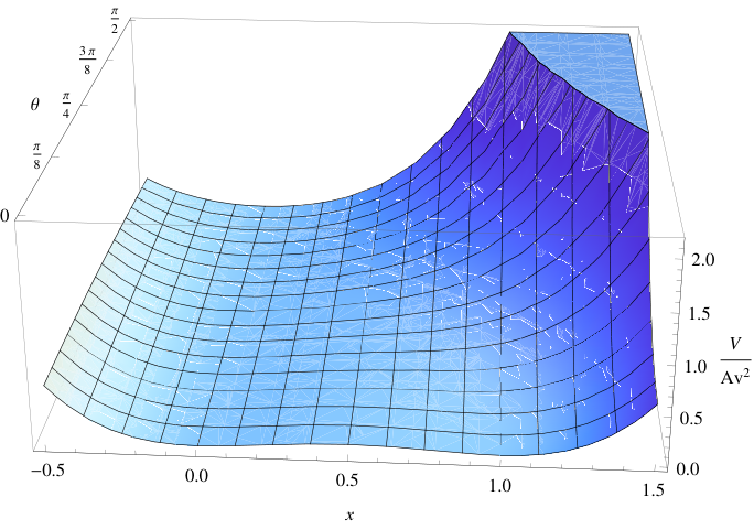
Along the boundary where $\cos\theta=1$, the form of the effective potential (3) is identical to that in the single-field model (1), and the discussion of inflation given in the previous Section goes through unchanged. On the other hand, the potential (3) vanishes along the boundary $x=0$. At any fixed positive value of $x\neq 0$, the potential increases monotonically as $\cos\theta$ decreases from $1\to 0^{+}$. In particular, when $\cos\theta=0$ ($\theta=\pi/2$), the potential is a combination of quadratic and quartic terms with coefficients of the same sign, a scenario that is excluded by the CMB data [3, 2]. A complete discussion of the inflationary possibilities for initial conditions at arbitrary points in the $(x\cos\theta)$ plane lies beyond the scope of this work, but it is clear that, although successful inflation cannot be obtained when $\cos\theta=0$, it would be possible in a neighbourhood of $\cos\theta=1$.

We now discuss how such a Wess-Zumino inflationary model could be combined with the minimal supersymmetric seesaw model. In this case, one would identify the superfield $\Phi$ with the singlet (right-handed) sneutrino superfield. In this case, the quadratic term in (2) would generate $\Delta L=2$ processes (where $L$ is lepton number), corresponding to a Majorana neutrino mass. These processes would conserve $R$ parity. On the other hand, the trilinear term in (2) would generate $\Delta L=3$ processes, which would violate $R$ parity and cause the lightest supersymmetric particle (LSP) to be unstable, in general. However, the rate of $R$ violation would be very small, so the LSP could still provide the astrophysical cold dark matter.

Consider, for example, the case in which the LSP is the gravitino ${\tilde{G}}$. This would have a tree-level coupling to a singlet antisneutrino-neutrino pair. The singlet neutrino would mix with the conventional left-handed neutrino via a Yukawa vertex with a Standard Model Higgs scalar vacuum expectation value divided by the large singlet neutrino mass. On the other hand, the singlet antisneutrino would couple via the the trilinear coupling in (2) to a pair of singlet neutrinos, which would also mix with left-handed neutrinos. This and similar diagrams would give rise to ${\tilde{G}}\to 3\nu$ decay, but at a very low rate, suppressed by several factors of the heavy singlet-neutrino mass scale.

The very precise Planck data [2] are generally consistent with the idea of cosmological inflation (modulo a few well-publicized anomalies), but pose considerable challenges for simple inflationary models. Indeed, no single-field model with a monomial potential $\propto\phi^{n}:n\geq 2$ is comfortably consistent with the data. However, we have shown in this paper that a simple single-field model of the form (1) is highly consistent with the data. Moreover, we have shown that this potential arises very naturally within the simplest single-superfield Wess-Zumino model (2). Finally, we have also shown that this model may be combined with a minimal supersymmetric seesaw model of neutrino masses.

The most important pressure on this model comes from the Planck upper limit on the tensor-to-scalar ratio $r$, and we look forward to future improved constraints on this quantity from CMB polarization data from Planck and other experiments. If the upper limit on $r$ were to be reduced significantly, this would favour variants of the model with larger values of $x_{i}\to 0.5^{-}$, in which case the model might be consistent with the observational constraint on $n_{s}$ for only a more restricted range of $N$.

In the mean time, it would be interesting to explore in more detail the possible predictions of the Wess-Zumino model (2) for $\cos\theta>0$, the possibility of topological inflation, and possible observational signatures of the small violation of $R$ parity that this model would predict if combined with a supersymmetric seesaw model of neutrino masses.

The work of JE and NEM was supported partly by the London Centre for Terauniverse Studies (LCTS), using funding from the European Research Council via the Advanced Investigator Grant 267352. They thank CERN for kind hospitality.

References

- [1] For a recent encyclopedic review see: J. Martin, C. Ringeval and V. Vennin, arXiv:1303.3787 [astro-ph.CO] and references therein.
- [2] For Planck constraints on inflationary models, see P. A. R. Ade et al. [Planck Collaboration], arXiv:1303.5082 [astro-ph.CO]; for a general survey of Planck results including inflation, see P. A. R. Ade et al. [Planck Collaboration], arXiv:1303.5062 [astro-ph.CO].
- [3] E. Komatsu et al. [WMAP Collaboration], Astrophys. J. Suppl. 192, 18 (2011) [arXiv:1001.4538 [astro-ph.CO]]; G. Hinshaw et al., arXiv:1212.5226 [astro-ph.CO].
- [4] L. McAllister, E. Silverstein and A. Westphal, Phys. Rev. D 82 (2010) 046003 [arXiv:0808.0706].
- [5] H. Peiris, R. Easther and R. Flauger, arXiv:1303.2616 [astro-ph.CO].
- [6] E. Silverstein and A. Westphal, Phys. Rev. D 78 (2008) 106003 [arXiv:0803.3085]
- [7] J. Wess and B. Zumino, Nucl. Phys. B 70 (1974) 39.
- [8] H. Murayama, H. Suzuki, T. Yanagida and J.-i. Yokoyama, Phys. Rev. Lett. 70 (1993) 1912 and Phys. Rev. D 50 (1994) 2356 [hep-ph/9311326]; J. R. Ellis, M. Raidal and T. Yanagida, Phys. Lett. B 581 (2004) 9 [hep-ph/0303242].
- [9] A. Kosowsky and M. S. Turner, Phys. Rev. D 52, 1739 (1995) [astro-ph/9504071].
- [10] A. D. Linde, Phys. Lett. B 327 (1994) 208 [astro-ph/9402031].
- [11] A. Vilenkin, Phys. Rev. Lett. 72 (1994) 3137 [hep-th/9402085].
- [12] N. Sakai, H. Shinkai, T. Tachizawa and K.-i. Maeda, Phys. Rev. D 53 (1996) 655 [Erratum-ibid. D 54 (1996) 2981] [gr-qc/9506068].