Fault Tolerance in Distributed Systems using Fused State Machines

Bharath Balasubramanian Affiliation: EDGE Lab, Dept. of Electrical Engineering,
Princeton University,
Engineering Quadrangle, Olden Street,
Princeton, NJ 08544.
Tel.: +1 512 239 8104, . E-mail: bbharath@utexas.edu Vijay K. Garg ^†^†thanks: *This research was supported in part by the NSF Grants CNS-0718990, CNS-0509024, CNS-1115808 and Cullen Trust for Higher Education Endowed Professorship. Affiliation: Parallel and Distributed Systems Laboratory,
Dept. of Electrical and Computer Engineering,
The University of Texas at Austin,
1 University Station, C0803,
Austin, TX 78712-0240.
Tel.: +1 512 471 9424, . E-mail: garg@ece.utexas.edu

Abstract

Replication is a standard technique for fault tolerance in distributed systems modeled as deterministic finite state machines (DFSMs or machines). To correct $f$ crash or $\lfloor f/2\rfloor$ Byzantine faults among $n$ different machines, replication requires $nf$ additional backup machines. We present a solution called fusion that requires just $f$ additional backup machines. First, we build a framework for fault tolerance in DFSMs based on the notion of Hamming distances. We introduce the concept of an ( $f$ , $m$ )-fusion, which is a set of $m$ backup machines that can correct $f$ crash faults or $\lfloor f/2\rfloor$ Byzantine faults among a given set of machines. Second, we present an algorithm to generate an ( $f$ , $f$ )-fusion for a given set of machines. We ensure that our backups are efficient in terms of the size of their state and event sets. Third, we use locality sensitive hashing for the detection and correction of faults that incurs almost the same overhead as that for replication. We detect Byzantine faults with time complexity $O(nf)$ on average while we correct crash and Byzantine faults with time complexity $O(n\rho f)$ with high probability, where $\rho$ is the average state reduction achieved by fusion. Finally, our evaluation of fusion on the widely used MCNC’91 benchmarks for DFSMs show that the average state space savings in fusion (over replication) is 38% (range 0-99%). To demonstrate the practical use of fusion, we describe its potential application to the MapReduce framework. Using a simple case study, we compare replication and fusion as applied to this framework. While a pure replication-based solution requires 1.8 million map tasks, our fusion-based solution requires only 1.4 million map tasks with minimal overhead during normal operation or recovery. Hence, fusion results in considerable savings in state space and other resources such as the power needed to run the backup tasks.

Keywords:

Distributed Systems, Fault Tolerance, Finite State Machines, Coding Theory, Hamming Distances.

1 Introduction

Distributed applications often use deterministic finite state machines (referred to as DFSMs or machines) to model computations such as regular expressions for pattern detection, syntactical analysis of documents or mining algorithms for large data sets. These machines executing on distinct distributed processes are often prone to faults. Traditional solutions to this problem involve some form of replication. To correct $f$ crash faults [25] among $n$ given machines (referred to as primaries), $f$ copies of each primary are maintained [17, 28, 26]. If the backups start from the same initial state as the corresponding primaries and act on the same events, then in the case of faults, the state of the failed machines can be recovered from one of the remaining copies. These backups can also correct $\lfloor f/2\rfloor$ Byzantine faults [18], where the processes lie about the state of the machine, since a majority of truthful machines is always available. This approach, requiring $nf$ total backups, is expensive both in terms of the state space of the backups and other resources such as the power needed to run these backups.

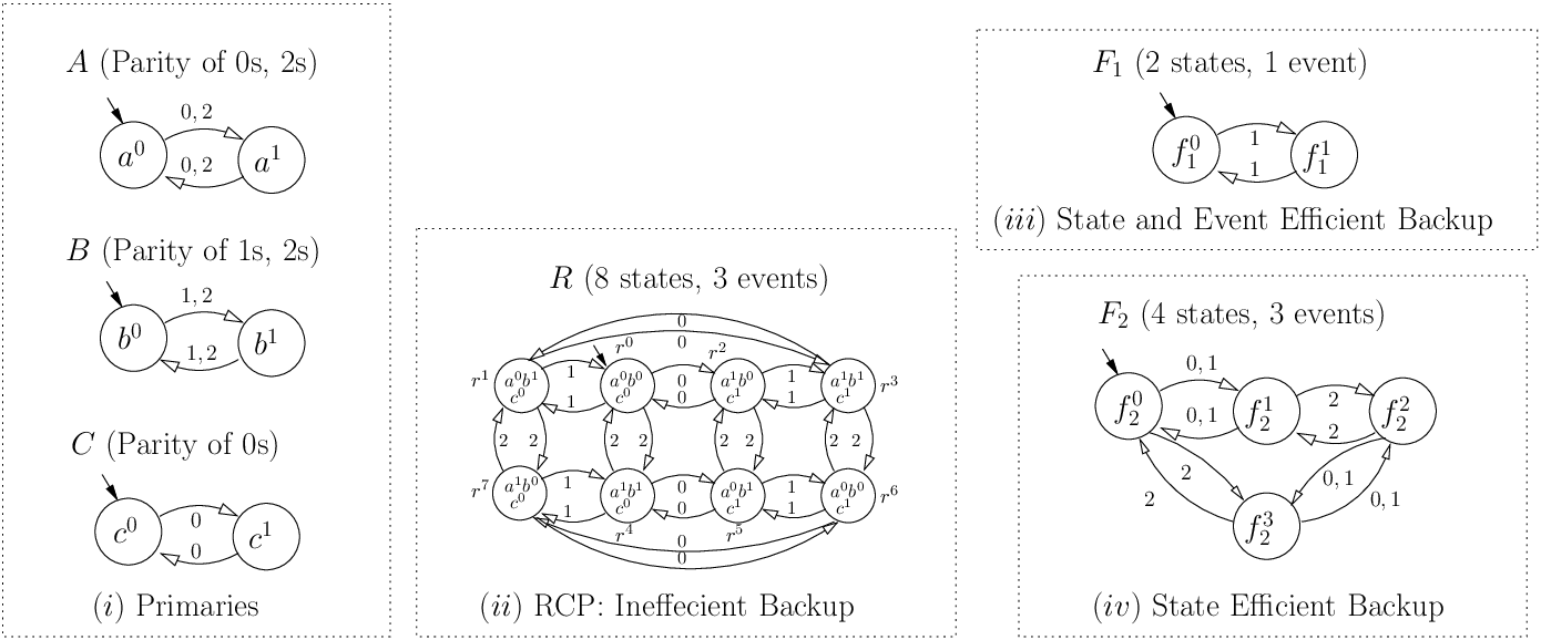
Refer to caption — Figure 1: Correcting one crash fault among $\{A,B,C\}$ using just one additional backup rather than three backups required by replication.

Consider a distributed application that is searching for three different string patterns in a file. These string patterns or regular expressions are usually modeled as DFSMs. Consider the state machines $A$ , $B$ and $C$ shown in Fig. 1. A state machine in our system consists of a finite set of states and a finite set of events. On application of an event, the state machine transitions to the next state based on the state-transition function. For example, machine $A$ in Fig. 1 contains the states $\{a^{0},a^{1}\}$ , events $\{0,2\}$ and the initial state, shown by the dark ended arrow, is $a^{0}$ . The state transitions are shown by the arrows from one state to another. Hence, if $A$ is in state $a^{0}$ and event $0$ is applied to it, then it transitions to state $a^{1}$ . In this example, $A$ checks the parity of $\{0,2\}$ and so, if it is in state $a^{0}$ , then an even number of $0s$ or $2s$ have been applied to the machine and if it is in state $a^{1}$ , then an odd number of the inputs have been applied. Machines $B$ and $C$ check for the parity of $\{1,2\}$ and $\{0\}$ respectively.

To correct one crash fault among these machines, replication requires a copy of each of them, resulting in three backup machines, consuming total state space of eight ( $2^{3}$ ). Another way of looking at replication in DFSMs is by constructing a backup machine that is the reachable cross product or ${RCP}$ (formally defined in section 3.1) of the original machines. As shown in Fig. 1, each state of the ${RCP}$ , denoted by $R$ , is a tuple, in which the elements corresponds to the states of $A$ , $B$ and $C$ respectively. Let each of the machines $A$ , $B$ , $C$ and $R$ start from their initial state. If some event sequence (generated by the client/environment) $0\rightarrow 2\rightarrow 1$ is applied on these machines, then the state of $R$ , $A$ , $B$ and $C$ are $r^{6}=\{a^{0}b^{0}c^{1}\}$ , $a^{0}$ , $b^{0}$ and $c^{1}$ respectively. Here, even if one of the primaries crash, using the state of $R$ , we can determine the state of the crashed primary. Hence, the ${RCP}$ is a valid backup machine.

However, using the ${RCP}$ of the primaries as a backup has two major disadvantages: $(i)$ Given $n$ primaries each containing $O(s)$ states, the number of states in the ${RCP}$ is $O(s^{n})$ , which is exponential in the number of primaries. In Fig. 1, $R$ has eight states. $(ii)$ The event set of the ${RCP}$ is the union of the event sets of the primaries. In Fig. 1 while $A$ , $B$ and $C$ have only two, two and one event respectively in their event sets, $R$ has three events. This translates to increased load on the backup. Can we generate backup machines that are more efficient than the ${RCP}$ in terms of states and events?

Consider $F_{1}$ shown in Fig. 1. If the event sequence $0\rightarrow 0\rightarrow 1\rightarrow 2$ is applied the machines, $A$ , $B$ , $C$ and $F_{1}$ , then they will be in states $a^{1}$ , $b^{0}$ , $c^{0}$ and $f^{1}_{1}$ . Assume a crash fault in $C$ . Given the parity of $1$ s (state of $F_{1}$ ) and the parity of 1s or 2s (state of $B$ ), we can first determine the parity of 2s. Using this, and the parity of 0s or 2s (state of $A$ ), we can determine the parity of 0s (state of $C$ ). Hence, we can determine the state of $C$ as $c^{0}$ using the states of $A$ , $B$ and $F_{1}$ . This argument can be extended to correcting one fault among any of the machines in $\{A,B,C,F_{1}\}$ . This approach consumes fewer backups than replication (one vs. three), fewer states than the ${RCP}$ (two states vs. eight states) and fewer number of events than the ${RCP}$ (one event vs. three events). How can we generate such a backup for any arbitrary set of machines? In Fig. 1, can $F_{1}$ and $F_{2}$ correct two crash faults among the primaries? Further, how do we correct the faults? In this paper, we address such questions through the following contributions:

Framework for Fault Tolerance in DFSMs

We explore the idea of a fault graph and use that to define the minimum Hamming distance [13] for a set of machines. Using this framework, we can specify the exact number of crash or Byzantine faults a set of machines can correct. Further, we introduce the concept of an ( $f$ , $m$ )-fusion which is a set of $m$ machines that can correct $f$ crash faults, detect $f$ Byzantine faults or correct $\lfloor f/2\rfloor$ Byzantine faults. We refer to the machines as fusions or fused backups. In Fig. 1, $F_{1}$ and $F_{2}$ can correct two crash faults among $\{A,B,C\}$ and hence $\{F_{1},F_{2}\}$ is a ( $2$ , $2$ )-fusion of $\{A,B,C\}$ . Replication is just a special case of ( $f$ , $m$ )-fusion where $m=nf$ . We prove properties on the ( $f$ , $m$ )-fusion for a given set of primary machines including lower bounds for the existence of such fusions.

Algorithm to Generate Fused Backup Machines

Given a set of $n$ primaries we present an algorithm that generates an ( $f$ , $f$ )-fusion corresponding to them, i.e., we generate a set of $f$ backup machines that can correct $f$ crash or $\lfloor f/2\rfloor$ Byzantine faults among them. We show that our backups are efficient in terms of: $(i)$ The number of states in each backup $(ii)$ The number of events in each backup $(iii)$ The minimality (defined in section 3.4) of the entire set of backups in terms of states. Further, we show that if our algorithm does not achieve state and event reduction, then no solution with the same number of backups achieves it. Our algorithm has time complexity polynomial in $N$ , where $N$ is the number of states in the ${RCP}$ of the primaries. We present an incremental approach to this algorithm that improves the time complexity by a factor of $O(\rho^{n})$ , where $\rho$ is the average state savings achieved by fusion.

Detection and Correction of Faults

We present a Byzantine detection algorithm with time complexity $O(nf)$ on average, which is the same as the time complexity of detection for replication. Hence, for a system that needs to periodically detect liars, fusion causes no additional overhead. We reduce the problem of fault correction to one of finding points within a certain Hamming distance of a given query point in $n$ -dimensional space and present algorithms to correct crash and Byzantine faults with time complexity $O(n\rho f)$ with high probability (w.h.p). The time complexity for crash and Byzantine correction in replication is $O(f)$ and $O(nf)$ respectively. Hence, for small values of $n$ and $\rho$ , fusion causes almost no overhead for recovery. Table 1 describes the main symbols used in this paper, while Table 2 summarizes the main results in the paper through a comparison with replication.

Table 1: Symbols/Notation used in the paper

$\mathcal{P}$	Set of primaries	$n$	Number of primaries
${RCP}$	Reachable Cross Product	$N$	Number of states in the RCP
$f$	No. of crash faults	$s$	Maximum number of states among primaries
$\mathcal{F}$	Set of fusions/backups	$\rho$	Average State Reduction in fusion
$\Sigma$	Union of primary event-sets	$\beta$	Average Event Reduction in fusion

Table 2: Replication vs. Fusion (Columns 2 and 3 for

f

crash faults, 4 and 5 for

f

Byzantine faults)

	Rep-Crash	Fusion-Crash	Rep-Byz	Fusion-Byz
Number of Backups	$nf$	$f$	$2nf$	$2f$
Backup State Space	$s^{nf}$	$(s^{n}/\rho)^{f}$	$s^{2nf}$	$(s^{n}/\rho)^{2f}$
Average Events/Backup	$\|\Sigma\|/n$	$\|\Sigma\|/\beta$	$\|\Sigma\|/n$	$\|\Sigma\|/\beta$
Fault Detection Time	$O(1)$	$O(1)$	$O(nf)$	$O(nf)$ (on avg.)
Fault Correction Time	$O(f)$	$O(n\rho f)$ w.h.p	$O(nf)$	$O(n\rho f)$ w.h.p
Fault Detection Messages	$O(1)$	$O(1)$	$2nf$	$n+f$
Fault Correction Messages	$f$	$n$	$n+2f$	$n+f$
Backup Generation Time Complexity	$O(nsf)$	$O(s^{n}\|\Sigma\|f/\rho^{n})$	$O(nsf)$	$O(s^{n}\|\Sigma\|f/\rho^{n})$

Fusion-based Grep in the MapReduce Framework

To illustrate the practical use of fusion, we consider its potential application to the grep functionality of the MapReduce framework [8]. The MapReduce framework is a prevalent solution to model large scale distributed computations. The grep functionality is used in many applications that need to identify patterns in huge textual data such as data mining, machine learning and query log analysis. Using a simple case study, we show that a pure replication-based approach for fault tolerance needs 1.8 million map tasks while our fusion-based solution requires only 1.4 million map tasks. Further, we show that our approach causes minimal overhead during normal operation or recovery.

Fusion-based Design Tool and Experimental Evaluation

We provide a Java design tool based on our fusion algorithm, that takes a set of input machines and generates fused backup machines corresponding to them. We evaluate our fusion algorithm on the MCNC’91 [30] benchmarks for DFSMs, that are widely used in the fields of logic synthesis and circuit design. Our results show that the average state space savings in fusion (over replication) is 38% (range 0-99%), while the average event-reduction is 4% (range 0-45%). Further, the average savings in time by the incremental approach for generating the fusions (over the non-incremental approach) is 8%.

In section 2, we specify the system model and assumptions of our work. In section 3 we describe the theory of our backup or fusion machines. Following this, we present algorithms to generate these fusion machines in section 4. In section 5 we present the algorithms for the detection and correction of faults in a system with primary and fusion machines. Sections 6 and 7 deal with the practical aspects and experimental evaluation of fusion. In section 8, we consider potential solutions to this problem, outside the framework of this paper. Section 9 covers the related work in this area. Finally, we summarize our work and discuss future extensions in section 10.

2 Model

The DFSMs in our system execute on separate distributed processes. We assume loss-less FIFO communication links with a strict upper bound on the time taken for message delivery. Clients of the state machines issue the events (or commands) to the concerned primaries and backups. For simplicity, we assume that there is a single client issuing the events to the machines. This along with FIFO links ensures that all machines act on the events in the same relative order. This can be extended to multiple clients using standard total order broadcast mechanisms present in the literature [9, 20].

The execution state of a machine is the current state in which it is executing. Faults in our system are of two types: crash faults, resulting in a loss of the execution state of the machines and Byzantine faults resulting in an arbitrary execution state. We assume that the given set of primary machines cannot correct a single crash fault amongst themselves. When faults are detected by a trusted recovery agent using timeouts (crash faults) or a detection algorithm (Byzantine faults) no further events are sent by any client to these machines. Assuming the machines have acted on the same sequence of events, the recovery agent obtains their states, and recovers the correct execution states of all faulty machines.

3 Framework for Fault Tolerance in DFSMs

In this section, we describe the framework using which we can specify the exact number of crash or Byzantine faults that any set of machines can correct. Further, we introduce the concept of an ( $f$ , $m$ )-fusion for a set of primaries that is a set of machines that can correct $f$ crash faults, detect $f$ Byzantine faults and correct $\lfloor f/2\rfloor$ Byzantine faults.

3.1 DFSMs and their Reachable Cross Product

A DFSM, denoted by ${A}$ , consists of a set of states $X_{A}$ , set of events $\Sigma_{A}$ , transition function $\alpha_{A}:X_{A}\times\Sigma_{A}\rightarrow X_{A}$ and initial state $a^{0}$ . The size of $A$ , denoted by $|A|$ is the number of states in $X_{A}$ . A state, $s\in X_{A}$ , is reachable iff there exists a sequence of events, which, when applied on the initial state $a^{0}$ , takes the machine to state $s$ . Consider any two machines, $A$ $(X_{A},\>\Sigma_{A},\>\alpha_{A},\>a^{0})$ and $B$ $(X_{B},\>\Sigma_{B},\>\alpha_{B},\>b^{0})$ . Now construct another machine which consists of all the states in the product set of $X_{A}$ and $X_{B}$ with the transition function $\alpha^{\prime}(\{a,b\},\sigma)=\{\alpha_{A}(a,\sigma),\alpha_{B}(b,\sigma)\}$ for all $\{a,b\}\in X_{A}\times X_{B}$ and $\sigma\in\Sigma_{A}\cup\Sigma_{B}$ . This machine $(X_{A}\times X_{B},\>\Sigma_{A}\cup\Sigma_{B},\>\alpha^{\prime},\>\{a^{0},b^{0}\})$ may have states that are not reachable from the initial state $\{a^{0},b^{0}\}$ . If all such unreachable states are pruned, we get the reachable cross product of $A$ and $B$ . In Fig. 1, $R$ is the reachable cross product of $A$ , $B$ and $C$ . Throughout the paper, when we just say ${RCP}$ , we refer to the reachable cross product of the set of primary machines. Given a set of primaries, the number of states in its ${RCP}$ is denoted by $N$ and its event set, which is the union of the event sets of the primaries is denoted by $\Sigma$ .

As seen in section 1, given the state of the ${RCP}$ , we can determine the state of each of the primary machines and vice versa. However, the ${RCP}$ has states exponential in $n$ and an event set that is the union of all primary event sets. Can we generate machines that contains fewer states and events than the ${RCP}$ ? In the following section, we first define the notion of order and the ‘less than or equal to’ $(\leq)$ relation among machines.

3.2 Order Among Machines and their Closed Partition Lattice

Consider a DFSM, $A=(X_{A},\Sigma,\alpha_{A},x^{0}_{A})$ . A partition $P$ , on the state set $X_{A}$ of $A$ is the set $\{B_{1},\ldots,B_{k}\}$ , of disjoint subsets of the state set $X_{A}$ , such that $\bigcup^{k}_{i=1}B_{i}=X_{A}$ and $B_{i}\cap B_{j}=\phi$ for $i\neq j$ [19]. An element $B_{i}$ of a partition is called a block. A partition, $P$ , is said to be closed if each event, $\sigma\in\Sigma$ , maps a block of $P$ into another block. A closed partition $P$ , corresponds to a distinct machine. Given any machine $A$ , we can partition its state space such that the transition function $\alpha_{A}$ , maps each block of the partition to another block for all events in $\Sigma_{A}$ [14, 19].

In other words, we combine the states of $A$ to generate machines that are consistent with the transition function. We refer to the set of all such closed partitions as the closed partition set of $A$ . In this paper, we discuss the closed partitions corresponding to the ${RCP}$ of the primaries. In Fig. 2, we show the closed partition set of the ${RCP}$ of $\{A,B,C\}$ (labeled $R$ ). Consider machine $M_{2}$ in Fig. 2, generated by combining the states $r^{0}$ and $r^{2}$ of $R$ . Note that, on event 1, $r^{0}$ transitions to $r^{1}$ and $r^{2}$ transitions to $r^{3}$ . Hence, we need to combine the states $r^{1}$ and $r^{3}$ . Continuing this procedure, we obtain the combined states in $M_{2}$ . Hence, we have reduced the ${RCP}$ to generate $M$ . By combining different pairs of states and by further reducing the machines thus formed, we can construct the entire closed partition set of $R$ .

We can define an order ( $\leq$ ) among any two machines $P$ and $Q$ in this set as follows: $P\leq Q$ , if each block of $Q$ is contained in a block of $P$ (shown by an arrow from $P$ to $Q$ ). Intuitively, given the state of $Q$ we can determine the state of $P$ . Machines $P$ and $Q$ are incomparable, i.e., $P||Q$ , if $P\not<Q$ and $Q\not<P$ . In Fig. 2, $F_{1}<M_{2}$ , while $M_{1}||M_{2}$ . It can be seen that the set of all closed partitions corresponding to a machine, form a lattice under the $\leq$ relation [14]. We saw in section 3.1 that given the state of the primaries, we can determine the state of the ${RCP}$ and vice versa. Hence, the primary machines are always part of the closed partition set of the ${RCP}$ (see $A$ , $B$ and $C$ in Fig. 2).

Among the machines shown in Fig. 2, some of them, like $F_{2}$ (4 states, 3 events) have reduced states, while some like $M_{1}$ (4 states, 2 events) and $F_{1}$ (2 states, 1 event) have both reduced states and events as compared to $R$ (8 states, 3 events). Which among these machines can act as backups? In the following section, we describe the concept of fault graphs and their Hamming distances to answer this question.

3.3 Fault Graphs and Hamming Distances

We begin with the idea of a fault graph of a set of machines $\mathcal{M}$ , for a machine $T$ , where all machines in $\mathcal{M}$ are less than or equal to $T$ . This is a weighted graph and is denoted by $G(T,\mathcal{M})$ . The fault graph is an indicator of the capability of the set of machines in $\mathcal{M}$ to correctly identify the current state of $T$ . As described in the previous section, since all the machines in $\mathcal{M}$ are less than or equal to $T$ , the set of states of any machine in $\mathcal{M}$ corresponds to a closed partition of the set of states of $T$ . Hence, given the state of $T$ , we can determine the state of all the machines in $\mathcal{M}$ and vice versa.

Definition 1

(Fault Graph) Given a set of machines $\mathcal{M}$ and a machine $T=(X_{T},\Sigma_{T},\alpha_{T},t^{0})$ such that $\forall M\in\mathcal{M}:M\leq T$ , the fault graph $G(T,\mathcal{M})$ is a fully connected weighted graph where,

•

Every node of the graph corresponds to a state in $X_{T}$
•

The weight of the edge $(t^{i},t^{j})$ between two nodes, where $t^{i},t^{j}\in X_{T}$ , is the number of machines in $\mathcal{M}$ that have states $t^{i}$ and $t^{j}$ in distinct blocks

We construct the fault graph $G(R,\{A\})$ , referring to Fig. 2. $A$ has two states, $a^{0}=\{r^{0},r^{1},r^{5},r^{6}\}$ and $a^{1}=\{r^{2},r^{3},r^{4},r^{7}\}$ . Given just the current state of $A$ , it is possible to determine if $R$ is in state $r^{0}$ or $r^{2}$ (exact) or one of $r^{0}$ and $r^{1}$ (ambiguity). Here, $A$ distinguishes between the $(r^{0},r^{2})$ but not between $(r^{0},r^{1})$ . Hence, in the fault graph $G(R,\{A\})$ in Fig. 3 $(i)$ , the edge $(r^{0},r^{2})$ has weight one, while $(r^{0},r^{1})$ has weight zero. A machine $M\in\mathcal{M}$ , is said to cover an edge $(t^{i},t^{j})$ if $t^{i}$ and $t^{j}$ lie in separate blocks of $M$ , i.e., $M$ separates the states $t^{i}$ and $t^{j}$ . In Fig. 2, $A$ covers $(r^{0},r^{2})$ . In Fig. 9 and 10 of the Appendix, we show an example of the closed partition set and fault graphs for a different set of primaries.

Given the states of $|\mathcal{M}|-x$ machines in $|\mathcal{M}|$ , it is always possible to determine if $T$ is in state $t^{i}$ or $t^{j}$ iff the weight of the edge $(t^{i},t^{j})$ is greater than $x$ . Consider the graph shown in Fig. 3 $(ii)$ . Given the state of any two machines in $\{A,B,C\}$ , we can determine if $R$ is in state $r^{0}$ or $r^{2}$ , since the weight of that edge is greater than one, but cannot do the same for the edge $(r^{0},r^{1})$ , since the weight of the edge is one. In coding theory [7, 24], the concept of Hamming distance [13] is widely used to specify the fault tolerance of an erasure code. If an erasure code has minimum Hamming distance greater than $d$ , then it can correct $d$ erasures or $\lfloor d/2\rfloor$ errors. To understand the fault tolerance of a set of machines, we define a similar notion of distances for the fault graph.

Definition 2

(distance) Given a set of machines $\mathcal{M}$ and their reachable cross product $T$ $(X_{T},\Sigma_{T},\alpha_{T},t^{0})$ , the distance between any two states $t_{i},t_{j}\in X_{T}$ , denoted by $d(t_{i},t_{j})$ , is the weight of the edge $(t_{i},t_{j})$ in the fault graph $G(T,\mathcal{M})$ . The least distance in $G(T,\mathcal{M})$ is denoted by $d_{min}(T,\mathcal{M})$ .

Given a fault graph, $G(T,\mathcal{M})$ , the smallest distance between the nodes in the fault graph specifies the fault tolerance of $\mathcal{M}$ . Consider the graph, $G(R,\{A,B,C,F_{1},F_{2}\})$ , shown in Fig. 3 $(v)$ . Since the smallest distance in the graph is three, we can remove any two machines from $\{A,B,C,F_{1},F_{2}\}$ and still regenerate the current state of $R$ . As seen before, given the state of $R$ , we can determine the state of any machine less than $R$ . Therefore, the set of machines $\{A,B,C,F_{1},F_{2}\}$ can correct two crash faults.

Theorem 3.1

A set of machines $\mathcal{M}$ , can correct up to $f$ crash faults iff $d_{min}(T,\mathcal{M})>f$ , where $T$ is the reachable cross-product of all machines in $\mathcal{M}$ .

Proof

$(\Rightarrow)$ Given that $d_{min}(T,\mathcal{M})>f$ , we show that any $\mathcal{M}-f$ machines from $\mathcal{M}$ can accurately determine the current state of $T$ , thereby recovering the state of the crashed machines. Since $d_{min}(T,\mathcal{M})>f$ , by definition, at least $f+1$ machines separate any two states of $X_{T}$ . Hence, for any pair of states $(t_{i},t_{j})\in X_{T}$ , even after $f$ crash failures in $\mathcal{M}$ , at least one machine remains that can distinguish between $t_{i}$ and $t_{j}$ . This implies that it is possible to accurately determine the current state of $T$ by using any $\mathcal{M}-f$ machines from $\mathcal{M}$ .

$(\Leftarrow)$ Given that $d_{min}(T,\mathcal{M})\leq f$ , we show that the system cannot correct $f$ crash faults. The condition $d_{min}(T,\mathcal{M})\leq f$ implies that there exists states $t_{i}$ and $t_{j}$ in $G(T,\mathcal{M})$ separated by distance $k$ , where $k\leq f$ . Hence there exist exactly $k$ machines in $\mathcal{M}$ that can distinguish between states $t_{i},t_{j}\in X_{T}$ . Assume that all these $k$ machines crash (since $k\leq f$ ) when $T$ is in either $t_{i}$ or $t_{j}$ . Using the states of the remaining machines in $\mathcal{M}$ , it is not possible to determine whether $T$ was in state $t_{i}$ or $t_{j}$ . Therefore, it is not possible to exactly regenerate the state of any machine in $\mathcal{M}$ using the remaining machines.

Byzantine faults may include machines which lie about their state. Consider the machines $\{A,B,C,F_{1},F_{2}\}$ shown in Fig. 2. From Fig. 3 $(v)$ , Let the execution states of the machines $A$ , $B$ , $C$ , $F_{1}$ and $F_{2}$ be

a^{0}=\{r^{0},r^{1},r^{5},r^{6}\},b^{1}=\{r^{1},r^{3},r^{4},r^{5}\},c^{0}=\{r^{0},r^{1},r^{4},r^{7}\}

f_{1}^{0}=\{r^{0},r^{2},r^{4},r^{5}\},f_{2}^{0}=\{r^{0},r^{3}\},

respectively. Since $r^{0}$ appears four times (greater than majority) among these states, even if there is one liar we can determine that $R$ is in state $r^{0}$ . But if $R$ is in state $r^{0}$ , then $B$ must have been in state $b^{0}$ which contains $r^{0}$ . So clearly, $B$ is lying and its correct state is $b^{1}$ . Here, we can determine the correct state of the liar, since $d_{min}(R,\{A,B,C,F_{1},F_{2}\})=3$ , and the majority of machines distinguish between all pairs of states.

Theorem 3.2

A set of machines $\mathcal{M}$ , can correct up to $f$ Byzantine faults iff $d_{min}(T,\mathcal{M})>2f$ , where $T$ is the reachable cross-product of all machines in $\mathcal{M}$ .

Proof

$(\Rightarrow)$ Given that $d_{min}(T,\mathcal{M})>2f$ , we show that any $\mathcal{M}-f$ correct machines from $\mathcal{M}$ can accurately determine the current state of $T$ in spite of $f$ liars. Since $d_{min}(T,\mathcal{M})>2f$ , at least $2f+1$ machines separate any two states of $X_{T}$ . Hence, for any pair of states $t_{i},t_{j}\in X_{T}$ , after $f$ Byzantine failures in $\mathcal{M}$ , there will always be at least $f+1$ correct machines that can distinguish between $t_{i}$ and $t_{j}$ . This implies that it is possible to accurately determine the current state of $T$ by simply taking a majority vote.

$(\Leftarrow)$ Given that $d_{min}(T,\mathcal{M})\leq 2f$ , we show that the system cannot correct $f$ Byzantine faults. $d_{min}(T,\mathcal{M})\leq 2f$ implies that there exists states $t_{i},t_{j}\in X_{T}$ separated by distance $k$ , where $k\leq 2f$ . If $f$ among these $k$ machines lie about their state, we have only $k-f$ correct machines remaining. Since, $k-f\leq f$ , it is impossible to distinguish the liars from the truthful machines and regenerate the correct state of $T$ .

In this paper, we are concerned only with the fault graph of machines w.r.t the ${RCP}$ of the primaries $\mathcal{P}$ . For notational convenience, we use $G(\mathcal{M})$ instead of $G({RCP},\mathcal{M})$ and $d_{min}(\mathcal{M})$ instead of $d_{min}({RCP},\mathcal{M})$ . From theorems 3.1 and 3.2, it is clear that a set of $n$ machines $\mathcal{P}$ , can correct $(d_{min}(\mathcal{P})-1)$ crash faults and $\lfloor(d_{min}(\mathcal{P})-1)/2\rfloor$ Byzantine faults. Henceforth, we only consider backup machines less than or equal to the ${RCP}$ of the primaries. In the following section, we describe the theory of such backup machines.

3.4 Theory of ( $f$ , $m$ )-fusion

To correct faults in a given set of machines, we need to add backup machines so that the fault tolerance of the system (original set of machines along with the backups) increases to the desired value. To simplify the discussion, in the remainder of this paper, unless specified otherwise, we mean crash faults when we simply say faults. Given a set of $n$ machines $\mathcal{P}$ , we add $m$ backup machines $\mathcal{F}$ , each less than or equal to the ${RCP}$ , such that the set of machines in $\mathcal{P\cup F}$ can correct $f$ faults. We call the set of $m$ machines in $\mathcal{F}$ , an ( $f$ , $m$ )-fusion of $\mathcal{P}$ . From theorem 3.1, we know that, $d_{min}(\mathcal{P\cup F})>f$ .

Definition 3

(Fusion) Given a set of $n$ machines $\mathcal{P}$ , we refer to the set of $m$ machines $\mathcal{F}$ , as an ( $f$ , $m$ )-fusion of $\mathcal{P}$ , if $d_{min}(\mathcal{P\cup F})>f$ .

Any machine belonging to $\mathcal{F}$ is referred to as a fused backup or just a fusion. Consider the set of machines, $\mathcal{P}=\{A,B,C\}$ , shown in Fig. 1. From Fig. 3 $(ii)$ , $d_{min}(\{A,B,C\})=1$ . Hence the set of machines $\mathcal{P}$ , cannot correct a single fault. To generate a set of machines $\mathcal{F}$ , such that, $\mathcal{P\cup F}$ can correct two faults, consider Fig. 3 $(v)$ . Since $d_{min}(\{A,B,C,F_{1},F_{2}\})=3$ , $\{A,B,C,F_{1},F_{2}\}$ can correct two faults. Hence, $\{F_{1},F_{2}\}$ is a ( $2$ , $2$ )-fusion of $\{A,B,C\}$ . Note that the set of machines in $\{A,A,B,B,C,C\}$ , i.e., replication, is a ( $2$ , $6$ )-fusion of $\{A,B,C\}$ .

Any machine in the set $\{A,B,C,F_{1},F_{2}\}$ can at most contribute a value of one to the weight of any edge in the graph $G(\{A,B,C,F_{1},F_{2}\})$ . Hence, even if we remove one of the machines, say $F_{2}$ , from this set, $d_{min}(\{A,B,C,F_{1}\})$ is greater than one. So $\{F_{1}\}$ is an ( $1$ , $1$ )-fusion of $\{A,B,C\}$ .

Theorem 3.3

(Subset of a Fusion) Given a set of $n$ machines $\mathcal{P}$ , and an ( $f$ , $m$ )-fusion $\mathcal{F}$ , corresponding to it, any subset $\mathcal{F}^{\prime}\subseteq\mathcal{F}$ such that $|\mathcal{F}^{\prime}|=m-t$ is a ( $f-t$ , $m-t$ )-fusion when $t\leq min(f,m)$ .

Proof

Since, $\mathcal{F}$ is an ( $f$ , $m$ )-fusion of $\mathcal{P}$ , $d_{min}(\mathcal{P\cup F})>f$ . Any machine, $F\in\mathcal{F}$ , can at most contribute a value of one to the weight of any edge of the graph, $G(\mathcal{P\cup F})$ . Therefore, even if we remove $t$ machines from the set of machines in $\mathcal{F}$ , $d_{min}(\mathcal{P\cup F})>f-t$ . Hence, for any subset $\mathcal{F}^{\prime}\subseteq\mathcal{F}$ , of size $m-t$ , $d_{min}(\mathcal{P\cup F^{\prime}})>f-t$ . This implies that $\mathcal{F^{\prime}}$ is an ( $f-t$ , $m-t$ )-fusion of $\mathcal{P}$ .

It is important to note that the converse of this theorem is not true. In Fig. 2, while $\{M_{2}\}$ and $\{F_{1}\}$ are ( $1$ , $1$ )-fusions of $\{A,B,C\}$ , since $d_{min}(\{A,B,C,M_{2},F_{1}\})=2$ , $\{M_{2},F_{1}\}$ is not a ( $2$ , $2$ )-fusion of $\{A,B,C\}$ . We now consider the existence of an ( $f$ , $m$ )-fusion for a given set of machines $\mathcal{P}$ . Consider the existence of a ( $2$ , $1$ )-fusion for $\{A,B,C\}$ in Fig. 2. From Fig. 3 $(ii)$ , $d_{min}(\{A,B,C\})=1$ . Clearly, $R$ covers each pair of edges in the fault graph. Even if we add $R$ to this set, from Fig. 3 $(iii)$ , $d_{min}(\{A,B,C,R\})<3$ . Hence, there cannot exist a ( $2$ , $1$ )-fusion for $\{A,B,C\}$ .

Theorem 3.4

(Existence of Fusions) Given a set of $n$ machines $\mathcal{P}$ , there exists an ( $f$ , $m$ )-fusion of $\mathcal{P}$ iff $m+d_{min}(\mathcal{P})>f$ .

Proof

$(\Rightarrow)$ Assume that there exists an ( $f$ , $m$ )-fusion $\mathcal{F}$ for the given set of machines $\mathcal{P}$ . Since, $\mathcal{F}$ is an ( $f$ , $m$ )-fusion fusion of $\mathcal{P}$ , $d_{min}(\mathcal{P\cup F})>f$ . The $m$ machines in $\mathcal{F}$ , can at most contribute a value of $m$ to the weight of each edge in $G(\mathcal{P\cup F})$ . Hence, $m+d_{min}(\mathcal{P})$ has to be greater than $f$ .

$(\Leftarrow)$ Assume that $m+d_{min}(\mathcal{P})>f$ . Consider a set of $m$ machines $\mathcal{F}$ , containing $m$ copies of the ${RCP}$ . These copies contribute exactly $m$ to the weight of each edge in $G(\mathcal{P\cup F})$ . Since, $d_{min}(\mathcal{P})>f-m$ , $d_{min}(\mathcal{P\cup F})>f$ . Hence, $\mathcal{F}$ is an ( $f$ , $m$ )-fusion of $\mathcal{P}$ .

Given a set of machines, we now define an order among ( $f$ , $m$ )-fusions corresponding to them.

Definition 4

(Order among ( $f$ , $m$ )-fusions) Given a set of $n$ machines $\mathcal{P}$ , an ( $f$ , $m$ )-fusion $\mathcal{F}=\{F_{1},..F_{m}\}$ , is less than another ( $f$ , $m$ )-fusion $\mathcal{G}$ , i.e, $\mathcal{F}<\mathcal{G}$ , iff the machines in $\mathcal{G}$ can be ordered as $\{G_{1},G_{2},..G_{m}\}$ such that $\forall 1\leq i\leq m:(F_{i}\leq G_{i})\wedge(\exists j:F_{j}<G_{j})$ .

An ( $f$ , $m$ )-fusion $\mathcal{F}$ is minimal, if there exists no ( $f$ , $m$ )-fusion $\mathcal{F}^{\prime}$ , such that, $\mathcal{F}^{\prime}<\mathcal{F}$ . It can be seen that,

d_{min}(\{A,B,C,M_{2},F_{2}\})=3,

and hence, $\mathcal{F}^{\prime}=\{M_{2},F_{2}\}$ is a ( $2$ , $2$ )-fusion of $\{A,B,C\}$ . We have seen that $\mathcal{F}=\{F_{1},F_{2}\}$ , is a ( $2$ , $2$ )-fusion of $\{A,B,C\}$ . From Fig. 2, since $F_{1}<M_{2}$ , $\mathcal{F}<\mathcal{F}^{\prime}$ . In Fig. 2, since $R_{\bot}$ cannot be a fusion for $\{A,B,C\}$ , there exists no ( $2$ , $2$ )-fusion less than $\{F_{1},F_{2}\}$ . Hence, $\{F_{1},F_{2}\}$ is a minimal ( $2$ , $2$ )-fusion of $\{A,B,C\}$ .

We now prove a property of the fusion machines that is crucial for practical applications. Consider a set of primaries $\mathcal{P}$ and an ( $f$ , $m$ )-fusion $\mathcal{F}$ corresponding to it. The client sends updates addressed to the primaries to all the backups as well. We show that events or inputs that belong to distinct set of primaries, can be received in any order at each of the fused backups. This eliminates the need for synchrony at the backups.

Consider a fusion $F\in\mathcal{F}$ . Since the states of $F$ are essentially partitions of the state set of the ${RCP}$ , the state transitions of $F$ are defined by the state transitions of the ${RCP}$ . For example, machine $M_{1}$ in Fig. 2 transitions from $\{r^{0},r^{2}\}$ to $\{r^{1},r^{3}\}$ on event 1, because $r^{0}$ and $r^{2}$ transition to $r^{1}$ and $r^{3}$ respectively on event 1. Hence, if we show that the state of the ${RCP}$ is independent of the order in which it receives events addressed to different primaries, then the same applies to the fusions.

Theorem 3.5

(Commutativity) The state of a fused backup after acting on a sequence of events, is independent of the order in which the events are received, as long as the events belong to distinct sets of primaries.

Proof

We first prove the theorem for the ${RCP}$ , which is also a valid fused backup. Let the set of primaries be $\mathcal{P}=\{P_{1}\ldots P_{n}\}$ . Consider an event $e_{i}$ that belongs to the set of primaries $\mathcal{S}_{i}\subseteq\mathcal{P}$ . If the ${RCP}$ is in state $r$ , its next state transition on event $e_{i}$ depends only on the transition functions of the primaries in $\mathcal{S}_{i}$ . Hence, the state of the ${RCP}$ after acting on two events $e_{a}$ and $e_{b}$ is independent of the order in which these events are received by the ${RCP}$ , as long as $\mathcal{S}_{a}\cup\mathcal{S}_{b}=\phi$ . The proof of the theorem follows directly from this.

So far, we have presented the framework to understand fault tolerance among machines. Given a set of machines, we can determine if they are a valid set of backups by constructing the fault graph of those machines. In the following section, we present a technique to generate such backups automatically.

4 Algorithm to Generate Fused Backup Machines

genFusion Input: Primaries $\mathcal{P}$ , faults $f$ , state-reduction parameter $\bigtriangleup s$ ,
event-reduction parameter $\bigtriangleup e$ ;
Output: ( $f$ , $f$ )-fusion of $\mathcal{P}$ ;
$\mathcal{F}\leftarrow\{\}$ ;
//Outer Loop
for $(i=1$ to $f)$
Identify weakest edges in fault graph $G(\mathcal{P}\cup\mathcal{F})$ ;
$\mathcal{M}\leftarrow\{RCP(\mathcal{P})\}$ ;
//State Reduction Loop
for ( $j=1$ to $\bigtriangleup s$ )
$\mathcal{S}\leftarrow\{\}$ ;
for $(M\in\mathcal{M})$
$\mathcal{S}=\mathcal{S}\cup\emph{reduceState}(M)$ ;
$\mathcal{M}$ = All machines in $\mathcal{S}$ that increment $d_{min}(\mathcal{P}\cup\mathcal{F})$ ;
//Event Reduction Loop
for ( $j=1$ to $\bigtriangleup e$ )
$\mathcal{E}\leftarrow\{\}$ ;
for $(M\in\mathcal{M})$
$\mathcal{E}=\mathcal{E}\cup\emph{reduceEvent}(M)$ ;
$\mathcal{M}$ = All machines in $\mathcal{E}$ that increment $d_{min}(\mathcal{P}\cup\mathcal{F})$ ;
//Minimality Loop
$M\leftarrow$ Any machine in $\mathcal{M}$ ;
while (all states of $M$ have not been combined)
$\mathcal{C}\leftarrow\emph{reduceState}(M)$ ;
$M$ = Any machine in $\mathcal{C}$ that increments $d_{min}(\mathcal{P}\cup\mathcal{F})$ ;
$\mathcal{F}\leftarrow\{M\}\bigcup\mathcal{F}$ ;
return $\mathcal{F}$ ; reduceState Input: Machine $P$ with state set $X_{P}$ , event set $\Sigma_{P}$
and transition function $\alpha_{P}$ ;
Output: Largest Machines $<P$ with $\leq|X_{P}|-1$ states;
$\mathcal{B}=\{\}$ ;
for $(s_{i},s_{j}\in X_{P})$
//combine states $s_{i}$ and $s_{j}$
Set of states, $X_{B}=X_{P}$ with $(s_{i},s_{j})$ combined;
$\mathcal{B}=\mathcal{B}\cup\{$ Largest machine consistent with $X_{B}\}$ ;
return largest incomparable machines in $\mathcal{B}$ ;

reduceEvent
Input: Machine $P$ with state set $X_{P}$ , event set $\Sigma_{P}$
and transition function $\alpha_{P}$ ;
Output: Largest Machines $<P$ with $\leq|\Sigma_{P}|-1$ events;
$\mathcal{B}=\{\}$ ;
for $(\sigma\in\Sigma_{P})$
Set of states, $X_{B}=X_{P}$ ;
//combine states to self-loop on $\sigma$
for ( $s\in X_{B}$ )
$s=s\cup\alpha_{P}(s,\sigma)$ ;
$\mathcal{B}=\mathcal{B}\cup\{$ Largest machine consistent with $X_{B}\}$ ;
return largest incomparable machines in $\mathcal{B}$ ;

Figure 4: Algorithm to generate an (

f

f

)-fusion for a given set of primaries

\mathcal{P}

. Note that, we use the terms largest, incomparable w.r.t the order defined in section 3.2.

Given a set of $n$ primaries $\mathcal{P}$ , we present an algorithm to generate an ( $f$ , $f$ )-fusion $\mathcal{F}$ of $\mathcal{P}$ . The number of faults to be corrected, $f$ , is an input parameter based on the system’s requirements. The algorithm also takes as input two parameters $\bigtriangleup s$ and $\bigtriangleup e$ and ensures (if possible) that each machine in $\mathcal{F}$ has at most $(N-\bigtriangleup s)$ states and at most $(|\Sigma|-\bigtriangleup e)$ events, where $N$ and $\Sigma$ are the number of states and events in the ${RCP}$ . Further, we show that $\mathcal{F}$ is a minimal fusion of $\mathcal{P}$ . The algorithm has time complexity polynomial in $N$ .

The genFusion algorithm executes $f$ iterations and in each iteration adds a machine to $\mathcal{F}$ that increases $d_{min}(\mathcal{P\cup F})$ (referred to as $d_{min}$ ) by one. At the end of $f$ iterations, $d_{min}$ increases to $f+1$ and hence $\mathcal{P\cup F}$ can correct $f$ faults. The algorithm ensures that the backup selected in each iteration is optimized for states and events. In the following paragraphs, we explain the genFusion algorithm in detail, followed by an example to illustrate its working.

In each iteration of the genFusion algorithm (Outer Loop), we first identify the set of weakest edges in $\mathcal{P\cup F}$ and then find a machine that covers these edges, thereby increasing $d_{min}$ by one. We start with the ${RCP}$ , since it always increases $d_{min}$ . The ‘State Reduction Loop’ and the ‘Event Reduction Loop’ successively reduce the states and events of the ${RCP}$ . Finally the ‘Minimality Loop’ searches as deep into the closed partition set of the ${RCP}$ as possible for a reduced state machine, without explicitly constructing the lattice.

State Reduction Loop: This loop uses the reduceState algorithm in Fig. 4 to iteratively generate machines with fewer states than the ${RCP}$ that increase $d_{min}$ by one. The reduceState algorithm, takes as input, a machine $P$ and generates a set of machines in which at least two states of $P$ are combined. For each pair of states $s_{i},s_{j}$ in $X_{P}$ , the reduceState algorithm, first creates a partition of blocks in which $(s_{i},s_{j})$ are combined and then constructs the largest machine consistent with this partition. Note that, ‘largest’ is based on the order specified in section 3.2. This procedure is repeated for all pairs in $X_{P}$ and the largest incomparable machines among them are returned. At the end of $\bigtriangleup s$ iterations of the state reduction loop, we generate a set of machines $\mathcal{M}$ each of which increases $d_{min}$ by one and contains at most $(N-\bigtriangleup s)$ states, if such machines exist.

Event Reduction Loop: Starting with the state reduced machines in $\mathcal{M}$ , the event reduction loop uses the reduceEvent algorithm in Fig. 4 to generate reduced event machines that increase $d_{min}$ by one. The reduceEvent algorithm, takes as input, a machine $P$ and generates a set of machines that contain at least one event less than $\Sigma_{P}$ . To generate a machine less than any given input machine $P$ , that does not contain an event $\sigma$ in its event set, the reduceEvent algorithm combines the states such that they loop onto themselves on $\sigma$ . The algorithm then constructs the largest machine that contains these states in the combined form. This machine, in effect, ignores $\sigma$ . This procedure is repeated for all events in $\Sigma_{P}$ and the largest incomparable machines among them are returned. At the end of $\bigtriangleup e$ iterations of the event reduction loop, we generate a set of machines $\mathcal{M}$ each of which increases $d_{min}$ by one and contains at most $(N-\bigtriangleup s)$ states and at most $(|\Sigma|-\bigtriangleup e)$ events, if such machines exist. ¹¹ 1 In Appendix A, we present the concept of the event-based decomposition of machines to replace a given machine $A$ with a set of machines that contain fewer events than $\Sigma_{A}$ .

Minimality Loop: This loop picks any machine $M$ among the state and event reduced machines in $\mathcal{M}$ and uses the reduceState algorithm iteratively to generate a machine less than $M$ that increases $d_{min}$ by one until no further state reduction is possible i.e., all the states of $M$ have been combined. Unlike the state reduction loop (which also uses the reduceState algorithm), in the minimality loop we never exhaustively explore all state reduced machines. After each iteration of the minimality loop, we only pick one machine that increases $d_{min}$ by one.

Note that, in all three of these inner loops, if in any iteration, no reduction is achieved, then we simply exit the loop with the machines generated in the previous iteration. We use the example in Fig. 2 with $\mathcal{P}=\{A,B,C\},f=2,\bigtriangleup s=1$ and $\bigtriangleup e=1$ , to explain the genFusion algorithm. Since $f=2$ , there are two iterations of the outer loop and in each iteration we generate one machine. Consider the first iteration of the outer loop. Initially, $\mathcal{F}$ is empty and we need to add a machine that covers the weakest edges in $G(\{A,B,C\})$ .

To identify the weakest edges, we need to identify the mapping between the states of the ${RCP}$ and the states of the primaries. For example, in Fig. 2, we need to map the states of the ${RCP}$ to $A$ . The starting states are always mapped to each other and hence $r^{0}$ is mapped to $a^{0}$ . Now $r^{0}$ on event $0$ transitions to $r^{2}$ , while $a^{0}$ on event $0$ transitions to $a^{1}$ . Hence, $r^{2}$ is mapped to $a^{1}$ . Continuing this procedure for all states and events, we obtain the mapping shown, i.e, $a^{0}=\{r^{0},r^{1},r^{5},r^{6}\}$ and $a^{1}=\{r^{2},r^{3},r^{4},r^{7}\}$ . Following this procedure for all primaries, we can identify the weakest edges in $G(\{A,B,C\})$ (Fig. 3 $(ii)$ ). In Fig. 2, $M_{1}$ , $M_{2}$ and $F_{2}$ are some of the largest incomparable machines that contain at least one state less than the ${RCP}$ (the entire set is too large to be enumerated here). All three of these machines increase $d_{min}$ and at the end of the one and only iteration of the state reduction loop, $\mathcal{M}$ will contain at least these three machines.

The event reduction loop tries to find machines with fewer events than the machines in $\mathcal{M}$ . For example, to generate a machine less than $M_{2}$ that does not contain, say event 2, the reduceEvent algorithm combines the blocks of $M_{2}$ such that they do not transition on event 2. Hence, $\{r^{0},r^{2}\}$ in $M_{2}$ is combined with $\{r^{4},r^{5}\}$ and $\{r^{1},r^{3}\}$ is combined with $\{r^{6},r^{7}\}$ to generate machine $F_{1}$ that does not act on event 2. The only machine less than $M_{2}$ that does not act on event 1 is $R_{\bot}$ . Since the reduceEvent algorithm returns the largest incomparable machines, only $F_{1}$ is returned when $M_{2}$ is the input. Similarly, with $M_{1}$ as input, the reduceEvent algorithm returns $\{C,F_{1}\}$ and with $F_{2}$ as input it returns $R_{\bot}$ . Among these machines only $F_{1}$ increases $d_{min}$ . For example, $C$ does not cover the weakest edge $(r^{0},r^{1})$ of $G(\mathcal{P})$ . Hence, at the end of the one and only iteration of the event reduction loop, $\mathcal{M}=\{F_{1}\}$ .

As there exists no machine less than $F_{1}$ , that increases $d_{min}$ , at the end of the minimality loop, $M=F_{1}$ . Similarly, in the second iteration of the outer loop $M=F_{2}$ and the genFusion algorithm returns $\{F_{1},F_{2}\}$ as the fusion machines that increases $d_{min}$ to three. Hence, using the genFusion algorithm, we have automatically generated the backups $F_{1}$ and $F_{2}$ shown in Fig. 1. Note that, in the worst case, there may exist no efficient backups and the genFusion algorithm will just return a set of $f$ copies of the ${RCP}$ . However, our results in section 7 indicate that for many examples, efficient backups do exist.

4.1 Properties of the genFusion Algorithm

In this section, we prove properties of the genFusion algorithm with respect to: $(i)$ the number of fusion/backup machines $(ii)$ the number of states in each fusion machine, $(iii)$ the number of events in each fusion machine and $(iv)$ the minimality of the set of fusion machines $\mathcal{F}$ . We first introduce concepts that are relevant to the proof of these properties.

Lemma 1

Given a set of primary machines $\mathcal{P}$ , $d_{min}(\mathcal{P})=1$ .

Proof

Given the state of all the primary machines, the state of the ${RCP}$ can be uniquely determined. Hence, there is at least one machine among the primaries that distinguishes between each pair of states in the ${RCP}$ and so, $d_{min}(\mathcal{P})\geq 1$ . In section 2, we assume that the set of machines in $\mathcal{P}$ cannot correct a single fault and this implies that, $d_{min}(\mathcal{P})\leq 1$ . Hence, $d_{min}(\mathcal{P})=1$ .

Lemma 2

Given a set of primary machines $\mathcal{P}$ , let $\mathcal{F^{\prime}}$ be an ( $f$ , $f$ )-fusion of $\mathcal{P}$ . Each fusion machine $F\in\mathcal{F^{\prime}}$ has to cover the weakest edges in $G(\mathcal{P})$ .

Proof

From lemma 1, the weakest edges of $G(\mathcal{P})$ have weight equal to one. Since $\mathcal{F^{\prime}}$ is an ( $f$ , $f$ )-fusion of $\mathcal{P}$ , $d_{min}(\mathcal{P}\cup\mathcal{F^{\prime}})>f$ . Also, each machine in $\mathcal{F^{\prime}}$ can increase the weight of any edge by at most one. Hence, all the $f$ machines in $\mathcal{F^{\prime}}$ have to cover the weakest edges in $G(\mathcal{P})$ .

Let the weakest edges of $G(\mathcal{P\cup F})$ at the start of the $i^{th}$ iteration of the outer loop of the genFusion algorithm be denoted $E_{i}$ . In the following lemma, we show that the set of weakest edges only increases with each iteration.

Lemma 3

In the genFusion algorithm, for any two iterations $i$ and $j$ , if $i<j$ , then $E_{i}\subseteq E_{j}$ .

Proof

Let the value of $d_{min}$ for the $i^{th}$ iteration be $d$ and the edges with this weight be $E_{i}$ . Any machine added to $\mathcal{F}$ can at most increase the weight of each edge by one and it has to increase the weight of all the edges in $E_{i}$ by one. So, $d_{min}$ for the $(i+1)^{th}$ iteration is $d+1$ and the weight of the edges in $E_{i}$ will increase to $d+1$ . Hence, $E_{i}$ will be among the weakest edges in the $(i+1)^{th}$ iteration, or in other words, $E_{i}\subseteq E_{i+1}$ . This trivially extends to the result: for any two iterations numbered $i$ and $j$ of the genFusion algorithm, if $i<j$ , then $E_{i}\subseteq E_{j}$ .

We now prove one of the main theorems of this paper.

Theorem 4.1

(Fusion Algorithm) Given a set of $n$ machines $\mathcal{P}$ , the genFusion algorithm generates a set of machines $\mathcal{F}$ such that:

1.

(Correctness) $\mathcal{F}$ is an ( $f$ , $f$ )-fusion of $\mathcal{P}$ .
2.

(State & Event Efficiency) If each machine in $\mathcal{F}$ has greater than $(N-\bigtriangleup s)$ states and $(|\Sigma|-\bigtriangleup e)$ events, then no ( $f$ , $f$ )-fusion of $\mathcal{P}$ contains a machine with less than or equal to $(N-\bigtriangleup s)$ states and $(|\Sigma|-\bigtriangleup e)$ events.
3.

(Minimality) $\mathcal{F}$ is a minimal ( $f$ , $f$ )-fusion of $\mathcal{P}$ .

Proof

1.

From lemma 1, $d_{min}(\mathcal{P})=1$ . Starting with the ${RCP}$ , which always increases $d_{min}$ by one, we add one machine in each iteration to $\mathcal{F}$ that increases by $d_{min}(\mathcal{P}\cup\mathcal{F})$ by one. Hence, at the end of $f$ iterations of the genFusion algorithm, we add exactly $f$ machines to $\mathcal{F}$ that increase $d_{min}$ to $f+1$ . Hence, $\mathcal{F}$ is an ( $f$ , $f$ )-fusion of $\mathcal{P}$ .
2.

Assume that each machine in $\mathcal{F}$ has greater than $(N-\bigtriangleup s)$ states and $(|\Sigma|-\bigtriangleup e)$ events. Let there be another ( $f$ , $f$ )-fusion of $\mathcal{P}$ that contains a machine $F^{\prime}$ with less than or equal to $(N-\bigtriangleup s)$ states and $(|\Sigma|-\bigtriangleup e)$ events. From lemma 2, $F^{\prime}$ covers the weakest edges in $G(\mathcal{P})$ . However, in the first iteration of the outer loop, the genFusion algorithm searches exhaustively for a fusion with less than or equal to $(N-\bigtriangleup s)$ states and $(|\Sigma|-\bigtriangleup e)$ events that covers the weakest edges in $G(\mathcal{P})$ . Hence, if such a machine $F^{\prime}$ existed, then the algorithm would have chosen it.
3.

Let there be an ( $f$ , $f$ )-fusion $\mathcal{G}=\{G_{1},..G_{f}\}$ of $\mathcal{P}$ , such that $\mathcal{G}$ is less than ( $f$ , $f$ )-fusion $\mathcal{F}=\{F_{2},F_{1},...,F_{f}\}$ . Hence $\forall j:G_{j}\leq F_{j}$ . Let $G_{i}<F_{i}$ and let $E_{i}$ be the set of edges that needed to be covered by $F_{i}$ . It follows from the genFusion algorithm, that $G_{i}$ does not cover at least one edge say $e$ in $E_{i}$ (otherwise the algorithm would have returned $G_{i}$ instead of $F_{i}$ ). From lemma 3, it follows that if $e$ is covered by $k$ machines in $\mathcal{F}$ , then $e$ has to be covered by $k$ machines in $\mathcal{G}$ . We know that there is a pair of machines $F_{i},G_{i}$ such that $F_{i}$ covers $e$ and $G_{i}$ does not cover $e$ . For all other pairs $F_{j},G_{j}$ if $G_{j}$ covers $e$ then $F_{j}$ covers $e$ (since $G_{j}\leq F_{j}$ ). Hence $e$ can be covered by no more than $k-1$ machines in $\mathcal{G}$ . This implies that $\mathcal{G}$ is not ( $f$ , $f$ )-fusion.

4.2 Time Complexity of the genFusion Algorithm

The time complexity of the genFusion algorithm is the sum of the time complexities of the inner loops multiplied by the number of iterations, $f$ . We analyze the time complexity of each of the inner loops. Let the set of machines in $\mathcal{M}$ at the start of the $i^{th}$ iteration of the outer loop be denoted $\mathcal{M}_{i}$ .

State Reduction Loop: The time complexity of the state reduction loop for the $i^{th}$ iteration of the outer loop is $T_{1}+T_{2}$ , where $T_{1}$ is the time complexity to reduce the states of the machines in $\mathcal{M}_{i}$ and $T_{2}$ is the time complexity to find the machines among $\mathcal{S}$ that increment $d_{min}$ . First, let us consider $T_{1}$ . Note that, initially $\mathcal{M}$ , i.e, $\mathcal{M}_{1}$ , contains only the ${RCP}$ with $O(N)$ states and for any iteration of the state reduction loop, each of the machines in $\mathcal{M}_{i}$ has $O(N)$ states. Given a machine $M$ with $O(N)$ states, the reduceState algorithm generates machines with fewer states than $M$ . For each pair of states in $M$ , the time complexity to generate the largest closed partition that contains these states in a combined block is just $O(N|\Sigma|)$ . Since there are $O(N^{2})$ pairs of states in $M$ , the time complexity of the reduceState algorithm is $O(N^{3}|\Sigma|)$ . Hence, $T_{1}=O(|\mathcal{M}_{i}|N^{3}|\Sigma|)$ .

Now, we consider $T_{2}$ . Since, there are $O(N^{2})$ pairs of states in each machine in $\mathcal{M}_{i}$ , the reduceState algorithm returns $O(N^{2})$ machines. So, $|\mathcal{S}|=O(N^{2}|\mathcal{M}_{i}|)$ . Since there are $O(N^{2})$ nodes in the fault graph of $G(\mathcal{P\cup F})$ , given any machine in $\mathcal{S}$ , the time complexity to check if it increments $d_{min}$ is $O(N^{2})$ . Hence, $T_{2}=O(|\mathcal{S}|N^{2})=O(N^{4}|\mathcal{M}_{i}|)$ . So, the time complexity of each iteration of the state reduction loop is $T_{1}+T_{2}=O(|\mathcal{M}_{i}|N^{3}|\Sigma|+N^{4}|\mathcal{M}_{i}|)$ .

Since the reduceState algorithm generates $O(N^{2})$ machines per machine in $\mathcal{M}_{i}$ , $|\mathcal{M}_{i+1}|=N^{2}|\mathcal{M}_{i}|$ . In the first iteration $\mathcal{M}$ just contains the ${RCP}$ and $|\mathcal{M}_{1}|=1$ . Hence, the time complexity of the state reduction loop is, $O((N^{3}|\Sigma|+N^{4})(1+N^{2}+N^{4}\ldots+N^{2(\bigtriangleup s-1)}))=O((N^{3}|\Sigma|+N^{4})(\frac{N^{2\bigtriangleup s}-1}{N^{2}-1})$ (the series is a geometric progression). This reduces to $O(N^{\bigtriangleup s+1}|\Sigma|+N^{\bigtriangleup s+2})$ . Also, $\mathcal{M}$ contains $O(N^{2\bigtriangleup s})$ machines at the end of the state reduction loop.

Event Reduction Loop: The time complexity analysis for the event reduction loop is similar, except for the fact that the reduceEvent algorithm iterates through $|\Sigma|$ events of the each machine in $\mathcal{M}$ and returns $O(|\Sigma|)$ machines per machine in $\mathcal{M}$ . Also, while the state reduction loop starts with just one machine in $\mathcal{M}$ , the event reduction loop starts with $O(N^{2\bigtriangleup s})$ machines in $\mathcal{M}$ . Hence, the time complexity of each iteration of the event reduction loop is $O((N|\Sigma|^{2}+N^{2}|\Sigma|)(N^{2\bigtriangleup s})(1+|\Sigma|+|\Sigma|^{2}\ldots+|\Sigma|^{\bigtriangleup e-1}))=O((N|\Sigma|^{2}+N^{2}|\Sigma|)(N^{2\bigtriangleup s})(\frac{|\Sigma|^{\bigtriangleup e}-1}{|\Sigma|-1}))=O(N^{\bigtriangleup s+1}|\Sigma|^{\bigtriangleup e+1}+N^{\bigtriangleup s+2}|\Sigma|^{\bigtriangleup e})$ .

Minimality Loop: In the minimality loop, we use the reduceState algorithm, but only select one machine per iteration. Also, in each iteration of the minimality loop, the number of states in $M$ is at least one less than than the number of states in $M$ for the previous iteration. Hence, the minimality loop executes $O(N)$ iterations with total time complexity, $O((N^{3}|\Sigma|+N^{4})(N))=O(N^{4}|\Sigma|+N^{5})$ .

Since there are $f$ iterations of the outer loop, the time complexity of the genFusion algorithm is,

O(fN^{\bigtriangleup s+1}|\Sigma|+fN^{\bigtriangleup s+2}+

fN^{\bigtriangleup s+1}|\Sigma|^{\bigtriangleup e+1}+fN^{\bigtriangleup s+2}|\Sigma|^{\bigtriangleup e}+fN^{4}|\Sigma|+fN^{5})

This reduces to,

O(fN^{\bigtriangleup s+1}|\Sigma|^{\bigtriangleup e+1}+fN^{\bigtriangleup s+2}|\Sigma|^{\bigtriangleup e}+fN^{4}|\Sigma|+fN^{5})

Observation 1

For parameters $\bigtriangleup s=0$ and $\bigtriangleup e=0$ , the genFusion algorithm generates a minimal ( $f$ , $f$ )-fusion of $\mathcal{P}$ with time complexity $O(fN^{4}|\Sigma|+fN^{5})$ , i.e., the time complexity is polynomial in the number of states of the ${RCP}$ .

If there are $n$ primaries each with $O(s)$ states, then $N$ is $O(s^{n})$ . Hence, the time complexity of the genFusion algorithm reduces to $O(s^{n}|\Sigma|f)$ . Even though the time complexity of generating the fusions is exponential in $n$ , note that the fusions have to be generated only once. Further, in Appendix B, we present an incremental approach for the generation of fusions that improves the time complexity by a factor of $O(\rho^{n})$ for constant values of $\rho$ , where $\rho$ is the average state reduction achieved by fusion, i.e., (Number of states in the ${RCP}$ /Average number of states in each fusion machine).

5 Detection and Correction of Faults

In this section, we provide algorithms to detect Byzantine faults with time complexity $O(nf)$ , on average, and correct crash/Byzantine faults with time complexity $O(n\rho f)$ , with high probability, where $n$ is the number of primaries, $f$ is the number of crash faults and $\rho$ is the average state reduction achieved by fusion. Throughout this section, we refer to Fig. 2, with primaries, $\mathcal{P}=\{A,B,C\}$ and backups $\mathcal{F}=\{F_{1},F_{2}\}$ , that can correct two crash faults. The execution state of the primaries is represented collectively as a $n$ -tuple (referred to as the primary tuple) while the state of each backup/fusion is represented as the set of primary tuples it corresponds to (referred to as the tuple-set). In Fig. 2, if $A$ , $B$ , $C$ and $F_{1}$ are in their initial states, then the primary tuple is $a^{0}b^{0}c^{0}$ and the state of $F_{1}$ is $f_{1}^{0}=\{a^{0}b^{0}c^{0},a^{1}b^{0}c^{1},a^{1}b^{1}c^{0},a^{0}b^{1}c^{1}\}$ (which corresponds to $\{r^{0},r^{2},r^{4},r^{5}\}$ ).

detectByz Input: set of $f$ fusion states $B$ , primary tuple $r$ ;
Output: true if there is a Byzantine fault and false if not;
for $(b\in B)$
if $\neg(\emph{hash\_table}(b)\cdot\emph{contains}(r))$
return true;
return false;

correctCrash
Input: set of available fusion states $B$ , primary tuple $r$ ,
faults among primaries $t$ ;
Output: corrected primary $n$ -tuple;
$D\leftarrow\{\}$ //list of tuple-sets
//find tuples in $b$ within Hamming distance $t$ of $r$
for $(b\in B)$
$S\leftarrow\emph{lsh\_tables}(b)\cdot\emph{search}(r,t)$ ;
$D\cdot\emph{add}(S)$ ;
return Intersection of sets in $D$ ; correctByz Input: set of $f$ fusion states $B$ , primary tuple $r$ ;
Output: corrected primary $n$ -tuple;
$D\leftarrow\{\}$ //list of tuple-sets
//find tuples in $b$ within Hamming distance $\lfloor f/2\rfloor$ of $r$
for $(b\in B)$
$S\leftarrow\emph{lsh\_tables}(b)\cdot\emph{search}(r,\lfloor f/2\rfloor)$ ;
$D\cdot\emph{add}(S)$ ;
$G\leftarrow$ Set of tuples that appear in $D$ ;
$\emph{V}\leftarrow$ Vote array of size $|G|$ ;
for $(g\in G)$
// get votes from fusions
$V[g]\leftarrow$ Number of times $g$ appears in $D$ ;
// get votes from primaries
for $(i=1$ to $n)$
if $(r[i]\in g)$
$V[g]++$ ;
return Tuple $g$ such that $V[g]\geq n+\lfloor f/2\rfloor$ ;

Figure 5: Detection and correction of faults.

5.1 Detection of Byzantine Faults

Given the primary tuple and the tuple-sets corresponding to the fusion states, the detectByz algorithm in Fig. 5 detects up to $f$ Byzantine faults (liars). Assuming that the tuple-set of each fusion state is stored in a permanent hash table at the recovery agent, the detectByz algorithm simply checks if the primary tuple $r$ is present in each backup tuple-set $b$ . In Fig. 2, if the states of machines $A$ , $B$ , $C$ , $F_{1}$ and $F_{2}$ are $a^{1}$ , $b^{1}$ , $c^{0}$ , $f_{1}^{1}$ and $f_{2}^{1}$ respectively, then the algorithm flags a Byzantine fault, since $a^{1}b^{1}c^{0}$ is not present in either $f_{1}^{1}=\{a^{0}b^{1}c^{0},a^{1}b^{1}c^{1},a^{0}b^{0}c^{1},a^{1}b^{0}c^{0}\}$ or $f_{2}^{1}=\{a^{0}b^{1}c^{0},a^{1}b^{0}c^{1}\}$ .

To show that $r$ is not present in at least one of the backup tuple-sets in $B$ when there are liars, we make two observations. First, we are only concerned about machines that lie within their state set. For example, in Fig. 2, suppose the true state of $F_{2}$ is $f_{2}^{0}$ . To lie, if $F_{2}$ says it state is any number apart from $f_{2}^{1}$ , $f_{2}^{2}$ and $f_{2}^{3}$ , then that can be detected easily.

Second, like the fusion states, each primary state can be expressed as a tuple-set that contains the ${RCP}$ states it belongs to. Immaterial of whether $r$ is correct or incorrect (with liars), it will be present in all the truthful primary states. For example, in Fig. 2, if the correct primary tuple is $a^{0}b^{0}c^{0}$ then $a^{0}=\{a^{0}b^{0}c^{0},a^{0}b^{1}c^{0},a^{0}b^{1}c^{1},a^{0}b^{0}c^{1}\}$ contains $a^{0}b^{0}c^{0}$ . If $B$ lies, then the primary tuple will be $a^{0}b^{1}c^{0}$ , which is incorrect. Clearly, $a^{0}$ contains this incorrect primary tuple as well.

Theorem 5.1

Given a set of $n$ machines $\mathcal{P}$ and an ( $f$ , $f$ )-fusion $\mathcal{F}$ corresponding to it, the detectByz algorithm detects up to $f$ Byzantine faults among them.

Proof

Let $r$ be the correct primary tuple. Each primary tuple is present in exactly one fusion state (the fusion states partition the ${RCP}$ states), i.e, the correct fusion state. Hence, the incorrect fusion states (liars) will not contain $r$ and the fault will be detected. If $r$ is incorrect (with liars), then for the fault to go undetected, $r$ must be present in all the fusion states.

If $r^{c}$ is the correct primary tuple, then the truthful fusion states have to contain $r^{c}$ as well, which implies that they contain $\{r,r^{c}\}$ in the same tuple-set. As observed above, the truthful primaries will also contain $\{r,r^{c}\}$ in the same tuple-set. So the execution state of all the truthful machines contain $\{r,r^{c}\}$ in the same tuple-set. Hence less than or equal to $f$ machines, i.e, the liars, can contain $r$ and $r^{c}$ in distinct tuple-sets. This contradicts the fact that $\mathcal{F}$ is a ( $f$ , $f$ )-fusion with greater than $f$ machines separating each pair of ${RCP}$ states.

We consider the space complexity for maintaining the hash tables at the recovery agent. Note that, the space complexity to maintain a hash table is simply the number of points in the hash table multiplied by the size of each point. In our solution we hash the tuples belonging to the fusion states. In each fusion machine, there are $N$ such tuples, since the fusion states partition the states of the ${RCP}$ . Each tuple contains $n$ primary states each of size $\log s$ , where $s$ is the maximum number of states in any primary. For example, $a^{0}b^{1}c^{0}$ in $f_{1}^{1}$ contains three primary states $(n=3)$ and since there are two states in $A$ $(s=2)$ we need just one bit to represent it. Since there are $f$ fusion machines, we hash a total of $Nf$ points, each of size $O(n\log s)$ . Hence, the space complexity at the recovery agent is $O(Nfn\log s)$ .

Since each fusion state is maintained as a hash table, it will take $O(n)$ time (on average) to check if a primary tuple with $n$ primary states is present in the fusion state. Since there are $f$ fusion states, the time complexity for the detectByz algorithm is $O(nf)$ on average. Even for replication, the recovery agent needs to compare the state of $n$ primaries with the state of each of its $f$ copies, with time complexity $O(nf)$ . In terms of message complexity, in fusion, we need to acquire the state of $n+f$ machines to detect the faults, while for replication, we need to acquire the state of $2nf$ machines.

5.2 Correction of Faults

Given a primary tuple $r$ and the tuple-set of a fusion state, say $b$ , consider the problem of finding the tuples in $b$ that are within Hamming distance $f$ of $r$ . This is the key concept that we use for the correction of faults, as explained in sections 5.2.1 and 5.2.2. In Fig. 2, the tuples in $f_{1}^{0}=\{a^{0}b^{0}c^{0},a^{1}b^{0}c^{1},a^{1}b^{1}c^{0},a^{0}b^{1}c^{1}\}$ that are within Hamming distance one of a primary tuple $a^{0}b^{0}c^{1}$ are $a^{0}b^{0}c^{0}$ , $a^{1}b^{0}c^{1}$ and $a^{0}b^{1}c^{1}$ . An efficient solution to finding the points among a large set within a certain Hamming distance of a query point is locality sensitive hashing (LSH) [1, 12]. Based on this, we first select $L$ hash functions $\{g_{1}\ldots g_{L}\}$ and for each $g_{j}$ we associate an ordered set (increasing order) of $k$ numbers $C_{j}$ picked uniformly at random from $\{0\ldots n\}$ . The hash function $g_{j}$ takes as input an $n$ -tuple, selects the coordinates from them as specified by the numbers in $C_{j}$ and returns the concatenated bit representation of these coordinates. At the recovery agent, for each fusion state we maintain $L$ hash tables, with the functions selected above, and hash each tuple in the fusion state. In Fig. 6 $(i)$ , $g_{1}$ and $g_{2}$ are associated with the sets $C_{1}=\{0,1\}$ and $C_{2}=\{0,2\}$ respectively. Hence, the tuple $a^{1}b^{0}c^{1}$ of $f_{1}^{0}$ , is hashed into the $2^{nd}$ bucket of $g_{1}$ and the $3^{rd}$ bucket of $g_{2}$ .

Given a primary tuple $r$ and a fusion state $b$ , to find the tuples among $b$ that are within a Hamming distance $f$ of $r$ , we obtain the points found in the buckets $g_{j}(r)$ for $j=1\ldots L$ maintained for $b$ and return those that are within distance of $f$ from $r$ . In Fig. 6 $(i)$ , let $r=a^{0}b^{1}c^{0}$ , $f=2$ , and $b=f_{1}^{0}$ . The primary tuple $r$ hashes into the $1^{st}$ bucket of $g_{1}$ and the $0^{th}$ bucket of $g_{2}$ which contains the points $a^{0}b^{1}c^{1}$ and $a^{0}b^{0}c^{0}$ respectively. Since both of them are withing Hamming distance two of $r$ , both the points are returned. If we set $L=\log_{1-\gamma^{k}}\delta$ , where $\gamma=1-f/n$ , such that $(1-\gamma^{k})^{L}\leq\delta$ , then any $f$ -neighbor of a point $q$ is returned with probability at least $1-\delta$ [1, 12]. In the following sections, we present algorithms for the correction of crash and Byzantine faults based on these LSH functions.

5.2.1 Crash Correction

Given the primary tuple (with possible gaps due to faults) and the tuple-sets of the available fusion states, the correctCrash algorithm in Fig. 5 corrects up to $f$ crash faults. The algorithm finds the set of tuple-sets $S$ in each fusion state $b$ , where each tuple belonging to $S$ is within a Hamming distance $t$ of the primary tuple $r$ . Here, $t$ is the number of faults among the primaries. To do this efficiently, we use the LSH tables of each fusion state. The set $S$ returned for each fusion state is stored in a list $D$ . If the intersection of the sets in $D$ is singleton, then we return that as the correct primary tuple. If the intersection is empty, we need to exhaustively search each fusion state for points within distance $t$ of $r$ (LSH has not returned all of them), but this happens with a very low probability [1, 12].

In Fig. 2, assume crash faults in $B$ and $C$ . Given the states of $A$ , $F_{1}$ and $F_{2}$ as $a^{0}$ , $f_{1}^{0}$ and $f_{2}^{0}$ respectively, the tuples within Hamming distance two of $r=a^{0}.\{empty\}.\{empty\}$ among states $f_{1}^{0}=\{a^{0}b^{0}c^{0},a^{1}b^{0}c^{1},a^{1}b^{1}c^{0},a^{0}b^{1}c^{1}\}$ and $f_{2}^{0}=\{a^{0}b^{0}c^{0},a^{1}b^{1}c^{1}\}$ are $\{a^{0}b^{0}c^{0},a^{0}b^{1}c^{1}\}$ and $\{a^{0}b^{0}c^{0}\}$ respectively. The algorithm returns their intersection, $a^{0}b^{0}c^{0}$ as the corrected primary tuple. In the following theorem, we prove that the correctCrash algorithm returns a unique primary tuple.

Theorem 5.2

Given a set of $n$ machines $\mathcal{P}$ and an ( $f$ , $f$ )-fusion $\mathcal{F}$ corresponding to it, the correctCrash algorithm corrects up to $f$ crash faults among them.

Proof

Since there are $t$ gaps due to $t$ faults in the primary tuple $r$ , the tuples among the backup tuple-sets within a Hamming distance $t$ of $r$ , are the tuples that contain $r$ (definition of Hamming distance). Let us assume that the intersection of the tuple-sets among the fusion states containing $r$ is not singleton. Hence all the available fusion states have at least two ${RCP}$ states, $\{r^{i},r^{j}\}$ , that contain $r$ . Similar to the proof in theorem 5.1, since both $r^{i}$ and $r^{j}$ contain $r$ , these states will be present in the same tuple-sets of all the available primaries as well. Hence less than or equal to $f$ machines, i.e, the failed machines, can contain $r^{i}$ and $r^{j}$ in distinct tuple-sets. This contradicts the fact that $\mathcal{F}$ is an ( $f$ , $f$ )-fusion with greater than $f$ machines separating each pair of ${RCP}$ states.

The space complexity analysis is similar to that for Byzantine detection since we maintain hash tables for each fusion state and hash all the tuples belonging to them. Assuming $L$ is a constant, the space complexity of storage at the recovery agent is $O(Nfn\log s)$ .

Let $\rho$ be the average state reduction achieved by our fusion-based technique. Each fusion machine partitions the states of the ${RCP}$ and the average size of each fusion machine is $N/\rho$ . Hence, the number of tuples (or points) in each fusion state is $\rho$ . This implies that there can be $O(\rho)$ tuples in each fusion state that are within distance $f$ of $r$ . So, the cost of hashing $r$ and retrieving $O(\rho)$ $n$ -dimensional points from $O(f)$ fusion states in $B$ is $O(n\rho f)$ w.h.p (assuming $k,L$ for the LSH tables are constants). So, the cost of generating $D$ is $O(n\rho f)$ w.h.p. Also, the number of tuple sets in $D$ is $O(\rho f)$ .

In order to find the intersection of the tuple-sets in $D$ in linear time, we can hash the elements of the smallest tuple-set and check if the elements of the other tuple-sets are part of this set. The time complexity to find the intersection among the $O(\rho f)$ points in $D$ , each of size $n$ is simply $O(n\rho f)$ . Hence, the overall time complexity of the correctCrash algorithm is $O(n\rho f)$ w.h.p. Crash correction in replication involves copying the state of the copies of the $f$ failed primaries which has time complexity $\theta(f)$ . In terms of message complexity, in fusion, we need to acquire the state of all $n$ machines that remain after $f$ faults. In replication we just need to acquire the copies of the $f$ failed primaries.

5.2.2 Byzantine Correction

Given the primary tuple and the tuple-sets of the fusion states, the correctByz algorithm in Fig. 5 corrects up to $\lfloor f/2\rfloor$ Byzantine faults. The algorithm finds the set of tuples among the tuple-sets of each fusion state that are within Hamming distance $\lfloor f/2\rfloor$ of the primary tuple $r$ using the LSH tables and stores them in list $D$ . It then constructs a vote vector $V$ for each unique tuple in this list. The votes for each tuple $g\in V$ is the number of times it appears in $D$ plus the number of primary states of $r$ that appear in $g$ . The tuple with greater than or equal to $n+\lfloor f/2\rfloor$ votes is the correct primary tuple. When there is no such tuple, we need to exhaustively search each fusion state for points within distance $\lfloor f/2\rfloor$ of $r$ (LSH has not returned all of them). In Fig. 2, let the states of machines $A$ , $B$ , $C$ $F_{1}$ and $F_{2}$ are $a^{0}$ , $b^{1}$ , $c^{0}$ , $f_{1}^{0}$ and $f_{2}^{0}$ respectively, with one liar among them $(\lfloor f/2\rfloor=1)$ . The tuples within Hamming distance one of $r=a^{0}b^{1}c^{0}$ among $f_{1}^{0}=\{a^{0}b^{0}c^{0},a^{1}b^{0}c^{1},a^{1}b^{1}c^{0},a^{0}b^{1}c^{1}\}$ and $f_{2}^{0}=\{a^{0}b^{0}c^{0},a^{1}b^{1}c^{1}\}$ are $\{a^{0}b^{0}c^{0},a^{1}b^{1}c^{0},a^{0}b^{1}c^{1}\}$ and $\{a^{0}b^{0}c^{0}\}$ respectively. Here, tuple $a^{0}b^{0}c^{0}$ wins a vote each from $F_{1}$ and $F_{2}$ since $a^{0}b^{0}c^{0}$ is present in $f_{1}^{0}$ and $f_{2}^{0}$ . It also wins a vote each from $A$ and $C$ , since the current states of $A$ and $C$ , $a^{0}$ and $c^{0}$ , are present in $a^{0}b^{0}c^{0}$ . The algorithm returns $a^{0}b^{0}c^{0}$ as the true primary tuple, since $n+\lfloor f/2\rfloor=3+1=4$ . We show in the following theorem that the true primary tuple will always get sufficient votes.

Theorem 5.3

Given a set of $n$ machines $\mathcal{P}$ and an ( $f$ , $f$ )-fusion $\mathcal{F}$ corresponding to it, the correctByz algorithm corrects up to $\lfloor f/2\rfloor$ Byzantine faults among them.

Proof

We prove that the true primary tuple, $r^{c}$ will uniquely get greater than or equal to $(n+\lfloor f/2\rfloor)$ votes. Since there are less than or equal to $\lfloor f/2\rfloor$ liars, $r^{c}$ will be present in the tuple-sets of greater than or equal to $n+\lfloor f/2\rfloor$ machines. Hence the number of votes to $r^{c}$ , $V[r^{c}]$ is greater than or equal to $(n+\lfloor f/2\rfloor)$ . An incorrect primary tuple $r^{w}$ can get votes from less than or equal to $\lfloor f/2\rfloor$ machines (i.e, the liars) and the truthful machines that contain both $r^{c}$ and $r^{w}$ in the same tuple-set. Since $\mathcal{F}$ is an ( $f$ , $f$ )-fusion of $\mathcal{P}$ , among all the $n+f$ machines, less than $n$ of them contain $\{r^{c},r^{w}\}$ in the same tuple-set. Hence, the number of votes to $r^{w}$ , $V[r^{w}]$ is less than $(n+\lfloor f/2\rfloor)$ which is less than $V[r^{c}]$ .

The space complexity analysis is similar to crash correction. The time complexity to generate $D$ , same as that for crash fault correction is $O(n\rho f)$ w.h.p. If we maintain $G$ as a hash table (standard hash functions), to obtain votes from the fusions, we just need to iterate through the $f$ sets in $D$ , each containing $O(\rho)$ points of size $n$ each and check for their presence in $G$ in constant time. Hence the time complexity to obtain votes from the backups is $O(n\rho f)$ . Since the size of $G$ is $O(\rho f)$ , the time complexity to obtain votes from the primaries is again $O(n\rho f)$ , giving over all time complexity $O(n\rho f)$ w.h.p. In the case of replication, we just need to obtain the majority across $f$ copies of each primary with time complexity $O(nf)$ . The message complexity analysis is the same as Byzantine detection, because correction can take place only after acquiring the state of all machines and detecting the fault.

6 Practical use of Fusion in the MapReduce Framework

To motivate the practical use of fusion, we discuss its potential application to the MapReduce framework which is used to model large scale distributed computations. Typically, the MapReduce framework is built using the master-worker configuration where the master assigns the map and reduce tasks to various workers. While the map tasks perform the actual computation on the data files received by it as $<$ key, value $>$ pairs, the reducer tasks aggregate the results according to the keys and writes it to the output file.

Note that, in batch processing application for MapReduce, fault tolerance is based on passive replication. So, a task that failed would simply be restarted on another worker node. However, our work is targetted towards applications such as distributed stream processing, with strict deadlines. Here, active replication is often used for fault tolerance [27, 6]. Hence, tasks are replicated at the beginning of the computation, to ensure that despite failures there are sufficient workers remaining.

In this paper, we focus on the distributed grep application based on the MapReduce framework. Given a continuous stream of data files, the grep application checks if every line of the file matches patterns defined by regular expressions (modeled as DFSMs). Specifically, we assume that the expressions are $((0+1)(0+1))$ *, $((0+2)(0+2))$ * and $(00)$ * modeled by $A$ , $B$ , $C$ shown in Fig. 1. We show using a simple case study that the current replication based solution requires 1.8 million map tasks while our solution that combines fusion with replication requires only 1.4 million map tasks. This results in considerable savings in space and other computational resources.

6.1 Existing Replication-based Solution

We first outline a simplified version of a pure replication based solution to correct two crash faults in Fig. 7 $(i)$ . Given an input file stream, the master splits the file into smaller partitions (or streams) and breaks these partitions into $<$ file name, file content $>$ tuples. For each partition, we maintain three primary map tasks $m_{A}$ , $m_{B}$ and $m_{C}$ that output the lines that match the regular expressions modeled by $A$ , $B$ and $C$ respectively. To correct two crash faults, we maintain two additional copies of each primary map task for every partition. The master sends tuples belonging to each partition to the primaries and the copies. The reduce phase just collects all lines from these map task and passes them to the user. Note that, the reducer receives inputs from the primaries and its copies and simply discards duplicate inputs. Hence, the copies help in both fault tolerance and load-balancing.

When map tasks fail, the state of the failed tasks can be recovered from one of the remaining copies. From Fig. 7 $(ii)$ , it is clear that each file partition requires nine map tasks. In such systems, typically, the input files are large enough to be partitioned into 200,000 partitions [8]. Hence, replication requires 1.8 million map tasks.

6.2 Hybrid Fusion-based Solution

In this section, we outline an alternate solution based on a combination of replication and fusion, as shown in Fig. 7 $(ii)$ . For each partition, we maintain just one additional copy of each primary and also maintain one fused map task, denoted $m_{F}$ for the entire set of primaries. The fused map task searches for the regular expression $(11)$ * modeled by $F_{1}$ in Fig. 1. Clearly, this solution can correct two crash faults among the primary map tasks, identical to the replication-based solution. The reducer operation remains identical. The output of the fused map task is relevant only for fault tolerance and hence it does not send its output to the reducer. Note that since there is only one additional copy of each primary, we compromise on the load balancing as compared to pure replication. However, we require only seven map tasks as compared to the nine map tasks required by pure replication.

When only one fault occurs among the map tasks, the state of the failed map task can be recovered from the remaining copy with very little overhead. Similarly, if two faults occur across the primary map tasks, i.e., $m_{A}$ and $m_{B}$ fail, then their state can be recovered from the remaining copies. Only in the relatively rare event that two faults occur among the copies of the same primary, that the fused map task has to be used for recovery. For example, if both copies of $m_{A}$ fail, then $m_{F}$ needs to acquire the state of $m_{B}$ and $m_{C}$ (any of the copies) and perform the algorithm for crash correction in 5.2.1 to recover the state of $m_{A}$ . Considering 200,000 partitions, the hybrid approach needs only 1.4 million map tasks which is 22% lesser map tasks than replication, even for this simple example. Note that as $n$ increases, the savings in the number of map tasks increases even further. This results in considerable savings in terms of $(i)$ the state space required by these map tasks $(ii)$ resources such as the power consumed by them.

7 Experimental Evaluation

Table 3: MCNC’ 91 Benchmark Machines

Machines	States	Events
dk15	4	8
bbara	10	16
mc	4	8
lion	4	4
bbtas	6	4
tav	4	16
modulo12	12	2
beecount	7	8
shiftreg	8	2

In this section, we evaluate fusion using the MCNC’91 benchmarks [30] for DFSMs, widely used for research in the fields of logic synthesis and finite state machine synthesis [21, 31]. In Table 3, we specify the number of states and number of events/inputs for the benchmark machines presented in our results. We implemented an incremental version of the genFusion algorithm (Appendix B) in Java 1.6 and compared the performance of fusion with replication for 100 different combinations of the benchmark machines, with $n=3$ , $f=2$ , $\bigtriangleup e=3$ and present some of the results in Table 4. The implementation with detailed results are available in [3].

Let the primaries be denoted $P_{1}$ , $P_{2}$ and $P_{3}$ and the fused-backups $F_{1}$ and $F_{2}$ . Column 1 of Table 4 specifies the names of three primary DFSMs. Column 2 specifies the backup space required for replication ( $\prod_{i=1}^{1=3}|P_{i}|^{f}$ ) , column 3 specifies the backup space for fusion $(\prod_{i=1}^{i=2}|F_{i}|$ ) and column 4 specifies the percentage state space savings ((column 2-column 3)* 100/column 2). Column 5 specifies the total number of primary events, column 6 specifies the average number of events across $F_{1}$ and $F_{2}$ and the last column specifies the percentage reduction in events ((column 5-column 6)*100/column 5).

For example, consider the first row of Table 4. The primary machines are the ones named dk15, bbara and mc. Since the machines have 4, 10 and 4 states respectively (Table 3), the replication state space for $f=2$ , is the state space for two additional copies of each of these machines, which is $(4*10*4)^{2}$ = 25600. The two fusion machines generated for this set of primary machines each had 140 states and hence, the total state space for fusion as a solution is 19600. For the benchmark machines, the events are binary inputs. For example, as seen in Table 3, dk15 contains eight events. Hence, the event set of dk15 = $\{0,1,\ldots,7\}$ . The event sets of the primaries is the union of the event set of each primary. So, for the first row of Table 4, the primary event set is $\{0,1,\ldots 15\}$ . In this example, both fusion machines had 10 events and hence, the average number of fusion events is 10.

Table 4: Evaluation of Fusion on the MCNC’91 Benchmarks

Machines	Replication State Space	Fusion State Space	% Savings State Space	Primary Events	Fusion Events	% Reduction Events
dk15, bbara, mc	25600	19600	23.44	16	10	37.5
lion, bbtas, mc	9216	8464	8.16	8	7	12.5
lion, tav, modulo12	36864	9216	75	16	16	0
lion, bbara, mc	25600	25600	0	16	9	43.75
tav, beecount, lion	12544	10816	13.78	16	16	0
mc, bbtas, shiftreg	36864	26896	27.04	8	7	12.5
tav, bbara, mc	25600	25600	0	16	16	0
dk15, modulo12, mc	36864	28224	23.44	8	8	0
modulo12, lion, mc	36864	36864	0	8	7	12.5

The average state space savings in fusion (over replication) is 38% (with range 0-99%) over the 100 combination of benchmark machines, while the average event-reduction is 4% (with range 0-45%). We also present results in [3] that show that the average savings in time by the incremental approach for generating the fusions (over the non-incremental approach) is 8%. Hence, fusion achieves significant savings in space for standard benchmarks, while the event-reduction indicates that for many cases, the backups will not contain a large number of events.

8 Discussion: Backups Outside the Closed Partition Set

So far in this paper, we have only considered machines that belong to the closed partition set. In other words, given a set of primaries $\mathcal{P}$ , our search for backup machines was restricted to those that are less than the $RCP$ of $\mathcal{P}$ , denoted by $R$ . However, it is possible that efficient backup machines exist outside the lattice, i.e., among machines that are not less than or equal to $R$ . In this section, we present a technique to detect if a machine outside the closed partition set of $R$ can correct faults among the primaries. Given a set of machines in $\mathcal{F}$ each less than or equal to $R$ , we can determine if $\mathcal{P\cup F}$ can correct faults based on the $d_{min}$ of $\mathcal{P\cup F}$ (section 3.3). To find $d_{min}$ , we first determine the mapping between the states of $R$ to the states of each of the machines in $\mathcal{F}$ . However, given a set of machines in $\mathcal{G}$ that are not less than or equal to $R$ , how do we generate this mapping?

To determine the mapping between the states of $R$ to the states of the machines in $\mathcal{G}$ , we first generate the ${RCP}$ of ${\{R\}\cup\mathcal{G}}$ , denoted $B$ , which is be greater than all the machines in ${\{R\}\cup\mathcal{G}}$ . Hence, we can determine the mapping between the states of $B$ and the states of all the machines in ${\{R\}\cup\mathcal{G}}$ . Given this mapping, we can determine the (non-unique) mapping between the states of $R$ and the states of the machines in $\mathcal{G}$ . This enables us to determine $d_{min}(R,{\{R\}\cup\mathcal{G}})$ . If this $d_{min}$ is greater than $f$ , then $\mathcal{G}$ can correct $f$ crash or $\lfloor f/2\rfloor$ Byzantine faults among the machines in $\mathcal{P}$ .

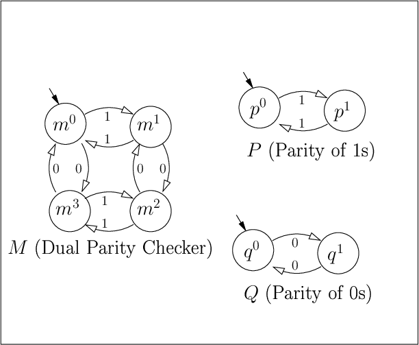
Consider the example shown in Fig. 8. Given the set of primaries $\{A,B,C\}$ shown in Fig. 1, we want to determine if $G$ can correct one crash fault among $\{A,B,C\}$ . Since $G$ is outside the closed partition set of $R$ , we first construct $B$ , which is the ${RCP}$ of $G$ and $R$ . Since $B$ is greater than both $R$ and $G$ , we can determine how its states are mapped to the states of $R$ and $G$ (similar to Fig. 2). For example, $b^{0}$ and $b^{8}$ are mapped to $r^{0}$ in $R$ , while $b^{0}$ and $b^{9}$ are mapped to $g^{0}$ in $G$ . Using this information, we can determine the mapping between the states of $R$ and $G$ . For example, since $b^{0}$ and $b^{9}$ are mapped to $r^{0}$ and $r^{2}$ respectively, $g^{0}=\{r^{0},r^{2}\}$ . Extending this idea, we get:

g^{1}=\{r^{1},r^{3}\};g^{2}=\{r^{6},r^{7}\};g^{3}=\{r^{4},r^{5}\};g^{4}=\{r^{0},r^{2}\}

In Fig. 3 $(ii)$ , the weakest edges of $G(\{A,B,C\})$ are $(r^{0},r^{1})$ and $(r^{2},r^{3})$ (the other weakest edges not shown). Since $G$ separates all these edges, it can correct one crash fault among the machines in $\{A,B,C\}$ . However, note that, the machines in $\{A,B,C\}$ cannot correct a fault in $G$ . For example, if $G$ crashes and $R$ is in state $r^{0}$ , we cannot determine if $G$ was in state $g^{0}$ or $g^{4}$ . This is clearly different from the case of the fusion machines presented in this paper, where faults could be corrected among both primaries and backups.

9 Related Work

Our work in [5] introduces the concept of the fusion of DFSMs, and presents an algorithm to generate a backup to correct one crash fault among a given set of machines. This paper is based on our work in [22, 4]. The work presented in [11, 2, 10] explores fault tolerance in distributed systems with programs hosting large data structures. The key idea there is to use erasure/error correcting codes [7] to reduce the space overhead of replication. Even in this paper, we exploit the similarity between fault tolerance in DFSMs and fault tolerance in a block of bits using erasure codes in section 3.3. However, there is one important difference between erasure codes involving bits and the DFSM problem. In erasure codes, the value of the redundant bits depend on the data bits. In the case of DFSMs, it is not feasible to transmit the state of all the machines after each event transition to calculate the state of the backup machines. Further, recovery in such an approach is costly due to the cost of decoding. In our solution, the backup machines act on the same inputs as the original machines and independently transition to suitable states. Extensive work has been done [16, 15] on the minimization of completely specified DFSMs, but the minimized machines are equivalent to the original machines. In our approach, we reduce the ${RCP}$ to generate efficient backup machines that are lesser than the ${RCP}$ . Finally, since we assume a trusted recovery agent, the work on consensus in the presence of Byzantine faults [18, 23], does not apply to our paper.

10 Conclusion

We present a fusion-based solution to correct $f$ crash or $\lfloor f/2\rfloor$ Byzantine faults among $n$ DFSMs using just $f$ backups as compared to the traditional approach of replication that requires $nf$ backups. In table 2, we summarize our results and compare the various parameters for replication and fusion. In this paper, we present a framework to understand fault tolerance in machines and provide an algorithm that generates backups that are optimized for states as well as events. Further, we present algorithms for detection and the correction of faults with minimal overhead over replication.

Our evaluation of fusion over standard benchmarks shows that efficient backups exist for many examples. To illustrate the practical use of fusion, we describe a fusion-based design of a distributed application in the MapReduce framework. While the current replication-based solution may require 1.8 million map tasks, a fusion-based solution requires just 1.4 million map tasks with minimal overhead in terms of time as compared to replication. This can result in considerable savings in space and other computational resources such as power.

In the future, we wish to implement the design presented in section 6 using the Hadoop framework [29] and compare the end-to-end performance of replication and our fusion-based solution. In particular we wish to focus on the space incurred by both solutions, the time and computation power taken for a set of tasks to complete with and without faults. Further, we wish to explore the existence of efficient backups if we allow information exchange among the primaries. Finally, we wish to design efficient algorithms to generate backups both inside and outside the closed partition set of the ${RCP}$ .

References

[1] Alexandr Andoni and Piotr Indyk. Near-optimal hashing algorithms for approximate nearest neighbor in high dimensions. Commun. ACM, 51(1):117–122, 2008.
[2] Bharath Balasubramanian and Vijay K. Garg. Fused data structures for handling multiple faults in distributed systems. In Proceedings of the 2011 31st International Conference on Distributed Computing Systems, ICDCS ’11, pages 677–688, Washington, DC, USA, 2011. IEEE Computer Society.
[3] Bharath Balasubramanian and Vijay K. Garg. Fused fsm design tool (implemented in java 1.6). In Parallel and Distributed Systems Laboratory, http://maple.ece.utexas.edu, 2011.
[4] Bharath Balasubramanian and Vijay K. Garg. Fused state machines for fault tolerance in distributed systems. In Principles of Distributed Systems - 15th International Conference, OPODIS 2011, Toulouse, France, December 13-16, 2011. Proceedings, volume 7109 of Lecture Notes in Computer Science, pages 266–282. Springer, 2011.
[5] Bharath Balasubramanian, Vinit Ogale, and Vijay K. Garg. Fault tolerance in finite state machines using fusion. In Proceedings of International Conference on Distributed Computing and Networking (ICDCN) 2008, Kolkata, volume 4904 of Lecture Notes in Computer Science, pages 124–134. Springer, 2008.
[6] Magdalena Balazinska, Hari Balakrishnan, Samuel Madden, and Mike Stonebraker. Fault-Tolerance in the Borealis Distributed Stream Processing System. In ACM SIGMOD Conf., Baltimore, MD, June 2005.
[7] E. R. Berlekamp. Algebraic Coding Theory. McGraw-Hill, New York, 1968.
[8] Jeffrey Dean and Sanjay Ghemawat. Mapreduce: simplified data processing on large clusters. Commun. ACM, 51:107–113, January 2008.
[9] Xavier Défago, André Schiper, and Péter Urbán. Total order broadcast and multicast algorithms: Taxonomy and survey. ACM Comput. Surv., 36(4):372–421, December 2004.
[10] Vijay K. Garg. Implementing fault-tolerant services using state machines: beyond replication. In Proceedings of the 24th international conference on Distributed computing, DISC’10, pages 450–464, Berlin, Heidelberg, 2010. Springer-Verlag.
[11] Vijay K. Garg and Vinit Ogale. Fusible data structures for fault tolerance. In ICDCS 2007: Proceedings of the 27th International Conference on Distributed Computing Systems, June 2007.
[12] Aristides Gionis, Piotr Indyk, and Rajeev Motwani. Similarity search in high dimensions via hashing. In VLDB ’99: Proceedings of the 25th International Conference on Very Large Data Bases, pages 518–529, San Francisco, CA, USA, 1999. Morgan Kaufmann Publishers Inc.
[13] Richard Hamming. Error-detecting and error-correcting codes. In Bell System Technical Journal, volume 29(2), pages 147–160, 1950.
[14] J. Hartmanis and R. E. Stearns. Algebraic structure theory of sequential machines (Prentice-Hall international series in applied mathematics). Prentice-Hall, Inc., Upper Saddle River, NJ, USA, 1966.
[15] John E. Hopcroft. An n log n algorithm for minimizing states in a finite automaton. Technical report, Stanford, CA, USA, 1971.
[16] David A. Huffman. The synthesis of sequential switching circuits. Technical report, Massachusetts, USA, 1954.
[17] Leslie Lamport. The implementation of reliable distributed multiprocess systems. Computer networks, 2:95–114, 1978.
[18] Leslie Lamport, Robert Shostak, and Marshall Pease. The Byzantine generals problem. ACM Transactions on Programming Languages and Systems, 4:382–401, 1982.
[19] David Lee and Mihalis Yannakakis. Closed partition lattice and machine decomposition. IEEE Trans. Comput., 51(2):216–228, 2002.
[20] P. M. Melliar-Smith, L. E. Moser, and V. Agrawala. Broadcast protocols for distributed systems. IEEE Trans. Parallel Distrib. Syst., 1(1):17–25, January 1990.
[21] Alan Mishchenko, Satrajit Chatterjee, and Robert Brayton. Dag-aware aig rewriting: A fresh look at combinational logic synthesis. In In DAC ’06: Proceedings of the 43rd annual conference on Design automation, pages 532–536. ACM Press, 2006.
[22] Vinit Ogale, Bharath Balasubramanian, and Vijay K. Garg. A fusion-based approach for tolerating faults in finite state machines. In Proceedings of the 2009 IEEE International Symposium on Parallel & Distributed Processing, IPDPS ’09, pages 1–11, Washington, DC, USA, 2009. IEEE Computer Society.
[23] M. Pease and L. Lamport. Reaching agreement in the presence of faults. Journal of the ACM, 27:228–234, 1980.
[24] Wesley W. Peterson and E. J. Weldon. Error-Correcting Codes - Revised, 2nd Edition. The MIT Press, 2 edition, March 1972.
[25] Fred B. Schneider. Byzantine generals in action: implementing fail-stop processors. ACM Trans. Comput. Syst., 2(2):145–154, 1984.
[26] Fred B. Schneider. Implementing fault-tolerant services using the state machine approach: A tutorial. ACM Computing Surveys, 22(4):299–319, 1990.
[27] Mehul A. Shah, Joseph M. Hellerstein, and Eric Brewer. Highly available, fault-tolerant, parallel dataflows. In Proceedings of the 2004 ACM SIGMOD International Conference on Management of Data, SIGMOD ’04, pages 827–838, New York, NY, USA, 2004. ACM.
[28] Fathi Tenzakhti, Khaled Day, and M. Ould-Khaoua. Replication algorithms for the world-wide web. J. Syst. Archit., 50(10):591–605, 2004.
[29] Tom White. Hadoop: The Definitive Guide. O’Reilly Media, Inc., 1st edition, 2009.
[30] Saeyang Yang. Logic synthesis and optimization benchmarks user guide version 3.0, 1991.
[31] Hiroshi Youra, Tomoo Inoue, Toshimitsu Masuzawa, and Hideo Fujiwara. On the synthesis of synchronizable finite state machines with partial scan. Systems and Computers in Japan, 29(1):53–62, 1998.

Appendix A Event-Based Decomposition of Machines

In this section, we ask a question that is fundamental to the understanding of DFSMs, independent of fault-tolerance: Given a machine $M$ , can it be replaced by two or more machines executing in parallel, each containing fewer events than $M$ ? In other words, given the state of these fewer-event machines, can we uniquely determine the state of $M$ ? In Fig. 11, the 2-event machine $M$ (it contains events 0 and 1 in its event set), checks for the parity of 0s and 1s. $M$ can be replaced by two 1-event machines $P$ and $Q$ , that check for the parity of just 1s or 0s respectively. Given the state of $P$ and $Q$ , we can determine the state of $M$ . In this section, we explore the problem of replacing a given machine $M$ with two or more machines, each containing fewer events than $M$ . We present an algorithm to generate such event-reduced machines with time complexity polynomial in the size of $M$ . This is important for applications with limits on the number of events each individual process running a DFSM can service. We first define the notion of event-based decomposition.

Definition 5

A (k,e)-event decomposition of a machine $M$ $(X_{M}$ , $\alpha_{M}$ , $\Sigma_{M}$ , $m^{0})$ is a set of $k$ machines $\mathcal{E}$ , each less than $M$ , such that $d_{min}(M,\mathcal{E})>0$ and $\forall P(X_{P},\alpha_{P},\Sigma_{P},p^{0})\in\mathcal{E}$ , $|\Sigma_{P}|\leq|\Sigma_{M}|-e$ .

As $d_{min}(M,\mathcal{E})>0$ , given the state of the machines in $\mathcal{E}$ , the state of $M$ can be determined. So, the machines in $\mathcal{E}$ , each containing at most $|\Sigma_{M}|-e$ events, can effectively replace $M$ . In Fig. 12, we present the eventDecompose algorithm that takes as input, machine $M$ , parameter $e$ , and returns a ( $k$ , $e$ )-event decomposition of $M$ (if it exists) for some $k\leq|X_{M}|^{2}$ .

In each iteration, Loop 1 generates machines that contain at least one event less than the machines of the previous iteration. So, starting with $M$ in the first iteration, at the end of $e$ iterations, $\mathcal{M}$ contains the set of largest machines less than $M$ , each containing at most $|\Sigma_{M}|-e$ events.

Loop 2, iterates through each machine $P$ generated in the previous iteration, and uses the reduceEvent algorithm (same as the algorithm presented in Fig. 4) to generate the set of largest machines less than $P$ containing at least one event less than $\Sigma_{P}$ . To generate a machine less than $P$ , that does not contain an event $\sigma$ in its event set, the reduceEvent algorithm combines the states such that they loop onto themselves on $\sigma$ . The algorithm then constructs the largest machine that contains these states in the combined form. This machine, in effect, ignores $\sigma$ . This procedure is repeated for all events in $\Sigma_{P}$ and the largest incomparable machines among them are returned. Loop 3 constructs an event-decomposition $\mathcal{E}$ of $M$ , by iteratively adding at least one machine from $\mathcal{M}$ to separate each pair of states in $M$ , thereby ensuring that $d_{min}(\mathcal{E})>0$ . Since each machine added to $\mathcal{E}$ can separate more than one pair of states, an efficient way to implement Loop 3 is to check for the pairs that still need to be separated in each iteration and add machines till no pair remains.

Let the 4-event machine $M$ shown in Fig. 12 be the input to the eventDecompose algorithm with $e=1$ . In the first and only iteration of Loop 1, $P=M$ and the reduceEvent algorithm generates the set of largest 3-event machines less than $M$ , by successively eliminating each event. To eliminate event 0, since $m^{0}$ transitions to $m^{3}$ on event $0$ , these two states are combined. This is repeated for all states and the largest machine containing all the combined states self looping on event 0 is $M_{1}$ . Similarly, the largest machines not acting on events 3,1 and 2 are $M_{2}$ , $M_{3}$ and $M_{\bot}$ respectively. The reduceEvent algorithm returns $M_{1}$ and $M_{2}$ as the only largest incomparable machines in this set. The eventDecompose algorithm returns $\mathcal{E}=\{M_{1}$ , $M_{2}\}$ , since each pair of states in $M$ are separated by $M_{1}$ or $M_{2}$ . Hence, the 4-event $M$ can be replaced by the 3-event $M_{1}$ and $M_{2}$ , i.e., $\mathcal{E}=\{M_{1},M_{2}\}$ is a (2,1)-event decomposition of $M$ .

Theorem A.1

Given machine $M$ $(X_{M},\alpha_{M},\Sigma_{M},m^{0})$ , the eventDecompose algorithm generates a ( $k$ , $e$ )-event decomposition of $M$ (if it exists) for some $k\leq|X_{M}|^{2}$ .

Proof

The reduceEvent algorithm exhaustively generates the largest incomparable machines that ignore at least one event in $\Sigma_{M}$ . After $e$ such reduction in events, Loop 3 selects one machine (if it exists) among $\mathcal{M}$ to separate each pair of states in $X_{M}$ . This ensures that at the end of Loop 3, either $d_{min}(\mathcal{E})>0$ or the algorithm has returned $\{\}$ (no ( $k$ , $e$ )-event decomposition exists). Since there are at most $|X_{M}|^{2}$ pairs of states in $X_{M}$ , there are at most $|X_{M}|^{2}$ iterations of Loop 3, in which we pick one machine per iteration. Hence, $k\leq|X_{M}|^{2}$ .

The reduceEvent algorithm visits each state of machine $M$ to create blocks of states which loop to the same block on event $\sigma\in\Sigma_{M}$ . This has time complexity $O(|X_{M}|)$ per event. The cost of generating the largest closed partition corresponding to this block is $O(|X_{M}||\Sigma_{M}|)$ per event. Since we need to do this for all events in $\Sigma_{M}$ , the time complexity to reduce at least one event is $O(|X_{M}||\Sigma_{M}|^{2})$ . In the eventDecompose algorithm, the first iteration generates at most $|\Sigma_{M}|$ machines, the second iteration at most $|\Sigma_{M}|^{2}$ machines and the $e^{th}$ iteration will contain $O(|\Sigma_{M}|^{e})$ machines. The rest of the analysis is similar to the one presented in section 4.2 and the time complexity of the reduceEvent algorithm is $O(|X_{M}||\Sigma_{M}|^{e+1})$ .

To generate the ( $k$ , $e$ )-event decomposition from the set of machines in $\mathcal{M}$ , we find a machine in $\mathcal{M}$ to separate each pair of states in $X_{M}$ . Since there are $O(|X_{M}|^{2})$ such pairs, the number of iterations of Loop 3 is $O(|X_{M}|^{2})$ . In each iteration of Loop 3, we find a machine among the $O(|\Sigma_{M}|^{e})$ machines of $\mathcal{M}$ that separates a pair $m_{i},m_{j}\in X_{M}$ . To check if a machine separates a pair of states just takes $O(|X_{M}|)$ time. Hence the time complexity of Loop 3 is $O(|X_{M}|^{3}|\Sigma_{M}|^{e})$ . So, the overall time complexity of the eventDecompose algorithm is the sum of the time complexities of Loop 1 and 3, which is $O(|X_{M}||\Sigma_{M}|^{e+1}+|X_{M}|^{3}|\Sigma|^{e})$ .

Appendix B Incremental Approach to Generate Fusions

incFusion Input: Primaries $\mathcal{P}=\{P_{1},P_{2},\ldots P_{n}\}$ , faults $f$ ,
state-reduction parameter $\bigtriangleup s$ , event-reduction parameter $\bigtriangleup e$ ;
Output: ( $f$ , $f$ )-fusion of $\mathcal{P}$ ;
$\mathcal{F}\leftarrow\{P_{1}\}$ ;
for ( $i=2$ to $n$ )
$\mathcal{N}\leftarrow\{P_{i}\}\cup{RCP}(\mathcal{F})$ ;
$\mathcal{F}\leftarrow\emph{genFusion}(\mathcal{N},f,\bigtriangleup s,\bigtriangleup e)$ ;
return $\mathcal{F}$ ;

Figure 13: Incremental fusion algorithm.

In Fig. 13, we present an incremental approach to generate the fusions, referred to as the incFusion algorithm, in which we may never have to reduce the ${RCP}$ of all the primaries. In each iteration, we generate the fusion corresponding to a new primary and the ${RCP}$ of the (possibly small) fusions generated for the set of primaries in the previous iteration.

In Fig. 14, rather than generate a fusion by reducing the 8-state ${RCP}$ of $\{A,B,C\}$ , we can reduce the 4-state ${RCP}$ of $\{A,B\}$ to generate fusion $F^{\prime}$ and then reduce the 4-state ${RCP}$ of $\{C,F^{\prime}\}$ to generate fusion $F$ . In the following paragraph, we present the proof of correctness for the incremental approach and show that it has time complexity $O(\rho^{n})$ times better than that of the genFusion algorithm, where $\rho$ is the average state reduction achieved by fusion.

Theorem B.1

Given a set of $n$ machines $\mathcal{P}$ , the incFusion algorithm generates an ( $f$ , $f$ )-fusion of $\mathcal{P}$ .

Proof

We prove the theorem using induction on the variable $i$ in the algorithm. For the base case, i.e., $i=2$ , $\mathcal{N}=\{P_{1},P_{2}\}$ (since $RCP(\{P_{1}\})=P_{1}$ ). Let the ( $f$ , $f$ )-fusion generated by the genFusion algorithm for $\mathcal{N}=\{P_{1},P_{2}\}$ be denoted $\mathcal{F}^{1}$ . For $i=3$ , let the ( $f$ , $f$ )-fusion generated for $\mathcal{N}=\{P_{3},{RCP}(\mathcal{F}^{1})\}$ be denoted $\mathcal{F}^{2}$ . We show that $\mathcal{F}^{2}$ is an ( $f$ , $f$ )-fusion of $\{P_{1},P_{2},P_{3}\}$ . Assume $f$ crash faults among $\{P_{1}P_{2},P_{3}\}\cup\mathcal{F}^{2}$ . Clearly, less than or equal to $f$ machines in $\{P_{3}\}\cup\mathcal{F}^{2}$ have crashed. Since $\mathcal{F}^{2}$ is an ( $f$ , $f$ )-fusion of $\{P_{3},{RCP}(\mathcal{F}^{1})\}$ , we can generate the state of all the machines in ${RCP}(\mathcal{F}^{1})$ and the state of the crashed machines among $\{P_{3}\}\cup\mathcal{F}^{2}$ . Similarly, less than or equal to $f$ machines have crashed among $\{P_{1},P_{2}\}$ . Hence, using the state of the available machines among $\{P_{1},P_{2}\}$ and the states of all the machines in $\mathcal{F}^{1}$ we can generate the state of the crashed machines among $\{P_{1},P_{2}\}$ .

Induction Hypothesis: Assume that the set of machines $\mathcal{F}^{i}$ , generated in iteration $i$ , is an ( $f$ , $f$ )-fusion of $\{P_{1}\ldots P_{i+1}\}$ . Let the ( $f$ , $f$ )-fusion of $\{P_{i+2},{RCP}(\mathcal{F}^{i})\}$ generated in iteration $i+1$ be denoted $\mathcal{F}^{i+1}$ . To prove: $\mathcal{F}^{i+1}$ is an ( $f$ , $f$ )-fusion of $\{P_{1}\ldots P_{i+2}\}$ . The proof is similar to that for the base case. Using the state of the available machines in $\{P_{i+2}\}\cup\mathcal{F}^{i+1}$ , we can generate the state of all the machines in $\mathcal{F}^{i}$ and $\{P_{i+2}\}\cup\mathcal{F}^{i+1}$ . Subsequently, we can generate the state of the crashed machines in $\{P_{1}\ldots P_{i+1}\}$ .

From observation 1, the genfusion algorithm has time complexity,
$O(fN^{4}|\Sigma|+fN^{5})$ (assuming $\bigtriangleup s=0$ and $\bigtriangleup e=0$ for simplicity). Hence, if the size of $\mathcal{N}$ in the $i^{th}$ iteration of the incFusion algorithm is denoted by $N_{i}$ , then the time complexity of the incFusion algorithm, $T_{inc}$ is given by the expression $\Sigma_{i=2}^{i=n}O(fN_{i}^{4}|\Sigma|+fN_{i}^{5})$ .

Let the number of states in each primary be $s$ . For $i=2$ , the primaries are $\{P_{1},P_{2}\}$ and $N_{1}=O(s^{2})$ . For $i=3$ , the primaries are { ${RCP}(\mathcal{F}^{1}),P_{3}\}$ . Note that ${RCP}({\mathcal{F}^{1})}$ is also a fusion machine. Since we assume an average reduction of $\rho$ (size of ${RCP}$ of primaries/average size of each fusion), the number of states in ${RCP}(\mathcal{F}^{1})$ is $O(s^{2}/\rho)$ . So , $N_{2}=O(s^{3}/\rho)$ . Similarly, $N_{3}=O(s^{4}/\rho^{2})$ and $N_{i}=O(s^{i+1}/\rho^{i-1})$ . So,

T_{inc}=O(|\Sigma|f\Sigma_{i=2}^{i=n}s^{4i+4}/\rho^{4i-4}+f\Sigma_{i=2}^{i=n}s^{5i+5}/\rho^{5i-5})

=O(|\Sigma|fs^{4}\rho^{4}\Sigma_{i=2}^{i=n}(s/\rho)^{4i}+fs^{5}\rho^{5}\Sigma_{i=2}^{i=n}(s/\rho)^{5i})

This is the sum of a geometric progression and hence,

T_{inc}=O(|\Sigma|fs^{4}\rho^{4}(s/\rho)^{4n}+fs^{5}\rho^{5}(s/\rho)^{5n})

Assuming $\rho$ and $s$ are constants, $T_{inc}=O(f|\Sigma|s^{n}/\rho^{n}+fs^{n}/\rho^{n})$ . Note that, the time complexity of the genFusion algorithm in Fig. 4 is $O(f|\Sigma|s^{n}+fs^{n})$ . Hence, the incFusion algorithm achieves $O(\rho^{n})$ savings in time complexity over the $\emph{genFusion}$ algorithm.

Fault Tolerance in Distributed Systems using Fused State Machines

Abstract

Keywords:

1 Introduction

Framework for Fault Tolerance in DFSMs

Algorithm to Generate Fused Backup Machines

Detection and Correction of Faults

Fusion-based Grep in the MapReduce Framework

Fusion-based Design Tool and Experimental Evaluation

2 Model

3 Framework for Fault Tolerance in DFSMs

3.1 DFSMs and their Reachable Cross Product

3.2 Order Among Machines and their Closed Partition Lattice

3.3 Fault Graphs and Hamming Distances

Definition 1

Definition 2

Theorem 3.1

Proof

Theorem 3.2

Proof

3.4 Theory of (ff, mm)-fusion

Definition 3

Theorem 3.3

Proof

Theorem 3.4

Proof

Definition 4

Theorem 3.5

Proof

4 Algorithm to Generate Fused Backup Machines

4.1 Properties of the genFusion Algorithm

Lemma 1

Proof

Lemma 2

Proof

Lemma 3

Proof

Theorem 4.1

Proof

4.2 Time Complexity of the genFusion Algorithm

Observation 1

5 Detection and Correction of Faults

5.1 Detection of Byzantine Faults

Theorem 5.1

Proof

5.2 Correction of Faults

5.2.1 Crash Correction

Theorem 5.2

Proof

5.2.2 Byzantine Correction

Theorem 5.3

Proof

6 Practical use of Fusion in the MapReduce Framework

6.1 Existing Replication-based Solution

6.2 Hybrid Fusion-based Solution

7 Experimental Evaluation

8 Discussion: Backups Outside the Closed Partition Set

9 Related Work

10 Conclusion

References

Appendix A Event-Based Decomposition of Machines

Definition 5

Theorem A.1

Proof

Appendix B Incremental Approach to Generate Fusions

Theorem B.1

Proof

3.4 Theory of ( $f$ , $m$ )-fusion