IMPULSE RADIO ULTRA-WIDEBAND COMMUNICATION OVER FREE-SPACE OPTICAL LINKS
by
Kemal Davaslıoğlu
B.S. Electrical and Electronics Engineering, Bilkent University, 2008
Submitted to the Institute for Graduate Studies in
Science and Engineering in partial fulfillment of
the requirements for the degree of
Master of Science
Graduate Program in Electrical and Electronics Engineering
Boğaziçi University
2026
ABSTRACT
A composite impulse radio ultra-wideband (IR-UWB) communication system is presented. The proposed system model aims to transmit UWB pulses over several kilometers through free-space optical (FSO) links and depending on the link design, the electrical estimates of the FSO system can be directly used or distributed to end-user through radio-frequency (RF) links over short ranges. However, inhomogeneities on the FSO transmission path cause random fluctuations in the received signal intensity and these effects induced by atmospheric turbulence closely effect the system performance. Several distinct probability distributions based on experimental measurements are used to characterize FSO channels and using these probabilistic models, detection error probability analysis of the proposed system for different link designs are carried out under weak, moderate and strong turbulence conditions. The results of the analysis show that depending on the atmospheric conditions, system performance of the composite link can have high error floors due to the false estimates of FSO link. The system performance can be improved by employing error control coding techniques. One simple solution employing a convolutional encoder and Viterbi decoder pair is also analyzed in this thesis. Another important system parameter that is the average channel capacity of the FSO system is analyzed under weak and moderate turbulence conditions. Theoretical derivations that are verified via simulation results indicate a reliable high data rate communication system that is effective in long distances.
IMPULSE RADIO ULTRA-WIDEBAND COMMUNICATION OVER FREE-SPACE OPTICAL LINKS
APPROVED BY:
| Assist. Prof. Mutlu Koca | . |
| (Thesis Supervisor) | |
| Prof. Hakan Deliç | . |
| Prof. Naci İnci | . |
DATE OF APPROVAL: 29.07.2010
ACKNOWLEDGEMENTS
First of all, I would like to thank Assist. Prof. Mutlu Koca for his help, encouragement and support throughout my study in Boǧaziçi University. Since the first day I stepped in to this university, he was there with me. His help has enabled me to understand and develop a strong intuition on telecommunications and his way of looking at things has always impressed me. His critical suggestions have definitely improved my work and this thesis could not be accomplished without his guidance.
I also wish to thank to the committee members Prof. Hakan Deliç and Prof. Naci İnci for their important suggestions and valuable comments that have shaped the final version of my thesis.
I am also grateful to Assist. Prof. Ali Emre Pusane and Assoc. Prof. M. Kıvanç Mıhçak for sharing their experience and valuable ideas on both engineering and career which helped me broaden my approach and I owe them a lot.
My friends and colleagues were always with me whenever I needed to chat and with their friendship I was able to clear my mind and focus clearly. Especially, Erman Çağıral, Yakup Kılıç, Berksan Şerbetçi, Oğuzhan Kondakçı, Temuçin Som, N. Caner Göv, Hasan Sicim, Kamil Şenel and Deniz Seviş are just to name a few. Also, I should give a special thanks to Duygu Eruçman who has always supported me with her presence and delicious food.
Last but not least, I am deeply grateful to my parents Ali and Bilge Davaslıoğlu and my grandparents Kemal and Gülseren Özmen for their eternal love and support. I will always have my utmost and deepest gratitude toward them.
This thesis is supported by the Scientific and Technological Research Council of Turkey (TUBITAK) under the grant number 105E077.
ÖZET
OPTİK SERBEST-UZAY KANALLARINDA DARBE-RADYO ULTRA-GENİŞBANT HABERLEŞİMİ
Bu çalışmada karma darbe-radyo ultra-genişbant haberleşme sistemi önerilmiştir. Önerilen sistem modeli ultra-genişbant sinyalleri optik serbest uzay (OSU) üzerinden uzun mesafelerde taşıması amaçlanmıştır ve sistem tasarımına bağlı olarak elektriksel OSU kestirimleri direkt olarak kullanılabilir veya son kullanıcıya radyo frekansı (RF) üzerinden kısa mesafelerde dağıtım yapabilir. Ancak, OSU gönderim kanallarındaki türdeşsizlikler alınan sinyalin yoğunluğunda dalgalanmalara neden olur ve atmosferdeki türbülans kaynaklı bu etkiler sistem performansını yakından etkilemektedir. OSU kanalları tanımlamak için deneysel ölçümlerden çıkarılan belirli istatistiksel dağılımlar mevcuttur ve bu modelleri kullanarak önerilen sistemin hata olasılık analizi zayıf, orta ve sert türbülans bölgelerinde incelenmiştir. Yapılan teorik analiz sonuçlarına göre atmosfer koşullarına bağlı olarak sistem performansında yanlış OSU kestirimlerinin getirdiği yüksek hata tabanları gözlemlenmiştir. Sistem performansının iyileştirilmesi için hata kontrol kodlaması önerilmiştir. Örnek olarak, OSU sisteminde gönderici tarafında evrişimli kodyalıcı ve alıcı tarafında Viterbi kodçözücüsü kullanıldığı durum incelenmiş ve bu durumun hata olasılık analizi yapılmıştır. Önemli bir başka sistem parametresi, ortalama kanal kapasitesi OSU kanallar için zayıf ve orta türbülans koşullarında incelemiştir. Simulasyon sonuçları ile doğrulanan teorik çıkarımlar, önerilen sistemin uzun mesafelerde güvenilir bir şekilde yüksek veri hızlarına çıkabileceğini göstermiştir.
TABLE OF CONTENTS
LIST OF FIGURES
LIST OF TABLES
LIST OF SYMBOLS/ABBREVIATIONS
| Path loss at a reference distance of 1 meters | |
| Wavenumber spectrum structure parameter | |
| D | The link distance |
| Diameter of the receiver aperture | |
| Correlation length of the atmospheric turbulence | |
| Expectation operation | |
| Energy of the received pulse | |
| Energy of the transmitted pulse | |
| Fourier transformation operation | |
| Center frequency of the transmitted message | |
| Higher frequency of the -10 dB emission point | |
| Lower frequency of the -10 dB emission point | |
| Average total multi-path gain | |
| Meijer’s G-function | |
| The reference power gain evaluated at 1 meters | |
| Mean of the random variable | |
| FSO channel | |
| RF channel | |
| Light intensity | |
| Mutual information between random variables denoted by and | |
| Mean of light intensity | |
| order modified Bessel function of second kind | |
| Wavenumber | |
| L | Link distance |
| Outer scale of turbulence | |
| Inner scale of turbulence | |
| m | Meters |
| Nanometers | |
| Refractive index | |
| Average refractive index | |
| Fluctuation component induced by spatial variations of both pressure and temperature | |
| Path loss at a reference distance of 1 meters | |
| Bernoulli random variable | |
| Arrival time of the cluster | |
| Root mean square of the wind speed | |
| Random variable denoting log-amplitude fluctuations of the atmospheric turbulence channel | |
| FSO-UWB TH-PPM pulse | |
| RF-UWB TH-PPM pulse | |
| Effective height of the turbulent atmosphere | |
| Random variable denoting small scale scatters | |
| The channel coefficient of the cluster multipath | |
| Random variable denoting large scale scatters | |
| The log-normal distributed channel coefficient of cluster path | |
| Dirac-delta function | |
| Electro-optical conversion coefficient | |
| Power decay factor for clusters | |
| Gamma function | |
| Autocorrelation function of | |
| Log-normal fading random variable | |
| Gaussian random variable | |
| Poisson arrival rate of clusters | |
| Poisson arrival rate of multipaths within clusters | |
| Wavelength | |
| Mean of the random variable | |
| Normalization factor of the total received power | |
| Wavenumber spectrum | |
| Variance of the channel amplitude gain | |
| Variance of log-amplitude fluctuations in terms of scintillation index | |
| Scintillation index | |
| Variance of log-amplitude fluctuations | |
| Variance of the fluctuations of the channel coefficient for clusters | |
| Variance of the fluctuations of the channel coefficients for rays within clusters | |
| Rytov variance for plane waves | |
| Rytov variance for spherical waves | |
| Channel coefficient of fluctuations on each cluster | |
| The arrival time of the paths (rays) of the cluster | |
| Channel coefficient of fluctuations on each contribution | |
| AWGN | Additive white Gaussian noise |
| BER | Bit error rate |
| BPSK | Binary phase shift keying |
| CD | Compact disc |
| CEPT | European Conference of Postal and Telecommunications |
| CLT | Central limit theorem |
| CM1 | Channel model 1 |
| DVD | Digital versatile disc |
| DEP | Detection error probability |
| ECC | Electronic Communications Committee |
| EDFA | Erbium-doped fiber amplifier |
| EIRP | The equivalent isotropic radiated power |
| FCC | Federal Communications Commission in the United States |
| FPLD | Gain-switched Fabry-Perot laser diode (FPLD) |
| FSO | Free-Space Optics |
| GPS | Global Positioning System |
| IEEE | Institute of Electrical and Electronics Engineers |
| IR | Impulse Radio |
| ITU | International Telecommunications Union |
| LOS | Line-of-sight |
| ML | Maximum-likelihood |
| MLSD | Maximum-likelihood sequence detection |
| NLOS | Non-line-of-sight |
| OOK | On-Off keying |
| PAN | Personal Area Network |
| Probability density function | |
| PPM | Pulse position modulation |
| RF | Radio frequency |
| RMS | Root mean square |
| SNR | Signal-to-noise ratio |
| S-V | Saleh Valenzuela |
| TF | Tunable Filter |
| TH | Time-hopping |
| UWB | Ultra-Wideband |
| WDM | Wavelength division multiplexing |
| WLAN | Wireless Local Area Networks |
| WPAN | Wireless Personal Area Networks |
Chapter 1 INTRODUCTION
Ultra-wideband (UWB) systems characterize those that employ very narrow pulses in time usually on the order of nanoseconds to convey information. Consequently, these pulses occupy very large bandwidths in frequency domain. Due to their characteristics, UWB systems have unique attractive features introducing new advances in several wireless communications fields such as radar, imaging, networking and positioning systems. These aforementioned fields benefit from several advantages offered by UWB systems such as enhanced ability to penetrate through obstacles such as concrete walls, ultra high precision ranging, possibility to transmit at very high data rates and support multi-user, relatively small size and less power consumption [1]. Until 2001, the use of UWB systems were limited solely to military applications and with the regulations introduced by the Federal Communications Commission (FCC) in the United States, these new features of UWB systems have gained its attraction in several areas [2]. The FCC in the United States has allocated a huge unlicensed frequency spectrum ranging from 3.1 GHz to 10.6 GHz for UWB systems. These pulses need occupy at least 500 MHz of bandwidth within the allowed spectrum or a fractional bandwidth of more than 20 percent where the fractional bandwidth defines the ratio of bandwidth over the center frequency . Since UWB systems do not employ any carrier to transmit the signals, the definition of center frequency needs to be clarified. The lower and higher frequencies of dB emission points on the power spectrum of the transmitted signal are denoted by and and their arithmetic mean determines the center frequency of the signal, . Also, the bandwidth of the signal is defined as the difference of these two frequencies, [1].
Although wireless propagation channels have been studied for more than 50 years and several mathematical models are introduced in literature to describe their propagation characteristics, the FCC in the United States have accepted the IEEE 802.15.3a channel model for the indoor and outdoor UWB channels with the contribution from Intel Corporation in 2002. This regulation for UWB systems are primarily developed for Wireless Personal Area Networks (WPAN) and to enable the coexistence of UWB systems with the current technologies, namely, the Bluetooth and the IEEE 802.11 wireless local are networks (WLAN), the FCC in the United States has defined the spectral mask that every UWB device needs to accompany which is presented in the next chapter.
Although UWB systems bring their unique advantages, they are limited to short distances, usually up to 10 meters, due to severe attenuation of these narrow pulses. To overcome this short range limitation in radio frequency (RF) links, free-space optical (FSO) systems have emerged as a cost efficient solution. Compared to RF systems, FSO links offer much larger bandwidth and capacity, less power consumption, more robust against eavesdropping and better protection against interference [3]. Although FSO systems are mainly used in inter-satellite and deep space communications, these systems have attracted considerable attention to solve the last-mile solution in the past decade [4].
Contrary to other emerging alternatives to RF links, theoretical background of FSO systems are known and they are very similar to the fiber-optical communication systems. In these systems, information can be conveyed in the intensity, frequency, phase or polarization of the signal. Among these attributes, intensity is typically used to carry information due to its simplicity and this type of modulation employing variations in intensity is called intensity modulation. Because of the complexities associated with phase or frequency of the received signal, these type of modulation are not preferred in most FSO systems [5].
Along with the power regulations concerning eye safety, FSO system performance are also limited by the atmospherical effects. The inhomogeneities in the atmosphere cause fluctuations in the amplitude and phase of the received signal over long distances and these effects severely degrade the performance of the system. Besides the inhomogeneities in the atmosphere, aerosol scatterers such as rain, snow and fog and building-sway as a result of wind loads, thermal expansion and weak earthquakes are the other factors degrading the system performance [5, 6]. For instance, under severe fog conditions, it has been reported that the signals attenuate on the order of hundreds of decibels per kilometer [7].
1.1 Research Overview and Contributions
This work addresses the short range coverage problem of UWB systems that operate in RF links. To overcome this bottleneck, an alternative technique is proposed and UWB signals are transmitted through FSO links over several kilometers in the last mile. In FSO systems, the impairments caused by the atmospheric turbulence closely effect the system performance on the transmission path and therefore, there has been extensive studies and models proposed to describe these conditions and these can be found in [8]-[13]. Recent studies using these models investigate the performance of FSO links under atmospheric turbulence effects such as those in [4, 5, 6, 14, 15]. In their pioneering work, Zhu and Kahn have applied maximum-likelihood sequence detection (MLSD) technique to mitigate the effects of atmospheric turbulence at the cost of increased complexity [5]. They have also included maximum-likelihood detection under the case when spatial diversity is available. In [6], the authors have analyzed the performance of FSO system for both correlated and independent channels under weak turbulence conditions. The performance analysis of a FSO system that use pulse position modulation scheme under weak turbulence conditions is presented in [14] and in their system model, the authors employ avalanche photodiode to receive the signals. In his study, Kiasaleh carries out the same analysis for the same type of photodetector but this time, the analysis includes the effects of moderate turbulence conditions [4]. Another recently published work in [15], the authors investigate the system performance under a more accurate statistical distribution to model the moderate weather conditions. Besides error analysis, the ergodic channel capacity of FSO links in the weak turbulence regime is derived in [16] and for the moderate regime, its closed-form expression is presented in [17]. Also, Hranilovic et. al derive outage capacity analysis of an FSO system considering the effects of pointing errors in [18] and Uysal et. al apply a relay system to their FSO system model in [19].
However, this work focuses solely on conveying UWB signals through FSO links over long distances and to this end, several system models are proposed. In the first system model, the generated optical UWB signals can be transmitted over FSO links over long distances and at the receiver the detected electrical outputs can be used right away or distributed to the end-user within the building using ethernet or fiber cables at very high-speeds. It should be emphasized again that FSO systems can achieve very high data speeds that are compatible with fiber optical and ethernet cables can support. As an extension of the first case, the second scenario considers the case that the UWB signals are again conveyed over FSO links in the last-mile but this time the electrical outputs are distributed to the end-users by the RF link in the last-step by employing a simple UWB transmitter and receiver pair. Third scenario uses error-control techniques in the FSO link to reduce the possible errors induced by the turbulence effects. Although under good weather conditions the system performance can achieve superior results, as the link visibility decreases or weather conditions gets worse, error-control coding is a necessity to endure the availability of the link and improve the quality of service of the system. For all three scenarios, corresponding system models are presented and their analytical results for the detection error probability under different turbulence conditions are analyzed. These theoretical results are verified via simulations that confirm the presented results. To sum up, the biggest contribution of this thesis is the complete error analysis of the aforementioned system designs that enable long distance transmission of UWB signals through FSO links. This contribution is valuable because UWB systems suffer from their short range limitations and the proposed models in this thesis would help to overcome this bottleneck.
1.2 Organization of the Thesis
Chapter 2 provides brief information about impulse-radio ultra-wideband systems. It presents several factors that are considered to model channel distributions in RF links and introduces the spectral mask proposed by several regulatory institutions in Europe and United States that enables the coexistence of these devices with the other equipments in the same frequency spectrum. In its first section, several sources of fading are discussed in detail and particular examples are given from daily life. In the next section, the accurate distribution to model the RF-UWB links are discussed. This accepted model is mainly based on Saleh-Valenzuela model with some modifications. Parameters definitions and suggested values of these parameters are also presented towards the end of the chapter. Chapter 3 focuses on wireless optical systems. It discusses several commonly used modulation techniques in these systems and introduces some conditions on the reception of the transmitted signal along with some important parameters that determine the link quality. Its first section explains the characteristics of FSO channel in detail and the last section of the chapter introduces the statistical models for different turbulence conditions. Chapter 4 discusses the proposed system model in this thesis. Along with the devices used in the system model, their mathematical interpretations are also given. Detection error probability analysis of the several possible scenarios carried out. For instance, closed form expression are derived for the scenario where the FSO link is used to convey the information over several kilometers and the RF link to deliver the signal to the end-user in the last-step and simulations are made to verify theoretical results. This chapter is concluded with the channel capacity analysis of the FSO links. Finally, the last chapter addresses several concluding remarks and suggestions for possible future work.
Chapter 2 IMPULSE-RADIO ULTRA-WIDEBAND SYSTEMS
In wired channels such as coaxial cables, wave propagation is predictable and usually stationary whereas in radio channels, the behavior of wave propagation extremely random in nature [20]. There are several sources that effect electromagnetic wave propagation in radio frequency (RF) channels such as absorption, diffraction, reflection and scattering which all gives rise to multiple paths. On the path between transmitter and receiver, the objects are highly likely to be absorb, diffract, reflect or scatter the energy of the waves causing the signals to travel by various amplitudes, phases and paths before it reaches to the receiver. The propagation of these waves (echoes of the original transmitted signal) are called multipath propagation and the phenomenon of amplitude and phase fluctuations in the received signal due to multipath propagation is called multipath fading [21]. Since each wave travels different lengths of paths, pulses arrive at the receiver at different times with different amplitudes and phases. Therefore, to describe the behavior of the channel in different environments, several channel models are proposed. These proposed models are mostly based results measured from experimental data.
Several multipath components arrive to the receiver and collectively determine the amplitude and phase of the received signal. The first statistical model which is still widely used is Rayleigh fading channel model and it applies to the conditions when the bandwidth of the signal is small and the delays of the individual multipath components do not interfere with each other in the received signal model. This signal model assumes that there are almost no significant scatterers nor dominant signal reflectors in the channel. The other widely accepted channel model is Ricean fading channel and it considers the case when the channel exhibits fixed scatters or signal reflectors in the channel [22].
Although these models are sufficient to characterize channels for narrow-band systems, more accurate description to capture the behavior of the multipath components is needed to characterize systems that occupy ultra-wide bandwidths. For this purpose, several studies have been made. In 2002, the IEEE has established a standardization group, IEEE 802.15.3a to a develop standard for UWB Personal Area Networks (PANs). They were to select the multiple access schemes, modulations and a commonly agreed channel model along with the other necessity of the standard. To this end, IEEE 802.15.3a Task Group had been formed and established a standard channel model to be used for the evaluation of PAN physical layer proposals. The Federal Communications Commission (FCC) in the United States has also decided on the data rates for the standard model under the regulated power levels below dBm in Part 15 rules to coexist with the already available services such as Global Positioning System (GPS) and the IEEE 802.11 wireless local are networks (WLANs). IEEE 802.15.3a standard model aims to transmit at data rates up to 100 Mbs at 10 meters, 200 Mbs at 4 meters and higher data rates at smaller distances [23].
The allocated spectrum to transmit these signals ranges from 3.1 GHz to 10.6 GHz and this ultra-wide bandwidth allows for several bandwidth-demanding low power applications in wireless communications such as short-range high-speed Internet access, vehicular radar and sensors, asset and personnel tracking, imaging through steel and walls, surveillance and medical monitoring applications [1]. It should be emphasized that UWB signals are on the order of nanoseconds scale so that their power spectral density occupies such bandwidths without the need for any carrier. Depending on the pulse width, these signals can be designed to occupy all the 7.5 GHz spectrum in a single-band or several multi-band UWB signals can be created such that each occupies at minimum bandwidth of 500 MHz. The former is called as impulse-radio ultra-wideband (IR-UWB) signalling and the latter is referred to as multi-band UWB signalling where each has its own consequences and this work focuses solely on IR-UWB signalling.
On the other hand, UWB technology faces several challenges such as bit error rate, capacity and throughput limitations due to low-power regulations, network flexibility, immunity to synchronization and many more. Along with these challenges, the FCC has released a spectral mask that limits the equivalent isotropic radiated power (EIRP) spectrum density of the UWB pulses to fully coexist with the other aforementioned technologies and this is shown in Fig. 2.1 and Tables 2.1 and 2.2 along with the regulations introduced by European Conference of Postal and Telecommunications (CEPT) and International Telecommunications Union (ITU). Pulse shaping filters are commonly used to generate such pulses and several optimal pulse shapers satisfying the UWB spectral mask are presented in [24].
| (GHz) | (GHz) | (GHz) | |
|---|---|---|---|
| Indoor (dBm) | |||
| Outdoor (dBm) |
| Frequency (GHz) | Indoor (dBm) | Outdoor (dBm) |
|---|---|---|
| -75.3 | -75.3 | |
| -53.3 | -63.3 | |
| -51.3 | -61.3 | |
| -41.3 | -41.3 | |
| Above | -51.3 | -61.3 |

In the following sections, several sources of multipath fading in radio frequency (RF) channels and IEEE 802.15.3a standard channel model is be discussed in detail.
2.1 Sources of Multipath Fading
2.1.1 Reflection and Propagation

This phenomena happens at an interface between two different (dislike) media. When waves pass from one medium to another, the wave front suddenly changes its direction from which it originated. This is called reflection. Reflections may be specular (mirror-like) or diffuse (i.e. retaining only the energy, not the image) depending on the nature of the interface. For instance, when waves pass from a dielectric medium to a conductor medium (dielectric-conductor), the phase of the reflected wave is retained whereas depending on the incident angle, it may or may not be retained when waves pass from a dielectric medium to a dielectric medium (dielectric-dielectric).
2.1.2 Diffraction
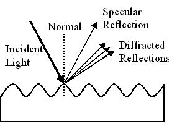
The other phenomena that propagating waves experience is diffraction. It is the spreading out of waves. All waves tend to spread out at the edges when they pass through a narrow gap (for distances that are comparable to the wavelength of the electromagnetic wave) or encounters an object. Instead of saying that the wave spreads out or bends round a corner, it is commonly referred as the wave is diffracted around the corner.
Intuitively, the longer the wavelength of a wave, the more it will diffract. Another important remark is that the diffraction loss increases with increasing frequency. A familiar example from daily life is the reflection of image on a compact disc (CD) or digital versatile disc (DVD). Here, the surface of a CD/DVD acts as a diffraction grating for the reflection of images incident on its surface. This is the main reason that when one looks at the back of a CD/DVD, the tracks of it act as a diffraction grating and produce iridescent reflections of the sunlight. Another example from daily life is the color of spider webs.
2.1.3 Scattering
The obstacles or inhomogeneities in the medium force to deviate the propagation of light from its straight trajectory. When the light is scattered by one large scatterer, then it is called single scattering and similarly, when there are several sources of scattering in the medium that interact with the light, then it is named as multiple scattering. Mathematically, single scattering is treated as random since the location of the single scatterer in the propagation path is not known whereas multiple scattering is considered to be deterministic since the random nature of several scatterers can be averaged out. An example for single scattering is when an electron is sent to an atomic nucleus. The exact position of the nucleus relative to the electron is not known and this bring the random nature of this interaction. To solve these type of problems, in most cases, probability distributions are used to describe single scattering. A light passing through a thick fog can be given as an example for multiple scattering. Several models are proposed in literature to model scattering coefficients depending on the environment [25] such as Rayleigh scattering where the inhomogeneities in the medium are small compared to the wavelength of the light, Mie scattering where both sizes are comparable to each other and non-selective scattering where the obstacle size is much larger than the wavelength of the light. Rayleigh scattering is the reason that the sky is blue in the day time and reddish in the sunset. Mie scattering occurs on the lower portions of the atmosphere where the clouds overcast the sky and the abundant particles are large. Non-selective scattering is the reason that the fog and clouds look white since each color of the light is scattered around in equal portions resulting in white color.

2.2 The IEEE 802.15.3a Standard Channel Model
This model aims to capture the multipath characteristics of typical indoor environments where IEEE 802.15.3a devices operate. In addition to the UWB channel measurements performed mainly in 2002, a number of measurement campaigns were carried out by the participants of the task group [26]. Throughout these campaigns, three channel models were considered in general: Tap-delay line Rayleigh fading model, the Saleh-Valenzuela (S-V) model and the -K model and these are summarized in [23] and [27].
The experimental measurements indicate that the transmitted signals through multipath RF environments arrive to the receiver as clusters. The proposed UWB channel model is based on the cluster approach first proposed by Turin and others in 1972 [28] and further formalized by Saleh and Valenzuela (S-V model) which was proposed in 1987 [29] only with one significant modification. It was experimentally observed that when lognormal distribution is used to model multipath gain magnitude instead of Rayleigh distribution, it would better fit to measurement data.
The S-V model which assumes the multi-path components of the same pulse arrive as clusters, the time of arrival of these clusters are modelled as Poisson arrival process with rate
| (2.1) |
where and are the arrival times of the and clusters, respectively. The arrival time of the first cluster is usually set to zero, . Similarly, within each cluster, consecutive multi-paths arrive with a Poisson arrival process with rate
| (2.2) |
where and are the arrival times of the and paths (rays) of the cluster, respectively. As again, the arrival times of the first rays within each cluster is set to zero, for . Having defined the arrival rate processes, the proposed IEEE 802.15.3a multipath model has the following discrete-time impulse response
| (2.3) |
where denotes the log-normal fading random variable, and denotes the number of observed clusters and multipaths within each cluster, respectively. is the delay of the cluster and denotes the channel coefficient of the cluster multipath. The channel coefficients can be further can be represent by
| (2.4) |
where is a Bernoulli random variable taking equiprobable values of and it takes account for the signal inversion due to reflection. The other random variable, is the log-normal distributed channel coefficient that belongs to the cluster of path. This coefficient is expressed as
| (2.5) |
where is a Gaussian random variable with mean and variance and can further represented as
| (2.6) |
where and are two Gaussian random variables representing the fluctuations of the channel coefficient on each cluster and on each contribution, respectively. The variances of these two random variables are represented by and , respectively. The first term on the right hand side in (2.6), is closely related to the exponential power decay factors of amplitude of the clusters and multipath by
| (2.7) | |||||
| (2.8) |
where is referred to as normalization factor of the total received power and sometimes denoted by for simplicity. Often in communications, in order not to amplify or attenuate the transmitted signal, the channel coefficients are normalized to unity for each realization in the system model and it requires that
| (2.9) |
Once again, let us remark that the arrival times of each cluster and each multipath within a cluster is modelled by two Poisson process which were previously defined in (2.1) and (2.2).
The amplitude gain is also assumed to be a log-normal r. v. with the relation where is a normal random variable with mean and variance . The mean depends on the average total multi-path gain and expressed as
| (2.10) |
where stands for the natural logarithm. is dependent on average attenuation exponent by
| (2.11) |
where is the reference power gain evaluated at . is the path loss at a reference distance in dB. In literature, this is sometimes denoted as and it is related to reference value for power gain by
| (2.12) |
In 2003, based on several experimental results, Ghassemzadeh and Tarokh suggested values for dB and to be used in line-of-sight (LOS) environment and dB and in NLOS environment [30]. Using these definitions, the parameters for IEEE 802.15.3a UWB channel model can be summarized in Table 2.3.
| Parameter | Definition |
|---|---|
| Average arrival rate of clusters | |
| Average arrival rate of multipaths with in clusters (rays) | |
| Power decay factor for clusters | |
| Power decay factor for rays within clusters | |
| Standard deviation of the fluctuations of the | |
| channel coefficient for clusters | |
| Standard deviation of the fluctuations of the | |
| channel coefficients for rays within clusters | |
| Standard deviation of the channel amplitude gain |
Since different in-door environments exhibit different channel characteristics and the channel parameters need to be updated. These different characteristics arise from several facts. Depending on the distance between the transmitter and receiver and whether a LOS component exists or not several channel model scenarios are been proposed. The first scenario, channel model 1 (CM1) is valid for distances of meters with LOS component. The second scenario, CM2 is valid for the same distances but it considers NLOS cases. For distances of meters with NLOS cases, CM3 is used. The final scenario, CM4 is the one that includes extreme NLOS case. The channel model parameter values for these four channels are given in Table 2.4.
It should be emphasized that since this is a discrete-time impulse response model, the time resolution of the system plays a crucial role. Table 2.4 correspond to a time resolution of 167 psec which corresponds to a bandwidth of 6 GHz. Therefore, for any other time resolution, scaling in time domain is needed for each of the channel coefficient realizations.
| Scenario | ns | ns | (ns) | (ns) | (dB) | (dB) | (dB) | |
|---|---|---|---|---|---|---|---|---|
| CM1 | 0.0233 | 2.5 | 7.1 | 4.3 | 3.3941 | 3.3941 | 3 | |
| LOS (- m) | ||||||||
| CM2 | 0.4 | 0.5 | 5.5 | 6.7 | 3.3941 | 3.3941 | 3 | |
| NLOS (- m) | ||||||||
| CM3 | 0.0667 | 2.1 | 14 | 7.9 | 3.3941 | 3.3941 | 3 | |
| NLOS (- m) | ||||||||
| CM4 | 0.0667 | 2.1 | 24 | 12 | 3.3941 | 3.3941 | 3 | |
| Extreme NLOS |
Chapter 3 FREE-SPACE OPTICAL SYSTEMS
Free-space optical (FSO) systems are originally created to supplement fiber-optical cable systems and their apparatus and techniques originate from fiber-optical systems. Digital information in the form of binary signals are sent through building roofs or window-mounted infrared laser diode transmitters. Usually, the systems use narrow optical pulses to transmit ’s and transmits nothing for ’s and this type of modulation scheme is called On-Off Keying (OOK). Another common modulation technique in FSO systems is pulse position modulation (PPM) where there are pulse slots of duration. Depending on the position of the pulse, typically equal energy pulses are transmitted. In this scheme, synchronization between transmitter and receiver plays an important role to determine the starting positions of the pulses. Transmission efficiency is enhanced by packetizing data which ensures that dividing traffic into packets that can be independently sent and received. Also, similar to many fiber-optical communications, FSO can support wavelength division multiplexing (WDM) which allows a single optical path to carry different signal channels ensured that each signal has a different wavelength.
Typically, and nm laser diodes are the common commercially available products in today’s technology. In these systems, the information is transmitted by modulating the signal intensity denoted by which is produced in response to an input electrical current signal and this process is called intensity modulation. It is important to emphasize that the information in these systems are carried in the intensity of the transmitted signal contrary to the RF systems where either the amplitude, the frequency or the phase of the signal or sometimes any combination of these are used to transmit information. The generated optical intensity is focused by a lens and released out as a beam of light just like flashlights. Although these pulses are focused by a lens, the power of the beam still disperses over long distances. At the receiver, the transmitted light is focused back onto a photodetector which generates current proportional to the intensity incident on its photodetector area and this process is called direct-detection. This process inside the photodetector is analogous to square law devices for RF systems where the integral of the amplitude square of the signal is taken over a time period. In many cases, the generated current in the photodetector is weak and amplification is employed in the receiver end before it is demodulated. By this way, optical to electrical conversion of the signals are accomplished.

Due to the underlying structure of the channel, types of modulation and detection of optical signals are limited to variations on the optical intensity. This imposes the non-negativity constraint on the signals to be transmitted and this can be shown as
| (3.1) |
and the above constraint is meaningful in the sense that the transmitted power can physically never be negative [31]. Here, it should be emphasized that the received signal in the photodetector that is shown by
| (3.2) |
where is the modulating data and denotes the noise in the system, can take negative values depending on the noise characteristics.
Another important physical characteristics in FSO systems is beam divergence. The transmitted beam diverges by the time it arrives at the receiver. The degree of beam spreading depends on the lens diameter and the received energy at the collecting lens decreases with the square of the link distance. Without investigating the atmospheric conditions, transmit optical power, receiver sensitivity and size of the collecting lens, all impose constraints on the range of the communication link for a given data rate [32].
In order to increase the range of the communication link, the diameter of the transmitting lens needs to be increased. By employing larger lens diameters, the power incident on the collecting lens is increased resulting in reduced beam spreading. Although there are physical limitations on how large the lens diameter can be, there is also another problem associated with using large lenses. As the diameter of the lens gets larger, the beam spreading gets narrower causing the alignment between transmitter and receiver to get difficult. Including the building sway effects and thermal expansion or contraction of tall buildings, focusing may cause problems due to narrow beams. Therefore, many commercial products employ auto-tracking capabilities to both ends which brings additional cost and complexity to the system. To deploy tracking capabilities to FSO systems, movable mechanical platforms or sometimes articulated mirrors are used to ensure correct pointing of the transmitted beam.
Atmospheric weather conditions such as fog, rain and snow are the other factors that limit the range of FSO links. Among these weather conditions, FSO systems are most susceptible to fog. For example, in moderate dense fog, the optical signal loses 90 percent of its strength every 50 meters so for a link distance of 150 meters 99.9 percent of the transmitted optical energy will be dissipated [32]. Therefore, while deploying FSO systems, weather conditions of the deployment cites need to be carefully investigated.
To solve the range versus reliability problem for FSO systems, they are designed with limited link lengths to form an optical mesh topology. By this way, when several links fail, the spider web like structure may still ensure the signal to be redirected through a different path ensuring availability of the service. On the other hand, the mesh topology brings complexity to the system. To control the distribution of the signals along the paths, network management type systems are needed.
3.1 Free-Space Optical Channels
In order to fully design and analyze the properties of a communication channel, the propagation characteristics of the path from transmitter to receiver must be taken into account. Therefore, electromagnetic propagation of the waves needs to be investigated. There are two types of propagation depending on the medium such as guided and unguided transmissions. In guided channels, wave guides are used to confine the wave propagation from transmitter to receiver. Fiber-optical cables are the primary examples for such communication systems. On the other hand, in an unguided channel, the transmitter releases the generated field freely into a medium without any attempt to control its propagation except to control its antenna gain pattern. This unguided channel is often called as space channel and common examples of this channel are free space, the atmosphere or the ocean (underwater) [8]. Unfortunately, the characteristics of unguided (space) channels primarily depend on the properties of the medium. Free-space channels are the simplest type of unguided channels where the medium between transmitter and receiver is free-space.
In FSO links, inhomogeneities induced by the temperature and atmospheric pressure cause fluctuations in the received light intensity [5] which lead to turbulence induced fading. Depending on the characteristics transmission path, this type of fading may be severe and thus, limit the performance of the communication system by increasing the link error probability. Also, weather conditions such as fog, rain and snow can lead to aerosol scattering and degrade the performance of FSO links and these effects are discussed in [33] and [34].
In FSO communication systems, there are two parameters that describe turbulence-induced fading such as the correlation length of intensity fluctuations, and the correlation time of intensity fluctuations denoted by . These two parameters closely effect the link performance by imposing constraints on aperture diameter and bit duration. If the diameter of the receiver aperture denoted by is larger than the correlation length, then turbulence-induced fading can be reduced significantly by employing multiple point receivers in the receiver side and this technique is called aperture averaging [10]. Since can not be always satisfied, to mitigate the effects of fading, several approaches have been proposed in [5]. These approaches include temporal-domain and spatial-domain techniques. To reduce the effects of fading by temporal-domain techniques is maximum-likelihood (ML) symbol-by-symbol under the assumption that the receiver has the knowledge of marginal fading but does not have the temporal fading correlation nor the instantaneous fading states. When the receiver knows the joint temporal fading distribution but no the instantaneous fading state, the receiver can employ MLSD. As spatial-domain techniques, multiple receivers must be employed at the receiver to collect the incident intensity. As in radio frequency communication systems, receivers need to be separated as far as possible in order to maximize the receive diversity gain. Therefore, uncorrelated turbulence induced fading can be achieved. In practice, separating receivers may not be made possible due to the large area they would occupy and then correlated turbulence fading would occur. Techniques to mitigate the above mentioned turbulence induced fading effects in temporal and spatial domain are explained in [5].
An important parameter in Kolmogorov theory is refractive index and it is defined as [5]
| (3.3) |
where defines the average index and denotes the fluctuation component induced by spatial variations of both temperature and pressure. The autocorrelation function of , represents the spatial coherence of the refractive index denoted by . its Fourier transform denoted by is called wave number spectrum and it can be represented as
| (3.4) |
where denotes the Fourier transform operation.
According to Kolmogorov theory, turbulence characteristics can be divided into three regions.
- •
Input Range: This region considers the case when the eddy size is greater than outer scale of turbulence , ie, (eddy size). In this region, the turbulence is anisotropic and the wind shear and temperature gradient introduces energy to the turbulence. Since the energy sources may vary, no general formula is applicable to this chaotic region [35].
- •
Inertial subrange: This region considers the case when the eddy size is between the inner and outer scale of turbulence, ie, (). In this region, the turbulence is fairly isotropic and the kinetic energy of the eddies dominates the energy due to the viscosity dissipation.
- •
Dissipation range: This region considers the case when the eddy size is smaller than the inner scale of turbulence, ie, (). In this region the energy due to the viscosity of eddies dominates the kinetic energy.
Depending on the ranges, the Kolmogorov wavenumber spectrum can be found differently. Unfortunately, for the input range, the spectrum is still unknown [35]. For inertial range, it can be given by
| (3.5) |
where is the wavenumber spectrum structure parameter and it is an altitude-dependent parameter. For dissipation range, the spectrum is considered to be zero, ie, . The following formula is often considered to characterize all three regimes
| (3.6) |
where . This equation is referred to as von Karman spectrum. Using Hufnagel and Stanley model, the wavenumber spectrum structure parameter can be given by [35]
| (3.7) |
where describes the strength of the turbulence and is the effective height of the turbulent atmosphere. Several works in literature define the wavenumber spectrum structure parameter as [6, 11]
| (3.8) | ||||
where is altitude in meters, is the root mean square (rms) of the wind speed in meters per second and A is the nominal value of at the ground and its unit is . The wave number spectrum structure parameter, can vary from for weak turbulence regime to for strong turbulence regime. A typical average value is assumed to be in [9].
This work assumes that the energy of large scale eddies are redistributed without loss to eddies of decreasing size until finally dissipated by viscosity [5]. Therefore, the size of turbulence eddies may vary from millimeters to meters. Denoting the inner and outer scale of the eddies by and , respectively, when the link distance satisfies the following condition
| (3.9) |
where is the wavelength of the transmitted signal, and are defined as above, then the correlation length of the fading channel, can be approximated by [10]
| (3.10) |
where denotes the Fresnel zone of the turbulence. Here, it needs to be mentioned that, the above equation does not take into account of aerosol effects such as rain and snow. These effects would further degrade the coherence of the optical field and lead to decrease in the correlation length of the fading channel. In literature, “frozen air” model is used while modelling the behavior of the eddies in the atmosphere. As the name suggests, this model assumes that the eddies present along within the path preserve their relative location to each other.
3.2 Statistical Models of Turbulence Regimes
In FSO channels, depending on the strength of atmospheric turbulence the distribution of light intensity is categorized into three regimes such as weak, moderate and strong turbulence conditions. All these conditions are represented via distinct distributions that accurately model the channel fadings under the associated regime. The weak turbulence is represented by log-normal distribution, moderate turbulence is described by gamma-gamma distribution and at the extreme case, strong turbulence is denoted by negative exponential distribution. These statistical models will be analyzed in detail in the following subsections.
3.2.1 Weak Turbulence Conditions
The emitted light from the transmitter propagates through large number of elements of the atmosphere and at times where each element on the propagation path causes independent, identically distributed (i.i.d.) scattering and phase delay, the central limit theorem (CLT) can be invoked to represent the marginal distribution of log-amplitude fluctuations that will be represented by and its distribution can be shown as
| (3.11) |
where denotes the ensemble average of log-amplitude fluctuations and denotes its variance. Commonly, it is assumed that the light intensity represented by the random variable, is related to the log-amplitude by [5]
| (3.12) |
Then, the marginal distribution of the light intensity can be expressed as
| (3.13) |
The variance of log-amplitude fluctuations of plane and spherical waves can be found using the following equations [5, 9]
| (3.14) | |||||
| (3.15) |
where is the wavenumber spectrum structure parameter as described previously, and is the propagation path between the transmitter and receiver. Also, below expression is commonly use to relate scintillation index and variance of log-amplitude fluctuations such that
| (3.16) |
Although above expressions can handle varying wavenumber spectrum structure parameter, in this work, it is assumed to be constant along the horizontal path. On the other hand, in some references such as [4, 11, 17], the log-normal distribution of the light intensity has a similar representation which uses the Rytov theory, and it is given as
| (3.17) |
where denotes the aperture-averaged scintillation index. Depending on the wave characteristics, the scintillation index for a plane wave and spherical wave can be expressed as
| (3.18) | ||||
| (3.19) |
where and are the Rytov variance for a plane wave and spherical wave, respectively, , D is aperture diameter, is the wave number given by , and the parameters and are given as above. In cases where only a single point detector is used, ie, aperture averaging is not employed, is taken as zero since the propagation path, , is much larger than the diameter of a single detector, . Finally, although using the relation between light intensity and Rytov variance is widely used as in [4, 17], it is not considered in this work under the weak turbulence conditions but similar expressions invoking Rytov theory under moderate turbulence conditions are considered in following section.
In the following two figures, the close relation between standard deviation of log-amplitude fluctuations, and path distance, is shown. Using (3.14) and (3.15), as the link distance varies from hundred meters to a kilometer, the standard deviation of log-amplitude fluctuations increase from to . This general behavior is depicted in the figures and the wavelength of the optical transmitted wave is taken as 1550 nm and is assumed to be constant throughout the link distance.


3.2.2 Moderate Turbulence Conditions
Under moderate turbulence conditions, both the small and large scale scatterers are effective and the intensity fluctuations are modelled by the Gamma-Gamma distribution described by the following probability density function
| (3.20) |
where and are the Gamma function and the th-order modified Bessel function of the second kind, respectively [36]. Small and large scale scattering effects that are represented by and , respectively in (3.20) are related to the atmospheric conditions for a plane wave with aperture-averaged scintillation index by [10]
| (3.21) |
where is the Rytov variance for a plane wave, , D is aperture diameter and the parameters , and are given as above. The same parameters are related to atmospheric conditions for a spherical wave with aperture averaging by
| (3.22) |
where (ie, ) is the Rytov variance for a spherical wave and the other parameters, and are as defined previously. These parameters are related to the scintillation index by and moderate turbulence regime is often assumed to be valid for .
Increase in the link distance or increase in the wavenumber spectrum structure parameter would result in an increase in the Rytov variance for each type of waves, and . Using this fact and the above equations to determine small and large scale effects, the following figure is plotted to depict the relation between link distance and parameter pairs. For small link distances, both small and large scale scattering effect parameters and have large values and as the link distance increases small scale scattering effects significantly increases after some point whereas large scale scattering effects constantly decrease and approach to unity. For the scintillation index, this parameter always increases and reaches a saturation limit as the link distance gets larger. This saturation regime is better described by negative exponential distribution which is explained in the next subsection.

3.2.3 Strong Turbulence Conditions
Under strong turbulence conditions, there are many non-dominating scatterers in the medium. Passing from medium to strong turbulence regime corresponds to the case when the small scale scattering effects denoted by increase but the large scale scattering effects approach represented by approach to unity as the link distance increases and under this condition, the light intensity is better modelled as one-sided negative exponential distribution which is given by
| (3.23) |
where denotes the mean light intensity. This saturation regime corresponds to scintillation index for the range . To show that gamma-gamma distribution converges to negative exponential distribution in the saturation regime the following figure is plotted. For the same pairs in the previous subsection, the pdf’s are depicted in Fig. 3.5. As the link distance increases approaches to unity and grows unboundedly. This behavior is depicted in the figure such that the longest link distance which is shown as the red curve has a negative exponential distribution. Aside from this mathematical interpretation, physically in the saturation regime large scale effects are not dominant instead there are several non-dominating small scale scattering effects are effecting the propagation of light.

Chapter 4 PROPOSED ULTRA-WIDEBAND SYSTEM AND ITS ANALYSIS
The proposed system model in this work includes two separate sections such as free-space optical (FSO) and radio-frequency (RF) system models. Both of the systems employ ultra-wideband signalling to achieve very high data rates. The FSO system is designed such that it can take binary inputs in both electrical or optical domain. These inputs are used to generate optical pulses and transmitted via FSO links over several kilometers. The received signals are demodulated in the receiver and they can be used right away since they are converted to electrical domain using the photodetectors in the receiver. The main advantage of this section of the system is to reduce the time and cost to install fiber optical cables for long distances since both the installation time and cost to deploy FSO equipment is much shorter and cheaper compared to deploying fiber optical equipments. Also, depending on the link design, the received estimates of the FSO links can be used to distribute the information inside the buildings. Using simple and commercially available UWB transmitter and receiver pairs, the information can be delivered to the end-user in the last-step. Due to the severe attenuation of the signal in the RF domain, the distance between the transmitter and receiver in the last-step is limited to short distance up to 10 meters. For both sections of the system, their systems models are presented and their detection error probabilities (DEP) are analyzed in the following sections. The FSO system performance is closely related to the atmospheric turbulence conditions. Therefore, its performance analysis is divided into three parts depending on the strength of the turbulence such as weak, moderate and strong conditions. Also, simulations are carried out to verify the derived theoretical results. Towards the end of this chapter, channel capacity analysis of the FSO system is presented.
4.1 System Models

4.1.1 Free-Space Optical System Model
The system model shown in Fig. 4.1 is considered and the approaches presented in [37] and [38] are adopted. The proposed system employs gain-switched Fabry-Perot laser diode (FPLD), a tunable-filter (TF) and an erbium-dope fiber amplifier (EDFA) to generate wavelength-tunable optical pulses and is primarily developed for UWB-over-fiber links. In the system model, the binary source outputs ’s are time-hopping pulse-position modulated (TH-PPM) via Gaussian pulse trains and passed through a bias-tee circuit to drive the FPLD into gain-switched operation. The -nm FPLD, which operates with a threshold current of mA at C with nm mode spacing is biased at mA and gain-switched at GHz. The generated optical signal is fed to the EDFA which consists of a -nm pump laser diode that pumps mW output power to couple an erbium-doped fiber via -nm wavelength division multiplexer (WDM) and an isolator to reduce back reflections and serves both as an external-injection source and an amplifier for the FPLD output. The output of EDFA is passed through TF which operates in the range from to nm. The central wavelength of the TF is chosen to be close to that of FPLD output so that the system has a single wavelength output before it is sent to FSO channel. The generated optical TH-PPM signal can be represented as
| (4.1) |
where denotes the pulse energy amplified by EDFA, denotes the Gaussian pulse, and are the binary information and pseudo-random code sequences for time hopping, respectively. , , and represent the symbol, bit, chip and pulse durations, respectively and bits are repeated times in a symbol period.
The FSO channel is described by the unit impulse response where and are the instantaneous light intensity and the background radiation whose effects are removed at the receiver as in [5], respectively. Also, experiments show that the coherence time of the FSO links is large enough to approximate the intensity as a constant during the transmission of a frame, i.e., .
The photo-detector receives the photon flux incident on the detector area and produces a current that is proportional to the received photons, providing the optical to electrical conversion of the received signal. The conversion coefficient () indicates the efficiency of the photodetector. After the removal of the background radiation bias , the resulting received signal can be represented as
| (4.2) | |||||
where represents the combined effects of both the thermal noise and the shot noise, which can jointly be modelled as an additive white Gaussian noise (AWGN) with zero mean and variance , i.e., . The received signal is passed through the matched filter which can be written as
| (4.3) |
resulting in the sampled output
| (4.4) |
Here, the noise term is also AWGN with . To make decisions on the sampled output values zero-threshold detection is employed for the matched filter outputs. The estimates of these binary source outputs, ’s are then input to an UWB transmitter to be transmitted to the end-user.
4.1.2 Radio-Frequency System Model
In this subsection, radio-frequency section of the system model is considered. It should be emphasized that this part of the system constitutes the last-step to the end-user. The TH-PPM pulse that is generated by the UWB transmitter can be expressed as
| (4.5) |
where denotes the energy of the pulse, denotes the Gaussian monocycle pulse train satisfying the UWB regulations. The UWB channel is modelled as
| (4.6) |
where denotes the log-normal fading random variable, and denotes the number of observed clusters and multipaths within each cluster, respectively. is the delay of the cluster and denotes the channel coefficient of the cluster multipath and it can be expressed as where is a Bernoulli random variable taking values of and is the log-normal distributed channel coefficient. To normalize each channel realization to unity requires that
| (4.7) |
The amplitude gain is also assumed to be a log-normal r. v. with the relation where is Gaussian distribution with mean and variance . The mean depends on the average total multipath gain and expressed as
| (4.8) |
where is the natural logarithm. is dependent on average attenuation exponent by , and is the reference power gain evaluated at . denoting the path loss at a reference distance in dB is related to by . Assuming the transmission of the Gaussian monocycle pulse train defined in (4.5), the received signal can be expressed as
| (4.9) | ||||
Using an UWB receiver, estimates of the signal that passed through FSO and RF links, ’s are obtained.
4.2 Detection Error Probability Analysis
In this section, the error probability of the composite system including the introduced by both FSO and RF links is presented. The total error probability of the complete hybrid system is denoted by and it can be expressed as
| (4.10) |
where , and , are the error probabilities and symbol signal-to-noise ratios of the FSO and RF systems, respectively. Since binary TH-PPM is employed, the above equation includes errors introduced by both FSO and UWB links of the composite system. Although the primary scope of this work is to analyze the FSO system performance for different channel regimes but also, the performance analysis of the RF channel is briefly investigated and is presented along with the analysis of the FSO channel.
The detection error probability (DEP) for the binary TH-PPM signal model over FSO subsystem assumes perfect synchronization between the transmitter and receiver. Also, channel state information (CSI) is assumed to be available at the receiver. Thus, the detection error probability can be expressed as
| (4.11) |
where is the complementary error function and is the average pulse signal-to-noise ratio (SNR) and denotes the expectation operation. Notice that due to the random fluctuations in its amplitude, the light intensity is modelled as a random variable whose distribution is dependent on the turbulence region. Expectation is taken over the distribution of the light intensity to find the average DEP such that
| (4.12) |
4.2.1 Error Probability Under Weak Turbulence Conditions
Under weak turbulence conditions, the average DEP can be computed by taking the expectation in (4.12) over the log-normal intensity distribution in (3.13) such as
| (4.13) |
Unfortunately closed form solution of the above equation does not exist, but via Gauss-Hermite expansion in [39] which is given by
| (4.14) |
where and , , are the root (abscissa) and associated weight, respectively, (4.13) can be approximated after a change of random variables as
| (4.15) |
As shown in the simulation results, the Gauss-Hermite expansion up to order whose parameters given in [39] provides a close approximation to the actual integral in (4.13).
4.2.2 Error Probability Under Moderate Turbulence Conditions
Under moderate turbulence conditions, the average DEP can be computed by the expectation in (4.12) over the Gamma-Gamma intensity distribution given in (3.20) such as
| (4.16) |
Using the formulation in [40] the integrands and in (4.16) can be expressed in terms of Meijer’s G-function and rewritten again as
which, using Eq. 07.34.21.0011.01 of [40], results in a closed-form expression such that
The intermediate steps in deriving the above closed-form expression are presented in Appendix B.1.
4.2.3 Error Probability Under Strong Turbulence Conditions
4.2.4 Error Probability in Coded FSO Links
The system proposed in Fig. 4.1 can also be implemented with a channel encoder-decoder pair to protect the information bits transmitted over the FSO channel against channel effects. If a convolutional encoder is employed together with the Viterbi decoding on the receiver side, the coded bit error probability in terms of the uncoded error probability is expressed approximately as in pp. 531 of [41]
| (4.24) |
where is the minimum free distance of the convolutional code, and is the sum of the Hamming weight of all the input sequences whose associated convolutional codeword have a Hamming weight of .
4.2.5 Error Probability in RF-UWB Links
Assuming normalized channel coefficients, i.e., (4.7) holds, the received SNR at UWB receiver can be expressed as , where denotes the average pulse SNR and results in the following error probability . Averaging out the pdf of over results in
| (4.25) |
This can be solved by Gauss-Hermite expansion as in (4.14) after a change of variables as
| (4.26) |
where and are as defined earlier.
4.3 Simulation Results
In this section, simulation results for the error performance of the proposed FSO-UWB system under weak, moderate and strong turbulence conditions and for the hybrid system including the RF section in the last-step are presented. For the simulations, frame size, repetition rate and the efficiency of the photo-detector are chosen as symbols, and , respectively.
For each turbulence condition, it is assumed that is constant through the horizontal path and for weak turbulence, it is taken as . For link distances over 2, 2.5, 3 and 4 km, these correspond to and , respectively. The analytical approximation derived in (4.15) and the Monte-Carlo simulations are shown in the group of first 4 BER curves in Fig. 4.2. As seen in the figure, the theoretical derivations, represented with dashed-lines show a good correspondence to the simulated performances, depicted in solid lines.
For moderate turbulence condition, the wavenumber spectrum structure parameter is taken as and consider link distances over 2, 2.5 and 3 km. Using the relation in (3.21), the parameter pairs are , and , respectively. The simulation results in Fig. 4.2 for all three cases are in full accordance with the exact closed form expressions given in terms of the Meijer’s G-function.
For strong turbulence, unit mean light intensity is assumed, and . The analytical and the Monte-Carlo simulated results are shown in the figure and as expected, the system exhibits the worst performance in this case due to the saturation characteristics in this regime.


In Fig. 4.3, the transmission of the detected optical signals through a LOS RF UWB channel in the last-step to the end-user is considered. The parameters for LOS channel model, CM1 are taken as dB, dB and [30, 42] and the RF link distance is taken as 2 meters. For the FSO link, we assume that the signals are transmitted over 2 km at 30 and 45 dB. Under weak and moderate conditions, is again chosen as and which corresponds to and , respectively. The results are shown in Fig. 4.3 where the thick dashed curve shows the performance of the RF UWB transmission over CM1 channels only. The rest of the curves consider the case where the detected bit values are transmitted over the FSO channel. Therefore, these curves represent the combined error performance over both the FSO and the RF sections of the transmission link. Notice that the hybrid system performance exhibits error floors resulting from the errors introduced in FSO links. However, if the SNR over the FSO link is over dB, the error floor for weak turbulence is significantly low. This indicates at this or higher SNR, under weak turbulence, the hybrid system increases the UWB signalling range to 2 km without any sacrifice in the performance. Similar results can be achieved for moderate turbulence conditions, if the FSO channel SNR is dB or more. Unfortunately, for the extreme case of strong turbulence, the error floors appear high even at large SNR values.
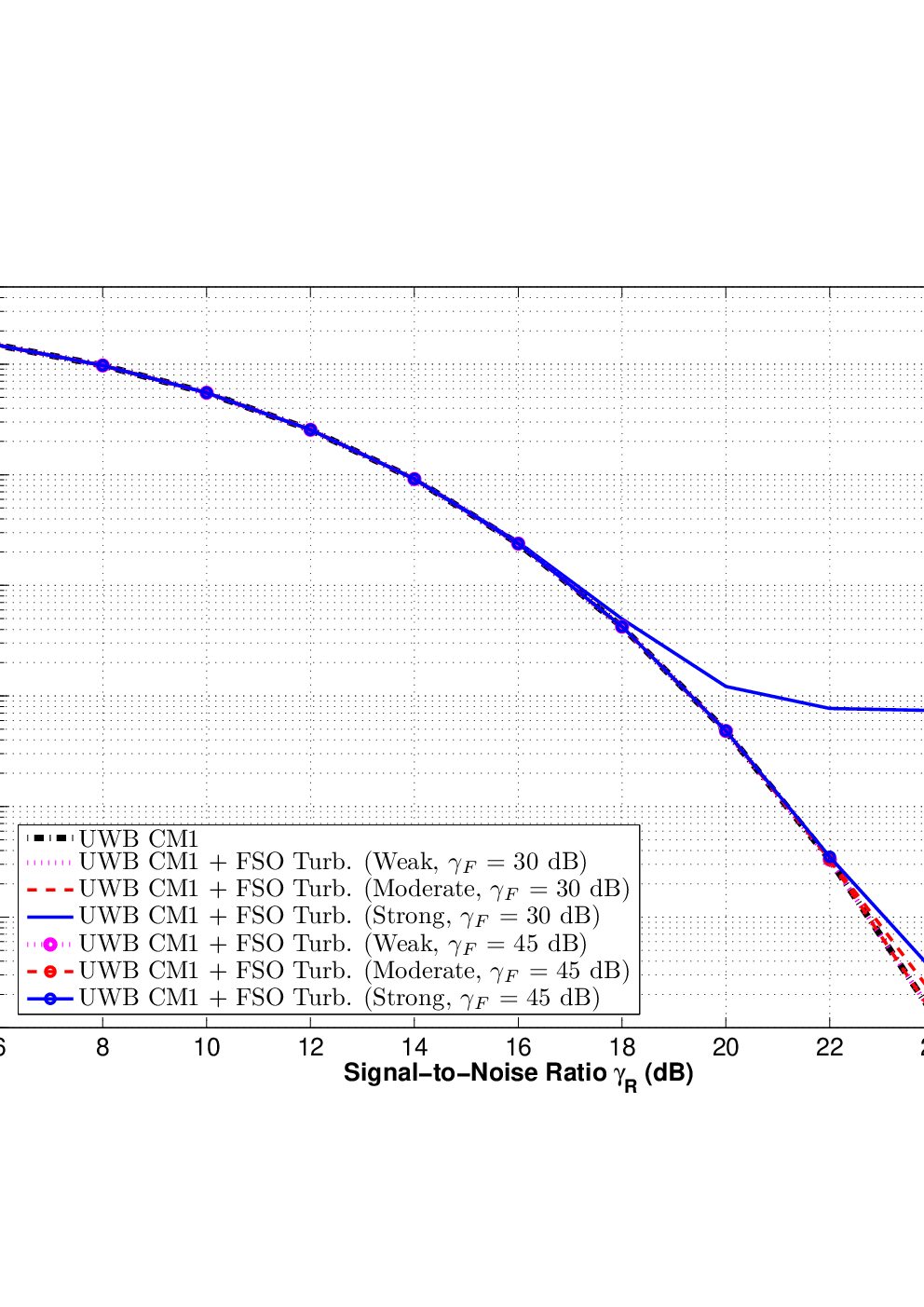
To lower these error floors, we consider the case when a simple convolutional encoder/Viterbi decoder pair within the FSO subsystem is employed. With this addition, the errors introduced in the FSO links are reduced to improve the overall system performance. A rate convolutional code with generator and , ([41], pp. 540) is employed together with a Viterbi decoder. The coded system performance under each turbulence regime is shown in Fig. 4.4 and only the error floors under strong turbulence conditions are shown for comparison purposes with uncoded signalling scheme. Notice that the use of even a very simple code reduces the error floors significantly. For instance, the error floors for the strong turbulence condition at dB is for the uncoded system whereas it is reduced significantly down to when coding is employed. Table 4.1 shows the error floors in both cases for each turbulence condition. Thus, at the cost of additional complexity introduced by Viterbi decoder, the error floors of the uncoded system performance is significantly lowered.
| Weak | Moderate | Strong | ||
|---|---|---|---|---|
| Uncoded | ||||
| dB | Coded | |||
| Uncoded | ||||
| dB | Coded |
4.4 Channel Capacity Analysis
In his pioneering work in 1948, Claude Shannon introduced the term “channel capacity” where the bandwidth and the signal-to-noise ratio together determine the quality of a transmission channel [43]. Until that moment, this relation was not seen. In his works, the capacity of a noisy channel is defined as the maximum possible transmission rate at which reliable communication over the channel is possible [22]. For transmission rates that are lower than the channel capacity , one can always design codes that achieve arbitrarily small error probabilities. Hence, for a discrete memoryless channel, the average channel capacity can be expressed as
| (4.27) |
where denotes the mutual information between the random variables and which are commonly referred as the channel inputs and channel outputs, respectively. The probability distribution function denoted by represents the channel variations. The average capacity of a power-limited AWGN channel is given by
| (4.28) |
where and denote the power of the signal and noise, respectively and shows the signal-to-noise ratio (SNR). In this form, the capacity is in bitssecHz units if the logarithm is taken in base 2 and in natssecHz units if the natural logarithm is used. For a given bandwidth , the same channel capacity can be represented as
| (4.29) |
and in this form, its is in bitssec units since the bandwidth is used in the equation. For different channel variations, the above can be revised to include the effects of channel that are represented by as
| (4.30) |
This means that the average capacity of a fading channel is found by taking the expectation of the AWGN channel capacity over the fading term. This is reasonable to make a comparison between the channel capacity of any fading channel and AWGN channel. The former is always greater or equal to the latter capacity and to prove this Jensen’s inequality can be used such as
| (4.31) |
and using the above equation, it can be concluded that the average capacity of an AWGN channel is an upper bound to any fading channel capacity. In the following subsections, the average capacity of the proposed free-space optical link is investigated under weak and moderate turbulence conditions.
4.4.1 Channel Capacity Under Weak Turbulence Conditions
On the propagation path of the transmitted light in FSO channel, there are several inhomogeneities in the atmosphere which independently lead to distributed phase delay and scattering. Using this and invoking the Central Limit Theorem (CLT) then is Gaussian distributed random variable with mean and variance . These inhomogeneities in the atmosphere are related to the received light intensity by
| (4.32) |
Here, it needs to be mentioned that in previous sections the above equation included the mean term where in this section it is ignored to include its effects in the closed-form expression of the channel capacity. The marginal distribution of the light intensity can be represented as
| (4.33) |
Taking the expectation over the pdf of received light intensity would result in
| (4.34) |
Applying change of variables such that then . Hence,
| (4.35) |
Completing the squares in the exponential term would result in
| (4.36) |
Consider the case when the fading does not attenuate or amplify the average power, then normalizing the fading coefficient such that would require to choose the mean of the log-amplitudes to be [6]. Under this condition, the average capacity of the log-normal channel can be calculated as
| (4.37) |
The above expresses the capacity in bitssec units since the logarithm is taken in base and the bandwidth of the message is considered in the equation. Applying change of variables such that , then (4.37) becomes
| (4.38) |
Integrals of this form can be approximated via Gauss-Hermite expression form as in (4.14). Then, rewriting (4.38) will result in
| (4.39) |
where and are as described in previous section.
4.4.2 Channel Capacity Under Moderate Turbulence Conditions
The channel capacity of an FSO link under moderate turbulence conditions is calculated by solving
| (4.40) |
where the pdf of the light intensity under moderate conditions is used in the integration. For the above equation, applying change of random variables such that and Meijer’s G-function representations of the integrands and , it can be written as
This form can be further simplified to a closed-from expression such as
| (4.45) | ||||
where the intermediate steps to derive the above closed-form expression are shown in Appendix B.2 in detail.
In Figure 4.5, the average channel capacity of the FSO link is presented. Depending on the turbulence conditions, different fading effects are investigated. Under weak and moderate turbulence conditions, the average channel capacity of the FSO system are plotted. The wavelength is taken as nm and the wavenumber spectrum structure parameters for weak and moderate turbulence are taken as and , respectively. The link distances of and are considered in the figure. As expected, when the system is under weak turbulence condition, the average channel capacity is higher compared to the case under moderate conditions. This behavior is clearly depicted in the figure. Also, another way to interpret the figure is the increase in the link distance results in increase in the scintillation index and this decreases the channel capacity. This is due to the fact that scintillation effects causing amplitude variations become more dominant to reduce the channel capacity as the scintillation index increases. The AWGN channel capacity is also included in the figure to show that it is the upper bound and small scintillation index values yield close average capacities to this bound.

Chapter 5 CONCLUSIONS
This thesis outlines the benefits of UWB systems that operate in the unlicensed spectrum which can provide very high data speeds and along with the great interest from both the research community and the industry, UWB systems clearly have a potential in various fields of electrical engineering such as WPANs, sensor networks including tracking and ranging applications, vehicular radar systems and imaging systems. However, UWB systems that operate in RF channels are limited to short distances. To this end, a novel optical UWB system model that uses FSO signals is presented and the proposed approach intends to extend the link distance from couple of meters to several kilometers. Compared to RF links, FSO systems are not subject to severe multipath interference that inhibits the transmission of pulses over long ranges but on the other hand, they suffer from atmospheric turbulence fading that severely degrade the link performance.
Along with the necessary channel parameter definitions and their mathematical expressions, statistical distributions to model different turbulence conditions in FSO channels are also included in this thesis. Using these models, the error probability analysis of the proposed FSO system model under weak, moderate and strong turbulence induced fading conditions are presented. Depending on the system design, an extended scenario where the estimates of the FSO link outputs are further distributed over RF links to the end-user in the last-step is also considered and its error analysis is also included. Both the theoretical and simulation results of two scenarios depict that increase in the scintillation index which indicates the strongness of the turbulence effects closely influence the system performance. As the scintillation index increases, bit error probability of the FSO system significantly increases and saturates for the strong turbulence conditions. Also, under weak turbulence regime, the effect of the errors introduced in FSO link are almost negligible but as the the turbulence conditions get worse, high error floors are observed in the system performance. A simple convolutional encoder and Viterbi decoder pair in FSO link is proposed as a solution to protect the bits and reduce the error floors. When error-control coding is employed, it is observed that the error floors are significantly lowered and the quality of service of the system is improved. It should be emphasized that better error correcting codes such as LDPC coding can further decrease the error probability at the cost of increased complexity.
Another important system parameter, the average channel capacity of the proposed FSO system is investigated and its closed form expressions under weak and moderate turbulence conditions are also presented in this thesis. Concluding remarks of this analysis are that the average channel capacity without any fading is the upper bound to the fading channels and increase in the scintillation index gradually decreases the FSO channel capacity. Although there are some recent studies on analyzing the average channel capacity of FSO links under weak and moderate turbulence conditions such as in [16, 17], the outage channel capacity analysis still remains unanswered. Also, the average channel capacity of the composite system consisting of FSO and RF links is not investigated yet. Several studies propose hybrid link structure that use RF links to back up whenever FSO links are not available. These studies focus on narrowband transmission of signals that are not applicable to UWB signalling. The link availability drawback of FSO systems arise as a consequence of weather conditions on the chosen site. Via employing several FSO transceivers in a mesh topology, link availability problem can be reduced.
The studies on FSO systems will clearly increase the knowledge on atmospheric effects and the physics of turbulence regimes, improve better techniques to generate optical pulse that advance the technology of FSO devices. It is obvious that FSO system performance will continue to improve reaching higher data rates, better accuracy in aligning devices and more importantly link availability under all weather conditions.
Chapter A Mellin Transform and Applications
The properties of Mellin transform are very similar to the ones of Laplace and Henkel transforms. The Mellin transform of the function and the inverse Mellin transform of are defined as [44]
| (A.1a) | ||||
| (A.1b) | ||||
Some basic properties of Mellin transform are listed in the below table.
| Linearity | |
|---|---|
| Scaling | , |
| Translation | , |
| Derivative | , |
| Convolution |
The following table shows some special pairs that are useful while working the Mellin transform.
| , | |
| , | |
| , | |
A.1 Electromagnetic Wave Propagation
In a random medium, modelling wave propagation leads to difficult integrals that cannot be easy solved by classical methods. Even numerical approaches may be hard to apply because in most cases, the integrand is defined as the difference between two quantities that each may produce a divergent integral or sometimes, the integrand may be a product of two functions which one goes to infinity and the other goes to zero. For such problems, Mellin transform may provides an easy method. These problems commonly arise in wave propagation. The Rytov variance of random fluctuations can be found by solving the below integral [45]
| (A.2) |
where is the optical wave number, is the propagation path length, is the normalized distance variable and is the spatial spectrum of refractive-index fluctuations. Using Kolmogorov power-law spectrum, can be expressed as
| (A.3) |
where is the refractive-index structure parameter and it is a measure of the strength of random fluctuations of the medium. Using the trigonometric identity such that in (A.2) and employing (A.3), the below integral represent the variance of random fluctuations such as
| (A.4a) | ||||
| (A.4b) | ||||
where change of random variables method is applied to the second step. The first integral is trivial
| (A.5) |
For the second integral, the Mellin transform can be directly applied via Table A.2 such that
| (A.6a) | ||||
| (A.6b) | ||||
Combining above equations, the Rytov variance for plane waves can be represented in its final form as
| (A.7) |
Chapter B Meijer’s G-Function and Applications
The Meijer’s G-function was defined by the Dutch mathematician Cornelis Simon Meijer in 1936 to introduce a general function that includes most of the known special functions as particular cases. His definition was able to include many known special functions as particular cases. This first definition which was using series expansion was made revised by Arthur Erdélyi in 1953 to take integrals in the complex plane. With this new current definition, most of the special functions can be expressed in terms of the G-function and of the Gamma function. The Meijer’s G-function in path integral form can be expressed as
where denotes the integration path, is the product operator for sequences and is the gamma function. The above definition is also referred to as the Mellin transform and it holds under the following three assumptions.
- 1.
m,n,p and q are all integers (ie, m,n,p,q ) and and ,
- 2.
No pole of any can coincide with any pole of , which means that for ,
- 3.
.
The integral path L has three possible choices are such as
- 1.
L goes from to such as all poles of are on the right of the path, while the poles of are on the left for and . For this path, the integral converges when where
(B.4) The integral also converges when if
(B.5) and is the real part of integration variable, and approaches to both and where
(B.6) - 2.
L begins and ends at and encircles all poles of in negative direction exactly ones but does not encircle the poles of for and . Now, the integral path converges for all values of z, if . Another convergent path is when for . Also, the path that converges for where and is as defined above in (B.6).
- 3.
L begins and ends at and encircles all poles of in positive direction exactly ones but does not encircle the poles of for and . Now, the integral path converges for all values of z, if . Another convergent path is when for . Also, the path that converges for where and is as defined above in (B.6).
There are several special functions that can be expressed in terms of Meijer’s G-function such as
The following identities are useful to adjust the powers and arguments of Meijer’s G-function such as
where in (B) is a constant and and in (B) are as defined previously in (B.4) and (B.6). The following equation is often used while taking the definite integral of the product of any two Meijer’s G-function. Via convolution theorem, the integral of the product of any two Meijer’s G-function can be represented in a single Meijer’s G-function in its closed form such as
Above two equations can be written in a more compact way using (B) and (B) as
This integral form is quite useful to derive a closed form solution for the error probability for the free space optical links under moderate turbulence conditions. In the following section, detailed derivation for this condition is presented.
B.1 Error Probability Analysis Under Moderate Turbulence
The integrands and are represented in terms of Meijer’s G-function, the error probability of FSO link under moderate conditions becomes
where the first Meijer’s G-function represents and the second one stands for . In this form, the two terms that are related to intensity, have different powers and it can not be directly used in (B). Let us represent the term associated to similar to the form in (B) as
Using this expression of , let us rewrite the integral and also adjust the integration variable such that it is same as the one in Meijer term,
Let us apply change of variables such that and .
For the integral in this form, closed form expression in (B) can be directly applied. The power for the square of intensity is the term represented by in (B) and for this integral, it is , and the roots of the first Meijer’s G-function integrand are . The new roots for the result of the above integral will be determined by , and they can be expressed as
| (B.53a) | ||||
| (B.53b) | ||||
| (B.53c) | ||||
| (B.53d) | ||||
Also, the arguments of the Meijer’s G-function terms in (B) are and . The argument of the closed form expression will be . Using the above roots and arguments of Meijer’s G-function, (B.1) can be expressed in its closed form as
B.2 Channel Capacity Under Moderate Turbulence
The channel capacity of a FSO link under moderate turbulence conditions is determined by solving
| (B.56) |
Applying change of random variables such that and , then the channel capacity can be expressed as
| (B.57) |
In this form, the Meijer’s G-function representation of and can be introduced via (B) and (B) such that
The arguments of the two Meijer’s G-function has different powers of the intensity. Therefore, let us use (B) to change the argument for such that
This form of can be used in (B.2) to derive a closed form expression such as
For the above integral, previously derived closed form integration formula in (B) can be directly used where its roots are
| (B.70a) | ||||
| (B.70b) | ||||
| (B.70c) | ||||
| (B.70d) | ||||
Using these roots, (B.2) can be rewritten in its closed form as
| (B.71) | ||||
REFERENCES
- 1. Yang L. and G. B. Giannakis, “Ultra-Wideband Communications: An Idea Whose Time Has Come,” IEEE Signal Porcessing Magazine, Vol. 21, No. 6, pp. 26-54, November 2004.
- 2. Federal Communications Commission (FCC), “First Report and Order in The Matter of Revision of Part 15 of the Commission’s Rules Regarding Ultra Wideband Transmission Systems,” ET-Docket, pp. 98-153, 22 April 2002.
- 3. Letzepis, N., I. Holland and W. Cowley, “The Gaussian Free Space Optical MIMO Channel with Q-ary Pulse Position Modulation,” IEEE Transactions on Wireless Communications, Vol. 7, No. 5, pp. 1744-1753, May 2008.
- 4. Kiasaleh, K., “Performance of APD-Based, PPM Free-Space Optical Communication Systems in Atmospheric Turbulence,” IEEE Transactions on Communications, Vol. 53, No. 9, pp. 1455-1461, September 2005.
- 5. Zhu, X. and J. M. Kahn, “Free-Space Optical Communication Through Atmospheric Turbulence Channels,” IEEE Transactions on Communications, Vol. 50, No. 8, pp. 1293-1300, August 2002.
- 6. Navidpour, S. M., M. Uysal and M. Kavehrad, “BER Performance of Free-Space Optical Transmission with Spatial Diversity,” IEEE Transactions on Wireless Communications, Vol. 6, No. 8, pp. 2813-2819, August 2007.
- 7. Letzepis N., K. D. Nguyen, A. G. Fabregas and W. G. Cowley, “Outage Analysis of the Hybrid Free-Space Optical and Radio-Frequency Channel,” IEEE Journal on Selected Areas in Communications, Vol. 27, No. 9, pp. 1709-1718, December 2009.
- 8. Gagliardi, R. M. and S. Karp, Optical Communications, John Wiley Sons, New York, 1976.
- 9. Karp, S., R. Gagliardi, S. E. Moran and L. B. Scotts, Optical Channels, New York, Plenum, 1988.
- 10. Andrews, L. C. and R. L. Phillips, Laser Beam Propagation Through Random Media, SPIE Press, Bellingham, Washington, 1998.
- 11. Andrews, L. C., R. L. Phillips, and C. Y. Hopen, Laser Beam Scintillation with Applications, SPIE Press, Bellingham, Washington 2001.
- 12. Goodman J. W., Statistical Optics, New York, Wiley, 1985.
- 13. Majumdar, A. K, “Free-space laser communication performance in the atmospheric channel,” Journal of Optical and Fiber Communications Research, Vol. 2, No. 4, pp. 345-396, October 2005.
- 14. Singh, J. and V. K. Jain, “Performance Analysis of BPPM and M-ary PPM Optical Communication Systems in Atmospheric Turbulence,” IETE Technology Review, Vol. 25, No. 4, pp. 146-153, July-August 2008.
- 15. Uysal, M., J. Li and M. Yu, “Error Rate Performance Analysis of Coded Free-Space Optical Links Over Gamma-Gamma Atmospheric Turbulence Channels,” IEEE Transactions on Wireless Communications, Vol. 5, No. 6, pp. 1229-1233, June 2006.
- 16. Li J. and M. Uysal, “Optical Wireless Systems: System Model, Capacity and Coding,” IEEE Vehicular Technology Conference, Vol. 1, pp. 168-172, October 2003.
- 17. Nistazakis, H. E., E. A. Karagianni, A. D. Tsigopoulus, M. E. Fafalios and G. S. Tombras, “Average Capacity of Optical Wireless Communications Systems Over Atmospheric Turbulence Channels,” Journal of Lightwave Technology, Vol. 27, No. 8, April 2009.
- 18. Farid A. A. and S. Hranilovic, “Outage Capacity Optimization for Free-Space Optical Links with Pointing Errors,” Journal of Lightwave Technology, Vol. 25, No. 7, pp. 1702-1710, July 2007.
- 19. Safari M. and M. Uysal, “Relay-Assisted Free-Space Optical Communication,” IEEE Transactions on Wireless Communications, Vol. 7, No. 12, pp. 5441-5449, December 2008.
- 20. Rappaport, T. S., Wireless Communications: Principles and Practice, Prentice Hall, Upper Saddle River, NJ, 2nd edn., 2002.
- 21. Ghavami, M., L. B. Michael and R. Kohno, Ultra Wideband Signals and Systems in Communication Engineering, John Wiley Sons, 2004.
- 22. Proakis, J. G. and M. Salehi, Digital Communications, McGraw-Hill, Singapore, 5th edn., 2008.
- 23. Molisch, A. F., J. R. Foerster and M. Pendergrass, “Channel Models for Ultra-Wideband Personal Area Networks,” IEEE Wireless Communications, pp. 14-21, December 2003.
- 24. Luo X., L. Yang and G. B. Giannakis, “Designing Optimal Pulse-Shapers for Ultra-Wideband Radios,” Journal of Communication Networks, Vol. 5, No. 4, pp. 344-353, 2003.
- 25. Yasmeen, K.A., A. K. M. Wahiduzzaman, A. Imtiaz and M. A. Matin, “Performance Analysis of Ultra-Wideband Indoor Channel,” International Conference on Communications, Propagation and Electronics, pp.1-10, March 2008.
- 26. Foerster, J. R., “Channel Modeling Sub-Committee Report (Final), Tech. Rep. P802.15-02/368r5-SG3a,” IEEE P802.15 Working Group for Wireless Personal Area Networks (WPANs), December 2002.
- 27. Di Benedetto, M. G. and G. Giancola, Understanding Ultra-Wideband Radio Fundamentals, Prentice Hall, Upper Saddle River, NJ, 2004.
- 28. Turin, G. L., F. D. Clapp, T. L. Johnston, S. B. Fine and D. Lavry, “A Statistical Model of Urban Multipath Propagation,” IEEE Transactions on Vehicular Technology, Vol. 21, pp. 1-9, February 1972.
- 29. Saleh, A. and R. Valenzuela, “A Statistical Model for Indoor Multipath Propagation,” IEEE Journal on Selected Areas in Communications, Vol. SAC-05, pp. 128-137, February 1987.
- 30. Ghassemzadeh, S. S. and V. Tarokh, “UWB Path Loss Characterization in Residential Environments,” IEEE Radio Frequency Integrated Circuits Symposium, pp. 501-504, 2003.
- 31. Hranilovic, S., Wireless Optical Communication Systems, Springer, New York, 2004.
- 32. Acampora, A., “Last Mile by Laser,” Scientific American Magazine, July 2002.
- 33. Sadot, D., A. Melamed and N. S. Kopeika, “Effects of Aerosol Forward Scatter on the Long and Short Exposure Atmospheric Coherence Diameter,” Waves in Random Media, Vol. 4, No. 4, pp. 487-498, October 1994.
- 34. Arnon, S. and N. S. Kopeika, “Effect of Particulates on Performance of Optical Communication in Space and an Adaptive method to Minimize Such Effects,” Applied Optics, Vol. 33, No. 21, pp. 4930-4937, July 1994.
- 35. Ishimaru, A., Wave Propagation and Scattering in Random Media, Wiley IEEE Press, New York, 1999.
- 36. Bayaki, E., R. Schober and R. K. Mallik, “Performance Analysis of Free-Space Optical Systems in Gamma-Gamma Fading,” Proceedings of IEEE Globecom, pp. 1-6, December 2008.
- 37. Lin, W. P. and J. Y. Chen, “Implementation of a New Ultra-Wideband Impulse System,” IEEE Photonics Technology Letters, Vol. 17, No. 11, pp. 2418-2420, November 2005.
- 38. Peng P. C., W. R. Peng, J. H. Lin, W. P. Lin and S. Chi, “Generation of Wavelength- Tunable Optical Pulses Using EDFA as External-Injection Light Source and Amplifier for Fabry-Perot Laser Diode,” IEEE Photonics Technology Letters, vol. 16, no. 11, pp. 2553-2555, November 2004.
- 39. Abramowitz, M. and I. A. Stegun, Handbook of Mathematical Functions with Formulas, Graphs, and Mathematical Tables, 10th ed. New York: U.S. Department of Commerce, December 1972.
- 40. The Wolfram Function Site, 2009. http://functions.wolfram.com.
- 41. Lin, S. and D. J. Costello, Error Control Coding, 2nd ed., Pearson Prentice Hall, New Jersey, 2004.
- 42. Ghassemzadeh, S. S., L. J. Greenstein, A. Kavcic, T. Sveinsson and V. Tarokh, “UWB Indoor Path Loss Model for Residential and Commercial Buildings,” IEEE Vehic. Technol. Conf., Vol. 5, pp. 3115-3119, October 2003.
- 43. Shannon, C. E., “A Mathematical Theory of Communication,” Bell System Technical Journal, Vol. 27, pp. 379-423 and 623-656, October 1948.
- 44. Andrews, L. C. and R. L. Phillips, Mathematical Techniques for Engineers and Scientists, SPIE Press, Bellingham, Washington, 2002.
- 45. Andrews, L. C., Special Functions for Engineers and Applied Mathematicians, MacMillan, New York, 1985.