A Sharp-Interface Active Penalty Method for the Incompressible Navier-Stokes Equations.
Abstract
The volume penalty method provides a simple, efficient approach for solving the incompressible Navier-Stokes equations in domains with boundaries or in the presence of moving objects. Despite the simplicity, the method is typically limited to first order spatial accuracy. We demonstrate that one may achieve high order accuracy by introducing an active penalty term. One key difference from other works is that we use a sharp, unregularized mask function. We discuss how to construct the active penalty term, and provide numerical examples, in dimensions one and two. We demonstrate second and third order convergence for the heat equation, and second order convergence for the Navier-Stokes equations. In addition, we show that modifying the penalty term does not significantly alter the time step restriction from that of the conventional penalty method.
Keywords:
Active penalty method , Sharp mask function , Immersed boundary , Incompressible flow , Navier-Stokes , Heat equation1 Introduction
There are many popular methods for numerically solving the incompressible Navier-Stokes equations in complex geometries. For instance, the immersed boundary method [24], the immersed interface method [21] and the ghost fluid method [11] are popular since they allow one to use a regular grid with an immersed domain boundary. Other efficient methods for the Navier-Stokes or heat equation include [13, 14, 23]. These methods not only use a regular grid, but also utilize level set functions to ensure a sharp interface. In all cases, the regular grid and level set formulation alleviates many of the numerical difficulties introduced by curved or moving boundaries. In this paper, we focus on the volume penalty method [1, 2, 6, 7, 18], which loosely fits into the same class of methods.
As a result of their simplicity, penalty methods have been used in a wide variety of problems including electromagnetism, magnetohydrodynamics [22], shape optimization [9], fluid-solid interaction problems [10, 17] and even simpler problems such as the heat equation or Poisson equation [25]. In the context of fluids, they provide a simple means for solving the incompressible Navier-Stokes equations in domains with boundaries. The approach relies on replacing the often difficult to implement Dirichlet fluid boundary conditions, with a simpler to implement volumetric forcing term in the advection equation.
Despite the simplicity, the penalty method suffers from i) poor convergence in the penalty parameter, thereby restricting the accuracy of numerical methods and, ii) a lack of regularity in the velocity field which reduces the advantages of spectral methods. For example, solutions to the penalized equations have a discontinuous second derivative which limits the decay rate of the Fourier coefficients, as well as the ability to spectrally compute derivatives. Despite the lack of smoothness, stable and low order spectral methods have been successfully used to solve the penalized fluid equations [17, 19].
The focus of our paper is to introduce a systematic method for improving the accuracy of penalty methods. Current methods which improve accuracy rely on introducing a subgrid numerical construct in the vicinity of the domain boundary [26, 27]. Such approaches, however, are restrictive if one wishes to eventually use high order Fourier methods. One distinct difference with our approach is that we alter the equations at the continuous level to improve the analytic convergence rate of the penalized problem to the original unpenalized problem. The improved analytic convergence rate then allows for higher order numerical schemes.
We first introduce the original volume penalty method, followed by an introduction to the improved active penalty method. We then explicitly show how to analytically construct the new penalty term. Following the construction, we then examine a model equation to demonstrate how the active penalization improves the convergence rate for the Poisson equation.
After discussing the improved convergence, we focus on numerical details. First, we examine the stability of the new active penalty term, and show that it does not introduce additional numerical stiffness. We then provide numerical examples for the heat equation, in dimensions one and two, showing second and third order schemes. Lastly, we outline how to handle the divergence constraint for the Navier-Stokes equations and provide numerical examples showing second order convergence (in ) in the velocity field and first order in the pressure.
2 Navier-Stokes and volume penalty equations
The aim of our work is to examine the behavior of a fluid in the vicinity of a solid or a porous medium. For instance, two examples include the motion of a fluid in a bounded domain with hard walls, or the motion around an immersed solid body such as the one shown in figure 1. In our case, we consider dimensions and let denote the physical fluid domain. For our purposes, is an open set with boundary .
2.1 Incompressible Navier-Stokes equations
Through the conservation of mass and momentum, the incompressible Navier-Stokes equations govern the flow of an incompressible fluid for
| (1) | |||||
| (2) |
Here is the velocity vector field, is the pressure, is the kinetic viscosity, and is an external forcing such as gravity.
To supplement the bulk equations (1)–(2), the fluid velocity also satisfies prescribed boundary conditions
| (3) | |||||
| (4) |
Here is an outward pointing normal, while equation (4) represents a consistency condition on the boundary data. Although we allow to be a function of both space and time, the case of represents the practical condition of a no-slip and no-flux boundary condition. Together, equations (1)–(2) with boundary data (3) describe the evolution of an initial, divergence-free velocity field .
2.2 Volume penalty equations
Domains with curved boundaries present several challenges to the numerical solution of equations (1)–(2). For example, curved boundaries or immersed objects limit the use of Fourier methods since solutions are not periodic, or easily extended to periodic functions. One simple solution to handle complicated or moving boundaries is through the use of a volume penalty term in the Navier-Stokes equations. In such a case, one removes the Navier-Stokes boundary condition, and instead adds a drag term to the momentum equation.
To introduce the penalized equation, we first denote as the solid domain of the obstacle or wall. Here the obstacle region is a closed set which shares the same boundary as the fluid, . The penalized equations are then defined on a computational domain which is the union of the physical and solid domains . In our case we take to be a rectangular domain with periodic boundary conditions, i.e. where is the D-dimensional torus.

For a stationary obstacle with a boundary condition, the volume penalty equations (see [3, 4, 5]) are
| (5) | |||||
| (6) |
Here is a small parameter, and is the characteristic function on , namely
| (7) |
In the limit , the drag term in equation (5) becomes large and tends to slow the fluid inside . Rigorous convergence results by Angot et al. [3], and Carbou and Fabrie [8] show that the penalized velocity converges to the solution of the Navier-Stokes equations with an error rate of in the norm.
2.3 Improved volume penalty equations
Although the volume penalty equations do converge to Navier-Stokes as , the convergence rate is slow and therefore may limit the accuracy of resulting numerical schemes. For example, let denote a numerical solution for the penalized equations. One is then interested in quantifying the numerical error for compared to , the solution to the original Navier-Stokes problem (1)–(2). Using the triangle inequality11 1 Here is any appropriate numerical norm., the error can be controlled by
| (8) |
Rigorous convergence results then bound the first term as , while depends on the numerical details and order of the scheme. Finally, we note that the addition of the penalty term introduces time scales of and length scales of into the solution . To appropriately resolve the boundary layers in the penalty equations (5)–(6), one then has a grid spacing of leading to a first order bound
| (9) |
In light of the above observations, a high order penalty method must either increase the boundary layer width , or improve the analytic convergence rate in the penalty parameter. We adopt the second approach, and outline how equation (5) can be modified to better approximate the original Navier-Stokes problem (1)–(2). Furthermore, we note that when modifying the penalty term, it is important to avoid the introduction of additional length or time scales which would hinder the development of high order numerical schemes. To improve the penalized equations, we exploit the fact that satisfies the boundary conditions on , and does not represent a physical flow inside . Specifically, we modify the penalty term so that the flow tracks an extension function defined on . In such a case, the volume penalty equations take the form
| (10) | |||||
| (11) |
At this point, we only specify the divergence constraint within the physical domain and defer a more detailed description of the divergence constraint inside for section 7. The idea is to choose to reduce the artificial fluid boundary layer generated by the penalized equations in the vicinity of . Specifically, the function should be a smooth, at least , extension of the prescribed boundary conditions. The extension is constructed for each component of , and each component of should be chosen to match derivatives of in the direction normal to . As a result, we prescribe the following general properties for
- P1.
is an extension of the prescribed boundary values: for .
- P2.
has the same normal slope as : . Here and for are the components of and
- P3.
For higher derivatives, .
Since derivatives of may be discontinuous across , the notation denotes the limit of the derivative from the physical domain .
3 Constructing the extension
In this section we discuss one possible construction for the extension function . The construction procedure is identical for each component of for .
In our approach, we assume the domain has a smooth boundary, at least . As a result, we omit a class of physically important domains such as rectangles. The general idea is to match the normal derivatives of to those of on . With the appropriate boundary derivatives, we then let decay to some constant value over a length scale . In our construction, the maximum length scale is bounded by the minimum radius of curvature of the interface.
- Step 1.
First introduce a family of smooth, one-dimensional basis functions with such that
- (i)
The functions form a basis for derivatives at
(12) - (ii)
Each has support on . Namely for and .
One can then use the functions to construct a extension of a one-dimensional function on as
(13) Note that by construction, the function matches k derivatives at and vanishes for . The goal is now to modify the extension (13) to higher dimensions.
Although there are many different choices for , we now give an example of one such choice for matching derivatives. We do this by constructing out of stretched copies of the smoothly decaying function
(14) Using , one can take the functions (figure 2) as the weighted sums
(15) (16) (17) 
Figure 2: A plot of the basis functions (thick), (dashed) and (thin). - (i)
- Step 2.
Construct a coordinate system inside the obstacle. The coordinate system should be orthogonal at the boundary, and only needs to extend a distance inside the domain .
To construct the coordinates, we follow a standard approach [12] shown in figure 3. Let denote the coordinates of the boundary . Any point within a distance of the boundary may then be written as
(18) Here is the normal distance inside from the boundary. Within a small enough region, , one may invert22 2 The coordinates and are both at least functions equation (18) to write and .

Figure 3: A local set of normal coordinates. Here is a point on the boundary, while is the distance in the normal direction. A coordinate inside a neighborhood of has the form . Remark 1
In cases where a level set function describes the boundary , one may identify
(19) (20) Here we have assumed and represents the domain while corresponds to the domain .
- Step 3.
Construct the extension using the functions and the coordinates .
For brevity, we introduce notation for the normal derivatives at the boundary .
(21) (22) (23) Again, we note that higher derivatives of are discontinuous across the boundary. Therefore, is evaluated as the limit approaching the boundary from the physical domain. The extension is then
(24) Note that decays to , i.e. , as . Therefore can be any time-dependent constant vector, however, for numerical purposes one should choose close to the boundary average of
(25) (26)
Remark 2
Since values of inside depend on derivatives of on the boundary, the function described in (24) depends linearly on .
Remark 3
We can check that the construction (24) satisfies the properties (P1)-(P3). For , we have , so that , thereby satisfying (P1). To check higher derivatives, we first note that differentiating (18) with respect to yields . As a result any function independent of , , has the property that
| (27) | |||||
| (28) | |||||
| (29) |
Meanwhile, we also have
| (30) | |||||
| (31) |
where is the Kronecker delta. Combining the two properties above, we have
| (32) |
Therefore, we recover properties (P2)-(P3).
4 A Model equation
In this section we examine solutions to the steady-state heat equation to provide some explanation for how the extension function improves the analytic convergence rate of the penalized equations to the original problem. In particular, we seek to quantify the error that results from the additional penalty forcing. As a non-penalized problem, consider
| (33) |
with boundary conditions: , . The solution is then for .
We note that solving explicit examples of the steady-state equations do not give general sharp convergence estimates, however, they do provide a rigorous lower bound on the convergence rate of the penalized equation to the exact non-penalized equation. The equivalent one dimensional steady-state penalized problem is then
| (34) |
with boundary conditions , . Here is the Heaviside function
| (35) |
We now examine the convergence of solutions in the limit for different extensions .
Remark 4
As a result of the discontinuous Heaviside function , the solution to equation (34) has one continuous derivative (). Higher derivatives are discontinuous across .
In light of remark (4), we take to have derivatives matching from the physical domain and not .
Proposition 1
Suppose that is a bounded function that matches derivatives of at . Namely
- 1.
- 2.
- 3.
for .
Then the solution converges to as
| (36) |
Proof 1
In the region , has the solution
| (37) |
for some constant . To construct the solution on , we note that one may write as
| (38) |
for some remainder function , where in general . By construction (38) matches the first derivatives of at . In addition, we assume that and are bounded, so that and are also bounded functions. On , then solves
| (39) |
To obtain the correct scaling, we rescale to obtain
| (40) |
The general solution is then
| (41) |
where we have excluded the term since it diverges as . In addition, is a particular solution (which stays bounded as ) to
| (42) |
For instance, one may write a particular solution as
| (43) | |||||
| (44) |
Letting , we also have the bound
| (45) |
The same type of argument holds for bounding .
To solve for the unknown constants, and , we use the fact that and are continuous across . We therefore obtain the two equations
| (46) | |||||
| (47) |
Upon solving for and , the error between and on the physical domain is
| (48) | |||||
| (49) | |||||
| (50) | |||||
| (51) |
Hence, for the model problem, matching derivatives of yields a convergence rate of . In particular, when , we recover the known convergence rate of the standard penalty method.
Remark 5
Using higher derivatives in the construction of which are taken as limits from the domain , does not yield the convergence rate stated in proposition (1). As an example, we take where
| (52) | |||||
| (53) |
For such a , the solution to problem (34) yields only a first order error
| (54) |
In contrast, taking yields a convergence rate in agreement with (1)
| (55) |
5 Stability
In this section we establish numerical stability criteria for the penalized heat equation. To examine stability, we work with the domain , and periodic boundary conditions. Moreover, we take to capture a boundary condition at the fluid-solid boundary. A simple Euler scheme matching one derivative of at the interface is then
| (56) | |||||
| (57) |
In general, adding derivatives of to can reduce, by factors of , the time step restriction for an explicit scheme. In the case at hand, however, the structure of results in the same time step restriction as the original volume penalty method, namely
| (58) |
Here is either the grid spacing of a finite difference scheme, or alternatively scales as the largest wavenumber in a Fourier method.
We note that although (56) is a linear recursion relation, the right hand side is not a normal operator. As a result, a rigorous proof of (58) requires bounding the eigenvalues for the spatially discrete system (56). The analysis is further complicated by the fact that the operators (or matrices) on the right hand side of (56) do not commute.
In this section we establish the time step restriction (58). To do so, we first compute the eigenvalues for the penalty term using a finite difference scheme. We show that although the penalty term contains derivatives of , the eigenvalues remain and do not become .
Secondly, to show that the addition of the Laplacian does not alter the restriction (58), we numerically compute the eigenvalues for equation (56) using a finite difference scheme.
5.1 Eigenvalues of the penalty term (Finite differences)
In practice, one does not observe the time step restriction governed by the norm of , but rather the larger bound in (58). Here we provide a stability criteria by analytically computing the penalty term eigenvalues for a finite difference scheme.
Let for with grid spacing . Furthermore, denote the discrete vector .
We are then interested in evaluating the eigenvalues of the penalty term
| (59) | |||||
| (60) |
where is the finite difference matrix corresponding to the penalty term. Here is the identity matrix restricted to while and , are vectors with components
| (61) | |||||
| (62) |
In addition, and are column vectors which approximate the derivatives of a vector as
| (63) | |||
| (64) |
For instance, a centered difference approximation to the derivative would have , and for and . Lastly, since the support of is restricted to , the function for . Hence, the numerical derivative of at is zero (or similarly with at )
| (65) | |||||
| (66) |
Combining the orthogonality conditions (65)–(66) with the fact that , implies that are eigenvectors with corresponding eigenvalues
| (67) | |||||
| (68) |
All other eigenvalues of then lie in the space perpendicular to and resulting in either or . The eigenvalues (67)–(68) are therefore directly a result of the modified penalty term and depend specifically on the component values of . As a result, the products depending on how one builds the numerical derivative vector .
As an example, taking a centered difference approximation to the derivative yields
| (69) | |||||
| (70) |
The second line follows since while because the function .
In general, the product will be a weighted average of the derivatives of on the left and right of the interface. As a result, all eigenvalues of satisfy . Therefore, modifying the penalty term does not change the time step restriction for a simple Euler scheme .
5.2 Numerical eigenvalues
In the follow section we numerically compute the eigenvalues of (56)–(57) using a finite difference scheme for the spatial derivatives33 3 Although not shown, a similar result of holds for a Fourier scheme.. The scheme then has the form
| (71) |
where is the standard 3-point stencil discrete Laplacian. As a result, the eigenvalues of the linear system (71) approach the real values associated with the Laplacian when , and the values associated with the penalty term when .
To compute the eigenvalues numerically, we fix a grid with points () and examine the range .
Proposition 2
(Practical stability) In practice, the numerical scheme (71) is stable provided one takes the time step restriction
| (72) |
Remark 6
The exact constant in (72) depends on numerical details such as how one interpolates derivatives to the interface or the nature of the functions .
Here figure 4 shows that the numerical eigenvalues for and are stable with a time step restriction (72).

6 Numerical example: Heat Equation
In the following section we provide numerical examples for the heat equation in dimension . Specifically, we combine the analytic convergence and stability results from the previous sections to show that one may achieve high order numerical schemes. As a starting point, we demonstrate high order convergence in dimension. We then move to , and outline additional details that arise from the numerical construction of the extension .
6.1 1D Heat Equation
To test the convergence rates for the penalized heat equation, we use a manufactured solution approach. We note that the forced heat equation on ,
| (73) | |||||
| (74) | |||||
| (75) |
has an exact solution . To quantify the total error, we penalize equation (73) as
| (76) |
and compare the numerical solution of (76) to the exact one from (73)44 4 One can also restrict the forcing to the physical domain, and obtain similar results..
To discretize in space, we use an equispaced grid with fourth order stencils for all derivatives. In addition, we treat all terms explicitly in time with a second order (improved) Euler scheme. When constructing the extension , we first compute the derivatives of at each grid point, i.e. or . We then interpolate the values of and from the regular grid points to the points on the interface.
Remark 7
The solution to the penalized heat equation has a discontinuous second derivative across the interface. As a result, interpolating using regular grid points on both sides of the interface will produce a weighted average of right and left derivatives and in the construction of . We note that in practice, such a procedure does not appear to alter the final numerical convergence rate.
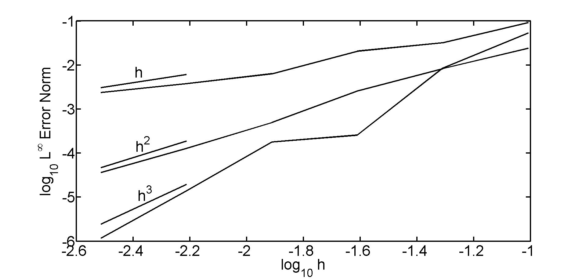
For our tests, we choose a solid region centered at to be . To satisfy the stability restriction, we then take , and slave so that all parameter values are fixed by the number of grid points . For each , with , we then numerically integrate (76) up to a final time of . We repeat the procedure using and derivatives of in constructing the extension and compare the numerical solution to the exact one (i.e. that of the unpenalized problem). Here figure 5 shows the convergence rates for matching different derivatives, while figures 6 and 7 show a typical solution and the corresponding error respectively.


6.2 2D Heat Equation
In the following subsection, we outline the numerical details for a scheme. Here we work with an equispaced, regular grid with points (), and immerse the boundary . The main difference when moving to higher dimensions is how one computes the extension . To illustrate the construction, we refer to figure 8. To build we first compute all appropriate derivatives at each grid point (both on and ). For each grid point within a distance of , we compute as the orthogonal projection of onto and . Using a regular 9 point stencil, we then perform a polynomial interpolation of all required derivatives from the grid points to . Using the interpolated derivatives at , one can then compute the normal derivatives of required in equation (24) to construct at each grid-point inside . Figure 9 illustrates a typical construction of .
Remark 8
For computational efficiency, one can precompute and store the values of as well as the appropriate coefficients required to extrapolate derivatives to the interface .
As an example in , we take the computational domain to be a periodic square with side length . For the penalized domain , we take a circle of radius and center . The physical domain is then . To perform convergence tests, we again use a manufactured solution where . Here we perform a convergence test for the penalty parameter . To compute the convergence rate, we fix and vary , so that discrete numerical errors are smaller than the -dependent error obtained by introducing the penalty term. For different values of , we then integrate the penalty equation for a time and compute the error. Figure 10 shows the error between the penalized equation and the exact heat equation as a function of .


7 Numerical example: 2D incompressible Navier-Stokes
The primary difficulty when transitioning from a penalized heat equation to the penalized incompressible Navier-Stokes equations is the addition of the velocity divergence constraint. Other differences, such as moving from a scalar to a vector equation, or adding a nonlinear convective term do not pose new additional challenges to the penalized equations. Intuitively, the difficulty with the divergence can be outlined as follows. For the penalized heat equation, the active penalty term forces the function to closely track the extension function . When moving to a set of vector equations, the velocity vector will closely track the term inside the penalty region . However, the component-wise construction of will in general be such that . Consequently, to remain consistent, one should not force inside but rather allow to loosely track .
One approach for handling the divergence constraint is to replace with a Pressure Poisson Equation (PPE) [15, 16, 28, 29]. Such an approach can provide a consistent method to compute the pressure and obtain high order schemes. Since a PPE approach requires the additional solution of a Poisson equation with Neumann boundary conditions, we defer the implementation to future work. In our case, we utilize a projection method where we project the velocity divergence to zero inside the fluid domain. We now discretize equations (10)-(11) in time.
7.1 Discretization in time
Here we outline a pseudo-spectral scheme for solving the Navier-Stokes equations. For a second order scheme in , we take a first order discretization in time with a time step restriction of the form outlined in (72). Since the domain is periodic, we can use the Fourier transform to invert the Poisson equation. In the following algorithm we take a regular grid. We also denote the discrete Fourier transform by so that with and .
Algorithm 1
(Navier-Stokes)
- 1.
Given the velocity , compute an intermediate velocity
(77) (78) - 2.
Compute the pressure
(79) For set , while for take
(80) Note that does not appear in the Fourier transform and at no time does one ever compute . The value of is hidden as a consistency condition in setting .
- 3.
Update the velocity
(81)
Note that either Fourier transforms or a second order finite difference scheme can be used when computing the derivatives in algorithm (1).
Since the second derivatives are discontinuous, we compute using finite differences.
In the Poisson equation for the pressure, is only determined up to a constant. To uniquely determine we enforce . Meanwhile the value of is chosen so that the Poisson equation satisfies the standard solvability condition. Namely,
| (82) | |||||
| (83) | |||||
| (84) |
where in the last line we have used the fact that . Here is the volume of the physical domain. The last line also shows that is not nearly as large as since the jump is expected to be small. Finally, we make a remark on the projection of . Inside , we have
| (85) | |||||
| (86) | |||||
| (87) |
where is an appropriate constant. Hence any error in the divergence of is directly controlled by the error in the velocity boundary condition. In particular, for matching derivative, we expect inside . As a result, we can recover a second order scheme, however systematically moving to a higher order method will require an alternative formulation, such as a PPE scheme, for computing the pressure.
Remark 9
In order to guarantee second order spatial accuracy in algorithm (1), should match at least 1 derivative of .
Remark 10
One could also consider solving the Poisson equation (79) with and instead impose an interface condition on the normal pressure gradient:
| (88) |
| (89) |
In the definition (89), is taken as the unit normal directed outward from . Such an approach greatly simplifies the analysis for the behavior of the divergence in the resulting PPE scheme. However, we note that numerically solving (79) with (88) and is harder than simply solving (79)–(82). Furthermore, the equations also allow for a direct solution using pseudo-spectral methods, while the interface problem does not.
To test the order of accuracy of the active penalty method, we again use a manufactured solution of the form and where
| (90) | |||||
| (91) | |||||
| (92) |
Given initial data corresponding to the exact solution, we numerically evolve the velocity and pressure using the pseudo-spectral method outlined in algorithm 1. Here we match 1 derivative of in the construction of and take time steps, with the appropriate restriction, of . Figure 11 shows second order convergence of the velocity field (in ), as well as the pressure and divergence (in ). Meanwhile, the pressure and the divergence converge at one order less in . As an example, figures 13a–13b show the typical error for velocity and pressure while 14a–14b show the velocity divergence. In addition, 15a and 15b show the horizontal velocity field along with the horizontal component of the extension . Note that is again very close to inside .


8 Flow around an impulsively started cylinder
In this section we test our method for the model problem of an impulsively started cylinder [20]. In this case, we solve the following initial value problem where the fluid starts at rest
| (93) |
The impulsively started cylinder is then modeled by a moving mask function with a time dependent set and the appropriate Dirichlet boundary condition. For we have
| (94) | |||
| (95) |
Here is the velocity of the cylinder, and denotes the center and radius of the cylinder.
To simplify the numerical calculation, we perform a Galilean transformation on the coordinates and solve the penalized equations with a stationary mask. The velocity field then solves the equation
| (96) |
with initial data . Here is a stationary mask with , while is the active penalty term with a zero boundary condition .
To compare our results with pre-existing numerical tests, we adopt the following definition of the Reynolds number and time scales from [20]
| RE | (97) | ||||
| (98) |
Using equation (96), we then solve for the velocity field in time, and compute the drag force and lift for the impulsively started cylinder. To compute the force we numerically evaluate the momentum transfer to the fluid
| (99) | |||||
| (100) |
The lift () and drag () coefficients are then evaluated as the non-dimensionalized components of the force
| (101) |
In our numerical tests, we examine the impulsively started cylinder for RE and RE . In both cases, we use , and the appropriate values of to obtain RE. Here figures 16 and 17 show the drag versus time for an impulsively started cylinder with RE and RE respectively. Note that qualitatively the curves match the benchmark results from [20]. In particular, for the RE , the drag coefficient monotonically decays to a value slightly below . Meanwhile, for RE , the drag first drops, followed by a peak at . Here figure 18 shows the early development of vorticity for the impulsive cylinder. We also extend the computation for a much longer time to verify the onset of vortex shedding. Here figure 19 shows the oscillations in the lift coefficient versus time, while 20 shows the vorticity at various times in the evolution. We note that due to the periodicity of the domain, the simulation effectively models an array of cylinders, as opposed to the conventional von Kármán street which arises from flow past one cylinder.


9 Conclusion
In this paper, we outline how to construct high order penalty methods. We do so by first introducing an active penalty term for the heat equation. When we increase the number of matched derivatives, we show that the penalty term improves the analytic convergence rate in terms of the penalty parameter. Secondly, we examine the numerical stability of the active penalty term. We show that it does not introduce additional stiffness into the equations or additional length scales that would need to be resolved. The combination of the high order convergence in the penalty parameter along with the numerical stability then leads to higher order numerical schemes. Lastly, we extend the penalized term from the heat equation to the incompressible Navier-Stokes equations. In particular, we show how to handle the divergence constraint on the velocity field. We also conclude with an application of flow around an impulsively started cylinder for RE and RE . In the case of RE, we demonstrate the onset of a von Kármán street.
Although we have outlined a high order approach, there are still remaining issues that limit the practical feasibility of the method. For instance, at no point do we improve the smoothness of the solution . In fact the second derivatives of remain discontinuous across the curve , although matching more derivatives in the active penalty term may reduce the size of the discontinuity. As a result, Fourier methods still have a slow decay in the Fourier modes thereby limiting the ability to spectrally compute derivatives. In addition, interpolation of high order derivatives in the construction of should be one-sided (i.e. from ) while in practice one would prefer to use points on both sides of . As a result, ongoing research includes improving the global smoothness of while retaining the high order convergence.
10 Acknowledgments
The authors would like to thank Kirill Shmakov and Geneviève Bourgeois for additional preliminary computations not currently presented. The authors have also greatly benefited from conversations with Dmitry Kolomenskiy, Kai Schneider, Ruben Rosales and Tsogtgerel Gantumur. This work was supported by an NSERC Discovery Grant and the NSERC DAS.
References
- [1] P. Angot. A unified fictitious domain model for general embedded boundary conditions. C. R. Math. Acad. Sci. Paris, 341:683–688, 2005.
- [2] P. Angot. A fictitious domain model for the stokes/brinkman problem with jump embedded boundary conditions. C. R. Math. Acad. Sci. Paris, 348:697–702, 2010.
- [3] P. Angot, C.-H. Bruneau, and P. Fabrie. A penalization method to take into account obstacles in incompressible viscous flows. Numer. Math., 81:497–520, 1999.
- [4] P. Angot and J.-P. Caltagirone. New graphical and computational architecture concept for numerical simulation on supercomputers. Proceedings of 2nd World Congress on Computational Mechanics, 1:973–976, 1990.
- [5] E. Arquis and J.-P. Caltagirone. Sur les conditions hydrodynamiques au voisinage d’une interface milieu fluide - milieux poreux: application à la convection naturelle. Comptes Rendus de l’Academie des Science Paris II, 299:1–4, 1984.
- [6] C.-H. Bruneau. Boundary conditions on artificial frontiers for incompressible and compressible navier-stokes equations. M2AN - Mathematical modelling and numerical analysis, 34:303–314, 2000.
- [7] C.-H. Bruneau and P. Fabrie. New efficient boundary conditions for incompressible navier-stokes equations: a well-posedness result. M2AN - Mathematical modelling and numerical analysis, 30:815–840, 1996.
- [8] G. Carbou and P. Fabrie. Boundary layer for a penalization method for viscous incompressible flow, 2003.
- [9] F. Chantalat, C.-H. Bruneau, C. Galusinski, and A. Iollo. Level-set, penalization and cartesian meshes: A paradigm for inverse problems and optimal design. J. Comput. Phys., 228:6291–6315, 2009.
- [10] M. Coquerelle and G.-H. Cottet. A vortex level set method for the two-way coupling of an incompressible fluid with colliding rigid bodies. J. Comput. Phys., 227:9121–9137, 2008.
- [11] R. Fedkiw, T. Aslam, B. Merriman, and S. Osher. A non-oscillatory eulerian approach to interfaces in multimaterial flows (the ghost fluid method). J. Comput. Phys., 152:457–492, 1999.
- [12] G. Folland. Introduction to partial differential equations. Princeton University Press, 2nd edition, 1995.
- [13] F. Gibou, L. Chen, D. Nguyen, and S. Banerjee. A Level set based sharp interface method for the multiphase incompressible Navier-Stokes equations with phase change. J. Comput. Phys., 222:536–555, 2007.
- [14] F. Gibou and R. Fedkiw. A Fourth order accurate discretization for the Laplace and Heat equations on arbitrary domains with applications to the Stefan problem. J. Comput. Phys., 202:577–601, 2005.
- [15] William D. Henshaw. A fourth-order accurate method for the incompressible Navier-Stokes equations on overlapping grids. J. Comput. Phys., 113(1):13–25, July 1994.
- [16] H. Johnston and J-G. Liu. Accurate, stable and efficient navier-stokes solvers based on explicit treatment of the pressure term. J. Comput. Phys., 199:221–259, 2004.
- [17] B. Kadoch, D. Kolomenskiy, P. Angot, and K. Schneider. A volume penalization method for incompressible flows and scalar advection-diffusion with moving obstacles. J. Comput. Phys., 231:4365–4383, 2012.
- [18] K. Khadra, P. Angot, S. Parneix, and J. P. Caltagirone. Fictitious domain approach for numerical modelling of navier-stokes equations. International Journal for Numerical Methods in Fluids, 34:651–684, 2000.
- [19] D. Kolomenskiy and K. Schneider. A fourier spectral method for the navier-stokes equations with volume penalization for moving solid obstacles. J. Comput. Phys., 228:5687–5709, 2009.
- [20] P. Koumoutsakos and A. Leonard. High-resolution simulations of the flow around an impulsively started cylinder using vortex methods. J. Fluid Mech., 296:1–38, 1995.
- [21] B. Le, B. Khoo, and J. Peraire. An immersed interface method for viscous incompressible flows involving rigid and flexible boundaries. J. Comput. Phys., 220:109–138, 2006.
- [22] J. Morales, M. Leroy, W. Bos, and K. Schneider. Simulation of confined magnetohydrodynamic flows using a pseudo-spectral method with volume penalization. J. Comput. Phys. (under review), 2012. hal-00719737, version 1.
- [23] Y. T. Ng, C. Min, and F. Gibou. An efficient fluid-solid coupling algorithm for single-phase flows. J. Comput. Phys., 228:8807–8829, 2009.
- [24] C. Peskin. The immersed boundary method. Acta Numerica, 11:479–517, 2000.
- [25] I. Ramière, P. Angot, and M. Belliard. A general fictitious domain method with immersed jumps and multilevel nested structured meshes. J. Comput. Phys., 225:1347–1387, 2007.
- [26] A. Sarthou, S. Vincent, and J. P. Caltagirone. Consistent velocity-pressure for second-Order -penalty and direct-forcing methods, 2011. hal-00592079, Version 1.
- [27] A. Sarthou, S. Vincent, J. P. Caltagirone, and P. Angot. Eulerian-lagrangian grid coupling and penalty methods for the simulation of multiphase flows interacting with complex objects. International Journal for Numerical Methods in Fluids, 56:1093–1099, 2008.
- [28] D. Shirokoff. I. A pressure Poisson method for the incompressible Navier-Stokes equations : II. Long time behavior of the Klein-Gordon equations. PhD thesis, Massachusetts Institute of Technology, 2011.
- [29] D. Shirokoff and R. R. Rosales. An efficient method for the incompressible Navier-Stokes equations on irregular domains with no-slip boundary conditions, high order up to the boundary. J. Comput. Phys, 230:8619–8646, 2011.
- [30] T. von Kármán. Aerodynamics. McGraw-Hill, 1963.