Feasibility of interference alignment for the
MIMO interference channel
Abstract
We study vector space interference alignment for the MIMO interference channel with no time or frequency diversity, and no symbol extensions. We prove both necessary and sufficient conditions for alignment. In particular, we characterize the feasibility of alignment for the symmetric three-user channel where all users transmit along dimensions, all transmitters have antennas and all receivers have antennas, as well as feasibility of alignment for the fully symmetric () channel with an arbitrary number of users.
An implication of our results is that the total degrees of freedom available in a -user interference channel, using only spatial diversity from the multiple antennas, is at most . This is in sharp contrast to the degrees of freedom shown to be possible by Cadambe and Jafar with arbitrarily large time or frequency diversity.
Moving beyond the question of feasibility, we additionally discuss computation of the number of solutions using Schubert calculus in cases where there are a finite number of solutions.
Index Terms:
interference channel, interference alignment, feasibility of alignment, algebraic geometryI Introduction
Interference is a key bottleneck in wireless communication networks of all types: whenever spectrum is shared between multiple users, each user must deal with undesired signals. Cellular networks in densely populated areas, for example, are severely limited by interference. To address this problem, the research community as well as the wireless communications industry have invested a great deal of effort in trying to develop efficient communication schemes to deal with interference. Nevertheless, the current state-of-the-art systems rely on two basic approaches: either orthogonalizing the communication links across time or frequency, or sharing the same resource while treating other users’ signals as noise. If there are co-located users, these approaches result in a fraction of the total resource being available to each user: performance severely degrades as the number of users increases. Interference alignment is one recent development (among others, such as hierarchical MIMO [3]) that has opened the possibility of significantly better performance in interference-limited communications than traditionally thought possible.
The basic idea of interference alignment is to align, or overlap, multiple interfering signals at each receiver in order to reduce the effective interference. Interference alignment has been used in the index coding literature since the late 90’s, seemingly for the first time by Birk and Kol [4]. For wireless communication, interference alignment was used by Maddah-Ali et al. [5] and made more explicit by Jafar and Shamai [6], both for the multiple-input multiple-output (MIMO) X channel. But the extent of the potential benefit of interference alignment was first observed by Cadambe and Jafar [7] in application to the -user interference channel, when they showed that for time-varying or frequency selective channels with unbounded diversity, total degrees of freedom are achievable using a basic linear precoding scheme. In other words, somewhat amazingly, each user gets the same degrees of freedom as with only two users in the system, independent of the total number of users . The number of degrees of freedom in a system, defined later, is given by the total capacity normalized by the capacity of a single point-to-point link, in the limit of high signal-to-noise ratios (SNR).
The result of Cadambe and Jafar requires unbounded channel diversity, and it is unclear what the implication is for real systems with finite channel diversity. Despite major effort by researchers over the last six or so years, little is known about how diversity affects the ability to align interference. Partial progress in this direction includes [8] for the three-user channel, as well as [9] for single-beam strategies.
Many practical systems are also equipped with multiple antennas and thus have spatial diversity. Multiple antennas are known to greatly increase the degrees of freedom of point-to-point systems. In this paper we focus on how spatial diversity helps to deal with interference by studying interference alignment for the MIMO interference channel. In order to focus on the effect of spatial diversity, we assume there is no time or frequency diversity, i.e., the channel is constant over time and frequency. For technical reasons we additionally restrict attention to strategies making use of a single time-slot (no symbol extensions).
Because [7] uses linear (vector space) precoding, we attempt to simplify matters by restricting to the class of such vector space schemes (defined carefully in Sec. II). Our first results are for the symmetric three user channel. We prove a necessary condition for alignment and give a constructive achievable vector space strategy. These together characterize the feasibility of alignment for signaling dimensions per user in a symmetric system with antennas at the transmitters and antennas at the receivers. The arguments require only basic linear algebra.
Next we generalize to an arbitrary number of users. The arguments make use of tools from algebraic geometry to analyze the bilinear equations arising from the alignment conditions. We first prove a general necessary condition. We subsequently show using Schubert calculus that if and all transmitters use signaling dimensions, then the necessary condition is also sufficient. Schubert calculus is a system for computing the number of solutions to various enumerative problems on algebraic varieties such as Grassmannians. The framework gives an explicit (albeit complicated) combinatorial rule for counting the number of alignment solutions, and in principle allows to check directly if alignment is generically feasible. How to perform this verification is not obvious in general; we argue that the number of solutions is positive in the aforementioned symmetric case.
The rest of the paper is outlined as follows. In Section II we introduce the MIMO interference channel model and formulate the alignment feasibility problem. Section III contains an overview of the main results and comparison with related works. Section IV derives necessary conditions for alignment, and Section V gives sufficient conditions. Finally, Section VI discusses computing the number of alignment solutions as well as how to compute the solutions themselves, and Section VII gives some concluding remarks.
II The MIMO interference channel
The -user MIMO interference channel has transmitters and receivers, with transmitter having antennas and receiver having antennas. For , receiver wishes to obtain a message from the corresponding transmitter . The remaining signals from transmitters are undesired interference. The channel is assumed to be constant over time, and at each time-step the input-output relationship is given by
| (1) |
Here for each user we have and , with the transmitted signal, the received signal, and is additive isotropic white Gaussian noise. The channel matrices are given by for ; for the rest of the paper, we assume that the are generic, meaning that their entries lie outside of an algebraic hypersurface depending only on the parameters , , and . If the entries are randomly chosen from some non-singular probability distribution, this will be true with probability . Additionally, each user obeys an average power constraint, for a block of length .
We restrict the class of coding strategies to (linear) vector space strategies. In this context, degrees-of-freedom has a simple interpretation as the dimensions of the transmit subspaces, described in the next paragraph. However, note that one can more generally define the degrees-of-freedom region in terms of an appropriate high transmit-power limit of the Shannon capacity region normalized by ([5, 7]). In that general framework, it is well-known and straightforward that vector space strategies give a concrete non-optimal achievable strategy with rates
Here is the dimension of transmitter ’s subspace and is the transmit power.
The transmitters encode their data using vector space precoding. Suppose transmitter wishes to transmit a vector of data symbols. These data symbols are modulated on the subspace of dimension , giving the input signal , where is a matrix whose columns give a basis of . This signal is observed by receiver through the channel as . The dimension of the transmit space, , determines the number of data streams, or degrees-of-freedom, available to transmitter . With this restriction to vector space strategies, the output for receiver is given by
| (2) |
The desired signal space at receiver is thus , while the interference space is the span of the undesired subspaces, i.e., .
In the regime of asymptotically high transmit powers, in order that decoding can be accomplished we impose the constraint at each receiver that the desired signal space is complementary to the interference space . Equivalently, receiver must have a subspace (onto which it can project the received signal) with such that
| (3) |
and
| (4) |
Here, means that the two vector spaces are orthogonal with respect to the standard Hermitian form on . Equivalently, if we write and for matrices whose columns form bases for and respectively, then orthogonality means that all entries of the matrix are zero, where denotes the Hermitian transpose.
If each direct channel matrix has generic (or i.i.d. continuously distributed) entries, then the second condition (4) is satisfied assuming for each . This is because the set of channels for which condition (4) is not satisfied obeys a determinant equation and is therefore contained in an algebraic hypersurface (algebraic set of codimension 1). This can be easily justified—see [10] for some brief remarks. Hence we focus on condition (3).
Our goal in this paper is to determine when interference alignment is feasible: given a number of users , numbers of antennas and , and desired transmit subspace dimensions , does there exist a choice of subspaces and with satisfying (3)?
III Main results
As discussed in the previous section, for vector space strategies the alignment problem reduces to finding vector spaces and where is denoted , such that
| (5) |
where the matrix represents the channel between transmitter and receiver . We again emphasize that the are assumed to be generic.
Our goal is to maximize the signal dimensions subject to the constraint that there exist vector spaces satisfying (5). Yetis et al. [11] proposed comparing the number of variables and equations in the system of bilinear equations (5) in order to determine when it has solutions, and justified this using Bernstein’s Theorem in the case that for all . Our first result makes this intuition precise by showing that the feasible solutions are an algebraic variety of the “expected” dimension, when the channel matrices are generic. Thus, we have the following necessary condition for interference alignment:
Theorem 1.
Fix an integer and integers , , and for and suppose the channel matrices are generic. If, for any subset , the quantity
is negative, then there are no feasible strategies. Moreover, if there are feasible strategies, then is the dimension of the variety of solutions.
The constraint on was obtained independently and simultaneously by Razaviyayn et al. [12].
The dimension of the variety of solutions is important, because when multiple strategies are feasible, we may wish to optimize over the feasible strategies according to some other criterion, such as the robustness of the system.
The necessary condition from Theorem 1 is not sufficient. One, almost trivial, requirement for there to even exist vector spaces is that and for each . Similarly, by looking at the total capacity of two transmitters and one receiver, we have the following constraint, which is also implied by combining the information-theoretic arguments of [13] and [14].
Theorem 2.
For any distinct indices , , and , the feasibility of interference alignment requires
Symmetrically, Theorem 2 also holds with the roles of and reversed. Moreover, this result extends to chains of transmitters and receivers longer than three, at least when the transmit and receive dimensions are identical. To do so, rather than three indices , , and from Theorem 2, we use a sequence of indices such that each consecutive triple of indices is distinct. Again, Theorem 3 also applies with and reversed.
Theorem 3.
Fix a non-negative integer and let be a sequence of indices, such that each consecutive triple consists of three distinct indices, i.e., for and for . Also, assume that if then .
Suppose that is the same for all , which we denote , and similarly for . In order for interference alignment to be feasible, we must have:
When is positive, we can rewrite the left-hand side:

The condition on the indices in Theorem 3 is somewhat technical, but the simplest choice is to have cycle through three distinct values. Indeed, in the case of 3 users such a cycle is the only possible sequence and we obtain the following simplification.
Corollary 4.
Suppose that and that and . If interference alignment is feasible, then for any positive integer ,
where for , we define to be , where is the remainder of when divided by .
Of course, Corollary 4 also holds for any reordering of the three users. Moreover, if we assume that the transmit dimensions are all equal to some fixed , then the infeasible parameters correspond to the shaded areas of Figure 1. In fact, as shown by our next theorem, in this symmetric case we have completely characterized the feasible region.
Theorem 5.
Let and without loss of generality, let us assume that . Then interference alignment is feasible if and only if for each ,
| (6) |
Moreover, if, in addition, , then there is a unique solution if and there are solutions if .
The sufficiency of these conditions has also been independently shown by Amir et al. [15], but only in the zero-dimensional case, when . Also independently and simultaneously, Wang et al. [16] have obtained results very similar to Theorem 5. Their necessary condition (which matches the one in Theorem 5) is information-theoretic, and thus, unlike ours, is not limited to linear strategies, constant channels, or no symbol-extensions. The linear achievability result of [16] also matches Theorem 5.
Theorem 5 is constructive in the sense that the solutions can be obtained from basic operations in linear algebra. The reason that the case is easy to analyze is that the constraints (5), which always link a pair of vector space choices, form a cycle in the case of . This cycle allows alignment strategies to be constructed from alignment paths, as was also observed by [16] (and previously in [8] for the three-user interference channel with either time or frequency diversity). When there are more users, we nonetheless have a sufficiency condition in the case when :
Theorem 6.
Suppose that and that and for all users . Then, for generic channel matrices, there is a feasible strategy if and only if .
A very similar theorem was also obtained by Razaviyayn et al. [12] for the case that divides . They found a distinct, but overlapping, set of parameters for which they could characterize feasibility.
Theorem 7 (Theorem 2 in [12]).
Suppose that for all and that and are divisible by for all . Then interference alignment is possible if and only if the quantities from Theorem 1 are non-negative for all subsets .
Rearranging the inequality of Theorem 6, we have that the number of transmit dimensions satisfies .
Corollary 8 (Fully symmetric achievable dof).
The maximum normalized dof is given by
In sharp contrast to the total normalized dof achievable for infinitely many parallel channels in [7], for the MIMO case we see that at most two dof (normalized by the single-user performance of transmit dimensions) are achievable for any number of users and antennas . The difference is due to the structure of the channel matrices: for the MIMO case with full generic matrices condition (3) is difficult to satisfy and (4) is easy, while for the parallel case with diagonal matrices the situation is reversed. We note that this observation was previously made in [11] based on their conjectured necessary condition.
Theorem 6 suggests an engineering interpretation for the performance gain from increasing the number of antennas. Depending on whether or not, there are two different regimes for the performance benefits of increasing : (1) alignment gain or (2) MIMO gain. To illustrate these concepts, suppose that there are users. If , i.e., there is only a single antenna at each node, then no alignment can be done and only one user can communicate on a single dimension, giving 1 total degree of freedom. As the number of antennas increases to and , the number of degrees of freedom becomes and respectively. Because of alignment, the number of users communicating and hence total degrees of freedom increases, which we call alignment gain. The alignment gain has slope . However, after , increasing affords no additional possibilities for interference alignment; the total number of degrees of freedom increases only because more dimensions are available. The MIMO gain has slope , which is the asymptotic coefficient in Corollary 8.
Unlike Theorem 5, the proof of Theorem 6 does not provide a way of computing the solutions. Instead of linear algebra, it uses Schubert calculus to prove the existence of solutions. In fact, in Section VI, we will see that there cannot be a simple, exact description of the symmetric interference alignment problem. Nonetheless, as we will discuss, solutions may be found using numerical algebraic geometry software.
In addition to general algebraic methods of root finding, others have proposed heuristic algorithms, mainly iterative in nature (see [17], [18], [19], [20], and [21]). Some have proofs of convergence, but no performance guarantees are known. Schmidt et al. [21], [22] study a refined version of the single-transmit dimension problem, where for the case that alignment is possible, they attempt to choose a good solution among the many possible solutions. Papailiopoulos and Dimakis [20] relax the problem of maximizing degrees of freedom to that of a constrained rank minimization and propose an iterative algorithm.
In terms of the feasibility problem, González, Beltran, and Santamaría [23] have given a polynomial-time randomized algorithm for determing whether given parameters are feasible. In a slightly different direction, Razaviyayn et al. [19] show that checking the feasibility of alignment for specific system parameters, including the channel matrices, is NP-hard. Note that their result does not contradict that of González et al., since the NP-hardness reduction requires special choices for the channel matrices and does not apply to generic channels.
Finally, we emphasize that our attention has been restricted to vector space interference alignment, where the effect of finite channel diversity can be more easily observed. Interfering signals can also be aligned on the signal scale using lattice codes, which was first proposed in [24] with followup work in [25], [26], and [27]. Recent progress in this direction includes [28], [29], [30], and [31].
IV Necessary conditions
In this section, we prove the necessary conditions for interference alignment, Theorems 1, 3, and 2. The proof of Theorem 1 is by “counting equations,” or, more precisely, by determining the dimension of the relevant algebraic varieties. The proofs of Theorems 3 and 2 use only linear algebra. For background on some of the concepts in algebraic geometry, see the texts by Hartshorne [32] or Shafarevich [33].
In practice, interference alignment requires finding the feasible communications strategies given the fixed channel matrices. However, it will be useful to think of the procedure in reverse: we fix the communication strategy and study the set of channels for which the communication strategy is feasible. As we will see in the proof of Lemma 10, the advantage here is that for a fixed strategy, the constraints on the channel matrices are linear.
To make this approach precise, we will represent the space of strategies as a product of Grassmannians. Recall (for example from [33]) that the Grassmannian is the variety whose points correspond to -dimensional subspaces of an -dimensional vector space . Thus, for each , the transmit subspace corresponds to a point in the Grassmannian, which we also write as , and similarly , where is the complex conjugate of . We choose to parametrize by the complex conjugate because the relation (5) is defined by algebraic equations in the basis of , but not in . The strategy space is thus the product of the Grassmannians,
Likewise, the relevant channel matrices are a tuple of matrices, which we can represent as a point in the product .
In the product , we define the alignment variety to be the subvariety of those ordered pairs such that is a feasible strategy for . The dimensions of and are the sums of the dimensions of their factors, so
| (7) |
and
| (8) |
The dimension of will be computed in Lemma 10, using Theorem 9, which is a rough analogue of the rank-nullity theorem from linear algebra.
Given a map , the fiber of a point is the inverse image of under the map :
A polynomial map is a function whose coordinates are given polynomials. Finally, an irreducible variety is one which cannot be written as the union of two proper, closed subvarieties. The following theorem in algebraic geometry can be found, for example, as Theorem 7 on page 76 of [33].
Theorem 9 (Dimension of fibers).
Let be a polynomial map between irreducible varieties. Suppose that is dominant, i.e., its image is dense in . Let and denote the dimensions of and respectively. Then and:
- 1.
For any and for any component of the fiber the dimension of is at least .
- 2.
There exists a nonempty open subset such that for .
In the proof of Theorem 1, we will apply Theorem 9 twice, for each of the projections from to the factors and . The first of these projections computes the dimension of .
Lemma 10.
is an irreducible variety of dimension
Proof:
We consider the projection from our incidence variety on the space of strategies . For any point , we claim that the fiber is a linear space of dimension
To see this claim, we give local coordinates to each of the subspaces comprising the solution . We write for the th basis element of subspace , where has zeros in the first entries except for a 1 in the th entry, and similarly for (this is without loss of generality). The orthogonality condition can now be written as the condition for each and . Writing this out explicitly, we obtain
Note that this equation is linear in the entries of . There are such linear equations, and each one has a unique variable , so the equations are linearly independent and each equation reduces the dimension by 1. The claim follows from the fact that in total there are equations and we began with dimensions (8).
We have shown that the fibers of are vector spaces, and, in particular, irreducible varieties of constant dimension. Thus, since is an irreducible variety, so is [34, Ex. 14.3]. Moreover, Theorem 9 gives the relation
Since the dimension of is exactly the first summation in the lemma statement, this proves the lemma. ∎
Proof:
We now consider the projection onto the second factor . This map is dominant if and only if the alignment problem is generically feasible. In this case, Theorem 9 tells us that the fiber for a generic has dimension
| (9) |
Using formula (8) for the dimension of and Lemma 10 for the dimension of , we get that (9) is equal to the quantity from the theorem statement. Therefore, by Theorem 9, this quantity must be non-negative if there are to be feasible solutions, in which case is the dimension of the set of solutions to the generic alignment problem.
Now we turn to the necessary conditions for other subsets . Any feasible strategy for the full set of transmitters and receivers, will, in particular be feasible for any subset of trasmitter-reciever pairs. Therefore, a necessary condition for a general set of channel matrices to have a feasible strategy is that the same is true for any subset of the pairs. Since the number is the dimension of the variety of solutions when restricted just to the transmitters and receivers indexed by , then must be non-negative in order to have a feasible strategy. ∎
We now focus on the second necessary condition, Theorem 3, and the closely related Theorem 2. As we mentioned before, Theorem 3 is a generalization of the obvious constraint that for each transmitter, and the generalization is formed by considering transmitters and receivers at the same time. We first handle the case of .
Proof:
We define to be the block matrix:
For generic channel matrices, will have full rank, i.e., rank equal to . We consider the vector space of dimension in . The orthogonality condition (3) implies that . If , then will be injective, and so has dimension . However, orthogonal vector spaces can have at most complementary dimensions, so we have that . On the other hand, if , then the Hermitian transpose is injective, and from the orthogonality relation , we get that . Thus, we conclude that . ∎
A key step in the proof of Theorem 2 was that the matrix had full rank. For , we again show that, under appropriate hypotheses, the analogous matrix has full rank.
Lemma 11.
Let be a sequence as in the statement of Theorem 3, and we assume that and for all . For any define the block matrix to be
| (10) |
For generic channel matrices , the matrix has full rank, .
Proof:
We fix the integer . Define the product of transmit spaces , and similarly let . Note that and have dimensions
First, suppose that . Then Lemma 11 implies that the linear map is injective. By the orthogonality condition (3), we have , and thus
is at most .
Alternatively, if , the Hermitian transpose is an injective linear map . Again, the orthogonality conditions (3) imply that so . This proves the theorem. ∎
V Sufficient conditions
In this section, we give criteria for ensuring the achievability of interference alignment. We have already seen the necessary direction of Theorem 5, and here we prove the sufficient direction, first when , and second when . The former case will also be covered by Theorem 6 dealing with , but we give a specific proof because it is constructive and additionally it allows to compute the number of solutions in the boundary case.
V-A Three users
Proposition 12.
If , and , then alignment is feasible. Moreover, in the case of equality, the number of solutions is exactly for generic channel matrices.
We note that the construction in the following proof has also appeared in [7, Appendix IV].
Proof:
By first restricting our transmit and receive spaces to arbitrary subspaces, we can assume that . Since the channel matrices are square, generically, they are invertible, so we can define the product
Again, generically, this matrix will have linearly independent eigenvectors, and we choose to be the span of any of them. Then we set
These form a feasible strategy, and there are possible strategies. ∎
Before we proceed to the proof in the case when and are distinct, we informally describe the geometry underlying the construction of solutions.
A given vector in the signal space of transmitter is said to initiate an alignment path of length if there exists a sequence of vectors , such that
Here channel indices are interpreted modulo 3. For example, a vector at transmitter 2 initiating an alignment path of length 3 means that there exist vectors and such that and .
The feasible region of Figure 1 is divided up into sub-regions labeled with the maximum length of an alignment path; this number depends on and through the incidence geometry of the images of the channel matrices . We begin by examining sub-region 1, and then look at how things generalize to the other sub-regions.
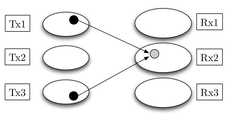
The point of departure is the obvious constraint in order to have a -dimensional subspace of an dimensional vector space. Continuing, assuming , suppose , so lies in sub-region 1 of Figure 1. At receiver one, the images and of the channels from transmitters two and three are in general position and therefore their intersection has dimension ; in other words, alignment is impossible in sub-region 1. Figure 2 shows pictorially that because alignment is not possible here, we have the constraint .
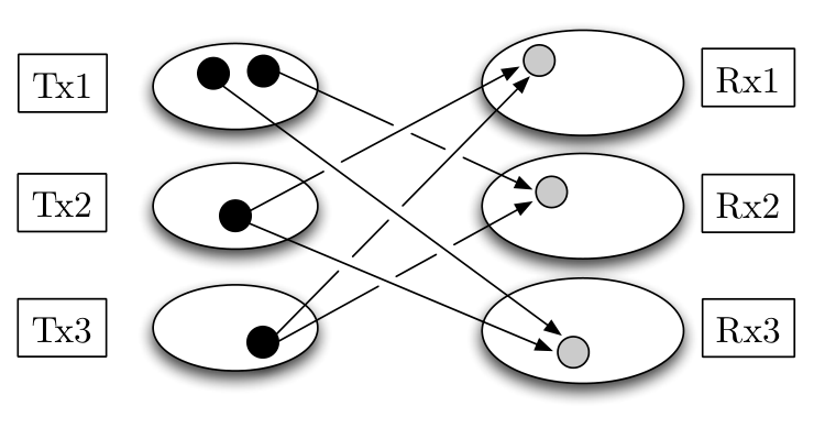
Moving onward to sub-region 2, we have and thus alignment is possible. This means that alignment paths of length 2 are possible (Fig 3), with up to interference dimensions overlapping at each receiver. Thus, the interference space at receiver one occupies at least dimensions, and we have the constraint . However, because , no vector at (say) transmitter three can be simultaneously aligned at both receivers one and two, as indicated in Figure 4. One can also see that no simultaneous alignment is possible by changing perspective to that of a combined receiver one and two. By Lemma 11, the map
| (11) |
from the three transmitters to is injective; analogously to the case in sub-region 1, this is interpreted to mean that no alignment is possible in the combined receive space . Thus, five complementary -dimensional subspaces lie in and we obtain the constraint .
As far as achievability goes, the basic rule-of-thumb is to create alignment paths of maximum length. Thus, in sub-region 2, where alignment is possible, the achievable strategy aligns (as per Fig. 3) as many vectors as possible and the remaining ones (if ) are not aligned. For example, in sub-region 4, alignment paths of length four are used (Fig. 5).
Proposition 13.
If and and (6) holds for each , then alignment is feasible. In the -dimensional case, when , there is a unique solution.
Proof:
We prove achievability by examining two cases: first and second, . Case 1 means that all of the signal space can be obtained from alignment paths of length (up to integer rounding), whereas in case 2 we must use alignment paths of length as well in order to attain the required dimensions.
We first establish case 1. Let be the matrix from (10) for the increasing sequence of indices , where indices are understood modulo . Let be a dimension subspace in the kernel of . Let , and if let be a 1-dimensional subspace in . We define to be the projection of onto its th block of coordinates. The spaces are required in order to accommodate the remainder left when dividing by , and will together contribute dimensions to each signal space . We put
| (15) |
and
| (16) |
where again, the indices in and are understood to be taken modulo three.
If all of ’s constituent subspaces are complementary, then has dimension . We rigorously justify this in Lemma 14. To see that has dimension (at least) , we observe that by subadditivity of dimension,
| (17) |
where if and otherwise. Plugging in the inequality (13) we obtain
Suppose now that we are in case 2: . This means that not all of the signal space can be included in alignment paths of length , so the remainder will be included in alignment paths of length . Let and . As before, denote by the kernel of the matrix , having dimension . Denote by the projection from to the first coordinates. The space is contained in . Let for each be a dimensional subspace in , and let be a 1-dimensional subspace in . Put
| (18) |
and
| (19) |
As before, a naive count suggests that should have dimension , and this will again be justified with Lemma 14.
To see that has dimension at least we again use subadditivity of dimension to get
where is if divides and is otherwise. Letting , we have
Substituting for , the inequality (14) implies that dimV_j≥d+e_2-e_1 . If is one then is strictly positive, so the fact that is an integer implies . ∎
Proof:
We first show that has dimension ; by symmetry of the construction, the dimensions of and will also be .
The subspace is the sum of subspaces , which we claim are independent; suppose to the contrary, that there is some set of linearly dependent vectors , with , and , satisfying . Let be the minimum such value, with all sets of subspaces for being complementary.
Now, by the definition of the subspaces , for each vector there is a sequence of length satisfying . The linear combination thus gives rise to a sequence defined by satisfying
| (20) |
Note that by the minimality assumption of , none of the vectors are zero.
By the definition of , there is a length- sequence of vectors preceding satisfying alignment conditions similar to those in (20); together with and the vectors in (20), this sequence can be extended to a sequence of vectors of total length , none of which are zero. Stacking the first of these vectors produces a nonzero element in the kernel of . However, is full-rank by Lemma 11; the dimension of the kernel is , i.e., the kernel is trivial. This is the desired contradiction.
We now check that has dimension , and again by symmetry, the dimensions of and will also be . Note that if had dimension greater than , we could choose a -dimensional subspace and this would still satisfy the alignment equations (3). But is the orthogonal complement of the sum of subspaces of dimension , so by subadditivity of dimension, we have the lower bound on dimension . ∎
V-B More than three users
We now prove achievability for more than 3 users. We do this under the additional assumption that . Unlike our techniques above, these existence results will not be constructive, a characteristic shared by previous existence proofs in [12] and [1].
In [1], a proof of Theorem 6 was given using dimension theory for algebraic varieties and linear algebra. Here, we give an intersection-theoretic proof, which involves more advanced machinery, but that machinery allows for a more straightforward computation. Moreover, as we will see in Proposition 18, the Schubert calculus framework will also allow us to go beyond the existence of solutions and count the number of solutions when that number is finite.
Our proof will show that the expected number of solutions, as counted by Schubert calculus, is always positive. Schubert calculus is a method for computing the number of solutions to certain enumerative problems. For algebraic varieties, such as the product of Grassmannians that parametrize alignment strategies, there is a commutative ring whose elements correspond to conditions, on the parameters (such as the orthogonality relation (5)), and where the product corresponds to the simultaneous imposition of both conditions. In algebraic geometry, this is known as the Chow ring and in the case of products of Grassmannians, it coincides with the cohomology ring from algebraic topology.
The Chow ring of a Grassmannian has an explicit -basis indexed by partitions. Specifically, the Chow ring of the Grassmannian has a basis corresponding to partitions with at most parts of size at most . Such a partition is a list of integers with , and we write for its size, . The product between two of these basis elements, known as Schubert classes, is given by an intricate combinatorial process known as the Littlewood-Richardson rule.
Thus, to determine whether a given alignment problem is feasible, we proceed in two steps. First, we determine the elements in the Chow ring corresponding to each of the orthogonality conditions (5). Second, we multiply these elements together and the resulting product is non-zero if and only if alignment is feasible. The first step is done by Lemma 17 below. For the second step, the central difficulty is understanding the results of the Littlewood-Richardson rule for products of Schubert classes. In order to establish sufficient conditions in the fully symmetric case, our proof will use carefully chosen terms from each Schubert class, which will be sufficient because the products of the other terms will be non-negative:
Theorem 15.
In the Chow ring of the Grassmannian, the product of two partitions is a non-negative sum of other partitions [35, p. 146, (8)].
For the chosen terms, it will be sufficient to compute their products, not with the general Littlewood-Richardson rule, but by the following simplification:
Proposition 16.
The Schubert classes have the following properties in the Chow ring of the Grassmannian:
- 1.
If and are two partitions with , then the product has a coefficient of in front of the term , where .
- 2.
Suppose that has parts and has parts and that . Then has a coefficient of in front of the term where is formed by concatenating the parts of with the parts of , and then sorting them in decreasing order.
Both parts of this proposition can each be proved from the Pieri rule [35, p. 146, (9)], and in fact they are closely related to each other. Partitions can be depicted as boxes in the upper left corner, such as the depiction of in Figure 6. Such diagrams have an involution by reflecting them along a diagonal so that the conjugate of is the partition . For any partition , we write to denote the conjugate partition. This conjugation corresponds to the isomorphism between and , and it is compatible with the multiplication. The last two items are related by this conjugation operation.
The Chow ring of a product of Grassmannians has a basis indexed by tuples of partitions, one for each Grassmannian. Moreover, the products can be computed factorwise. Formally, the Chow ring of the product of Grassmannians is the tensor product of the Chow rings of the Grassmannians.
We now compute the class in this Chow ring of the variety defined by a single orthogonality condition (5). Our method is similar to the elementary definition of the degree of a projective variety as the number of points in the intersection with a generic linear space of complementary dimension. However, instead of linear spaces, we look at the intersection of Schubert classes of complementary dimension with the set of pairs of vector spaces satisfying (5).
Lemma 17.
The alignment correspondence defined by has class in the Chow ring of . The sum is taken to be over all partitions with at most parts of size at most , and is the partition whose th part has size .
Proof:
We compute the class by intersecting with dual Schubert classes to get a zero-dimensional cycle. In particular, we let and be partitions into at most parts of size at most and respectively, and such that the total size is , which is the dimension of the correspondence.
We first recall the definition of the Schubert variety in associated to a partition and a flag . A flag in is a nested set of vector spaces such that has dimension . The Schubert variety is the closed subvariety of those vector spaces such that
By symmetry, we can assume that is greater than or equal to and thus a vector space uniquely defines an -dimensional subspace in . Likewise, the orthogonal complement is an -dimensional vector space, which together form a flag from dimension through . We can choose a flag of additional vector spaces contained within to get a full flag in , which we denote . Then is in the Schubert variety of if and only if is in the Schubert variety corresponding to and the partition , which we denote . Note that , so and together have total size .
We also fix a flag in , which then defines a Schubert variety in indexed by . We assume that this flag is chosen generically, by which we mean that the intersection is trivial if and has the expected dimension otherwise.
Now we wish to find the points in the intersection of these two Schubert varieties. Passing from to turns the orthogonality condition into containment, so we wish to find pairs satisfying the Schubert conditions
| (21) |
where and . We now let and be indices satisfying . Since has dimension and contains , this means that and must have a non-zero element in common, and thus and must intersect non-trivially. By the generic choice of the flag , this means that the sum of the dimensions of these vector spaces must be at least the dimension of the ambient space, so that we have the inequality . Rearranging, this means that can be at most . Because of their degrees, the only possibility is that for and that for .
Moreover, for fixed partitions and of this type, there is a unique pair of vector spaces satisfying (21). We set to be the vector space generated by the one-dimensional vector spaces for and take to be generated by and .
What we have shown is that the only Schubert classes which occur in the correspondence class are dual to the classes and above, and these occur with coefficient . Since the parts of have size at most , this means that the parts of have size at most , and this is the partition from the lemma statement. Tracing backwards, we see that is , and thus the expression of the correspondence consists of the classes , as in the statement. ∎
Proof:
It will be sufficient to prove that the product of the classes from Lemma 17 over all pairs results in a positive multiple of some Schubert class. Moreover, by Theorem 15, it is sufficient to find one combination of terms from each incidence class whose product is non-zero. We shall exhibit such a combination in two separate cases.
First, we suppose that is odd. From the factor for each incidence correspondence, we choose the term based on the cyclic difference , where is the index of the receiver and is the index of the transmitter. In particular, when this modular difference is between and inclusive, we choose the term where the transmitter partition is . We write to denote the partition consisting of parts of size . By Lemma 17, the term has the empty partition for the receiver’s Grassmannian. When this modular difference is at least , we choose the term where the receiver partition is and the transmitter partition is . Thus, for each Grassmannian, we have the product of copies of . We have assumed that , so this product contains at least one copy the tuple with in each spot.
Suppose now that is even and is also even. We choose the term of each incidence relation as follows (schematically depicted in Fig. 7). The transmitter’s Grassmannian has partition , with the exception that when the transmitter’s index is even and the transmitter’s index is equal to or , modulo , the transmitter has . In either case, the receiver’s partitions are the same. For each receiver, we have the product of copies of and one . The product of with itself has a non-zero coefficient in front of . Then, the product of copies of with has a non-zero coefficient in front of , using our assumption that . At a transmitter with odd index, we are evaluating the product of copies of , yielding a non-zero coefficient in front of . At an even index, it is similar except two of these copies are replaced by , which themselves multiply to , and we get the same result.
Finally, when is even and is odd, the proof is similar, except that since is not an integer, we have to round it up or down each time it is used. In particular, for the factor corresponding to the incidence relation between the th receiver and th transmitter, we use the same partitions above except that we round down in the transmitter’s partition when is even and round up when is odd. Of course, this causes in the receiver’s partition to round in the opposite direction. Overall, for each Grassmannian we have rounded up half the time and down half the time and the product works out as above. ∎
The assumption of a symmetric alignment problem was crucial in being able to choose rectangular Schubert classes in the proof of Theorem 6. The difficulty of generalizing this proof to non-symmetric problems is to find Schubert cycles whose product is provably positive, and unlike the symmetric case, rectangular partitions may not suffice in general.
VI Computing feasible strategies
In this section, we discuss the computation of strategies from particular channel matrices. In the case of , the proofs of sufficiency in Propositions 12 and 13 are effective, in that the feasible strategies can be computed via eigenvectors or the kernel of a matrix, respectively. For , the feasibility problem is not reduced to linear algebra, and the method of Theorem 6 is not constructive, but we can still solve the interference alignment problem using general numerical methods for polynomial equations.
| 1 | 2 | 3 | |
|---|---|---|---|
| 3 | 2 | 6 | 20 |
| 4 | - | 3700 | - |
| 5 | 216 | 388,407,960 | |
| 6 | - | - | |
| 7 | 1,975,560 | ||
| 8 | - | - | |
| 9 | 2,355,206,975,800 | ||
The table shows the number of solutions to the symmetric alignment problem when and either or is even. Missing values could not be computed.
The method used to prove Theorem 6 was to establish a lower bound on the generic number of solutions using Schubert calculus. It was sufficient to find one product of classes which was positive. However, by computing all terms in the product of the incidence relations, we can compute the number of solutions for a general system in small cases:
Proposition 18.
Suppose that either is even or is odd. Then the number of solutions to the symmetric alignment problem is as given in Table I.
Using very different methods, [36, Sec. IV] counted the approximate number of solutions to some interference alignment problems. In the common cases, the two methods agree up to their stated margins of error. In particular, we confirm that for , , and , there are 3700 solutions, which they could only claim with high confidence. In addition, the first two values in Table I for were computed in [22] using Bernstein’s Theorem.
The solution counts given in Proposition 18 are relevant for computing solutions in two different ways. First, a large number of solutions indicate the difficulties in enumerating all solutions or in using an iterative algorithm.
Second, the number of solutions also measures the algebraic complexity of finding a solution, since it is also the degree of the field extension of a solution for random rational parameters. To illustrate this principle, consider the case of Proposition 12, which showed that the solution to the interference alignment problem with and can be found by finding eigenvectors of a matrix. Algebraically, finding an eigenvalue and eigenvector of a generic matrix with rational entries requires solving an irreducible polynomial of degree , and thus the solution lies in a degree extension of the rationals. Finding a second eigenvector requires an extension of degree , and so on, so that the solution lies in a degree extension. A somewhat more refined analysis would show that it lies in a smaller field of degree , but in any case the prime divisors of the degree are less than , and likewise the polynomials that had to be factored had degree less than . The structure of the field extension and its degree reflect the structure of the construction of the solution.
In contrast, Proposition 18 shows us that when, for example, , and , for sufficiently general rational data, the solution lies in an extension of the rationals of degree . Thus, an exact solution must (explicitly or implicitly) entail finding a root of a polynomial of degree , or, worse, some multiple of . It seems unlikely that there is any natural construction for such a polynomial.
Thus, when , we turn to numerical methods, such as PHCpack [37], Bertini [38], and HOM4PS [39], which use homotopy continuation methods to solve arbitrary algebraic equations. Specialized homotopy methods for Schubert problems in a Grassmannian were introduced in [40] and [41]. However, to our knowledge there currently is no implementation of these ideas for Schubert problems in a product of Grassmannians, such as our strategy space.
To represent the unknown vector spaces in the alignment problem, we could use Plücker coordinates. However, computationally, the Plücker coordinates are inefficient and lead to systems with more equations than unknowns, which are more difficult for the numerical solvers. Instead, we choose special coordinates for which our system is square, following [42].
Under our genericity assumptions, we can assume that each is generated by the rows of a matrix with an identity in the leftmost position:
and similarly for . The orthogonality conditions between and can be expressed as bilinear equations in these variables. Note that in this representation, the expected dimension ( in Theorem 1) is the difference between the numbers of variables and the number of equations.
Example 19.
We consider the symmetric alignment problem with , , and . Using Macaulay2 [43], we chose the channel matrices as random matrices with rational entries. Each of the -dimensional vector spaces is given as the span of a vector , and thus there were coordinates. In addition, each of the channel matrices gives one condition, so there were also equations of the form:
We used PHCpack [37] to solve this system and obtained solutions in about a minute and a half on a laptop, thus confirming the value in Table I.
VII Conclusion
This paper makes progress in understanding the role of diversity in aligning interference by focusing on spatial diversity due to multiple antennas. While the performance benefits under the model we have considered are limited, our larger goal has been the introduction of new methods of analysis. The approach we used in [2] and [1] to study vector space strategies for interference alignment has in a short time led to progress in a variety of other channel models and scenarios. For example, under different models in which interaction is allowed between transmitters and receivers, both Annapureddy et al [44] and Geng et al [45] use algebraic techniques to show that substantially better performance may be possible.
[Proof of Lemma 11] In order to prove that has full rank for generic channel matrices, it is sufficient to prove that it does so for one particular set of matrices. This is because having full rank is equivalent to at least one of its maximal minors being non-zero. If this is true for one specialization of the channel matrices, then it will be true for a dense open set. We specialize to the matrices
and
where denotes the identity matrix and the denotes a block of s of size . Note that by our assumptions on the sequence of indices , we have made only one assignment for each matrix in (10).
We will prove that, with these specializations, the block matrix from the statement has full rank by simultaneous induction on , , and . If , then is a matrix, which trivially has full rank. If , then every row vector is a unit vector and all such unit vectors appear in some row, so the matrix has full rank.
Now we suppose that . We permute the rows and columns of as follows. Note that the rows of are arranged into blocks of rows each. We extract the first block in its entirety, followed by the last rows of each of the subsequent blocks. We leave the remaining rows in their induced order, and put extracted rows after them, also in their induced order. We also permute the columns, which are arranged into blocks of size . We take the first block of columns, followed by the last columns of each of the other column blocks, and place these to the right of all the other columns.
If we divide and into blocks by separating off the last rows and columns of each, then we get
where
Therefore, the rearranged matrix has the form
In the lower right, we have a identity matrix of size . We can use this identity matrix, together with elementary column operations to clear the on the left, and with elementary row operations, the s in the upper right. The transformed matrix is in block diagonal form, with an identity matrix in the lower right. In the upper left, the copies of and form our specialized version of with parameters and each decreased by . By the inductive hypothesis, the latter matrix has full rank. Thus, is equivalent to a block diagonal matrix, where one block has full rank, and the other block is the identity, so has full rank.
Acknowledgment
References
- [1] G. Bresler, D. Cartwright, and D. Tse, “Settling the feasibility of interference alignment for the MIMO interference channel: the symmetric square case,” in Information Theory Workshop (ITW), 2011.
- [2] G. Bresler, D. Cartwright, and D. Tse, “Geometry of the 3-user MIMO interference channel,” in Allerton Conference on Communication, Control, and Computing, September 2011. arXiv:1110.5092v1.
- [3] A. Ozgur, O. Lévêque, and D. Tse, “Hierarchical cooperation achieves optimal capacity scaling in ad hoc networks,” IEEE Trans. Inf. Theory, vol. 53, no. 10, pp. 3549–3572, 2007.
- [4] Y. Birk and T. Kol, “Informed-source coding-on-demand (ISCOD) over broadcast channels,” in INFOCOM ’98. Seventeenth Annual Joint Conference of the IEEE Computer and Communications Societies, vol. 3, pp. 1257–1264, 1998.
- [5] M. Maddah-Ali, A. Motahari, and A. Khandani, “Communication over MIMO X channels: Interference alignment, decomposition, and performance analysis,” IEEE Trans. Inf. Theory, vol. 54, pp. 3457–3470, August 2008.
- [6] S. A. Jafar and S. Shamai, “Degrees of freedom region of the MIMO X channel,” IEEE Trans. Inf. Theory, vol. 54, pp. 151–170, January 2008.
- [7] V. Cadambe and S. Jafar, “Interference alignment and degrees of freedom of the -user interference channel,” IEEE Trans. Inf. Theory, vol. 54, pp. 3425–3441, August 2008.
- [8] G. Bresler and D. Tse, “Degrees-of-freedom for the 3-user Gaussian interference channel as a function of channel diversity,” in Allerton Conference on Communication, Control, and Computing, September 2009.
- [9] R. Sun and Z.-Q. Luo, “Two performance-limiting factors for interference alignment: Channel diversity order and the number of data streams per user,” arXiv preprint arXiv:1307.6125, 2013.
- [10] K. Gomadam, V. Cadambe, and S. Jafar, “Approaching the capacity of wireless networks through distributed interference alignment,” in IEEE GLOBECOM, pp. 1 –6, December 2008.
- [11] C. Yetis, T. Gou, S. Jafar, and A. Kayran, “On feasibility of interference alignment in MIMO interference networks,” IEEE Trans. Signal Process., vol. 58, pp. 4771–4782, September 2010.
- [12] M. Razaviyayn, G. Lyubeznik, and Z.-Q. Luo, “On the degrees of freedom achievable through interference alignment in a MIMO interference channel,” IEEE Trans. Signal Process., vol. 60, February 2012.
- [13] T. Gou and S. Jafar, “Degrees of freedom of the user MIMO interference channel,” IEEE Trans. Inf. Theory, vol. 56, pp. 6040 –6057, December 2010.
- [14] S. Jafar and M. Fakhereddin, “Degrees of freedom for the MIMO interference channel,” IEEE Trans. Inf. Theory, vol. 53, pp. 2637 –2642, July 2007.
- [15] M. Amir, A. E. Keyi, and M. Nafie, “A new achievable DoF region for the 3-user symmetric interference channel.” preprint, arXiv:1105.4026v1, May 2011.
- [16] C. Wang, T. Gou, and S. Jafar, “Subspace alignment chains and the degrees of freedom of the three-user MIMO interference channel,” IEEE Trans. Inf. Theory, vol. 50, pp. 2432–2479, May 2014.
- [17] K. Gomadam, V. Cadambe, and S. Jafar, “A distributed numerical approach to interference alignment and applications to wireless interference networks,” IEEE Trans. Inf. Theory, vol. 57, pp. 3309–3322, June 2011.
- [18] S. Peters and R. Heath, “Interference alignment via alternating minimization,” in Acoustics, Speech and Signal Processing, 2009. IEEE International Conference on, pp. 2445–2448, April 2009.
- [19] M. Razaviyayn, M. Sanjabi Boroujeni, and Z.-Q. Luo, “Linear transceiver design for interference alignment: Complexity and computation,” in Signal Processing Advances in Wireless Communications (SPAWC), 2010 IEEE Eleventh International Workshop on, pp. 1–5, June 2010.
- [20] D. S. Papailiopoulos and A. G. Dimakis, “Interference alignment as a rank constrained rank minimization,” in IEEE Trans. Signal Process., vol. 60, pp. 4278–4288, August 2010.
- [21] I. Santamaria, O. Gonzalez, R. Heath, and S. Peters, “Maximum sum-rate interference alignment algorithms for MIMO channels,” in IEEE GLOBECOM, pp. 1–6, December 2010.
- [22] D. A. Schmidt, W. Utschick, and M. L. Honig, “Beamforming techniques for single-beam MIMO interference networks,” in Allerton Conference on Communication, Control, and Computing, pp. 1182–1187, September 2010.
- [23] Ó. González, C. Beltran, and I. Santamaría, “A feasibility test for linear interference alignment in MIMO channels with constant coefficients,” IEEE Trans. Inf. Theory, vol. 60, pp. 1840–1856, March 2014.
- [24] G. Bresler, A. Parekh, and D. Tse, “The approximate capacity of the many-to-one and one-to-many Gaussian interference channels,” IEEE Trans. Inf. Theory, vol. 56, September 2010.
- [25] V. Cadambe, S. Jafar, and S. Shamai, “Interference alignment on the deterministic channel and application to fully connected Gaussian interference networks,” IEEE Trans. Inf. Theory, vol. 55, pp. 269–274, January 2009.
- [26] R. Etkin and E. Ordentlich, “The degrees-of-freedom of the -user Gaussian interference channel is discontinuous at rational channel coefficients,” IEEE Trans. Inf. Theory, vol. 55, pp. 4932–4946, November 2009.
- [27] A. S. Motahari, S. Gharan, M. Maddah-Ali, and A. K. Khandani, “Real interference alignment: Exploiting the potential of single antenna systems.” preprint, arXiv:0908.2282, 2009.
- [28] O. Ordentlich and U. Erez, “Interference alignment at finite SNR for time-invariant channels,” in Information Theory Workshop (ITW), October 2011.
- [29] Y. Wu, S. Shamai, and S. Verdu, “Degrees of freedom of the interference channel: A general formula,” in IEEE International Symposium on Information Theory (ISIT), pp. 1362 –1366, August 2011.
- [30] U. Niesen and M. A. Maddah-Ali, “Interference alignment: From degrees-of-freedom to constant-gap capacity approximations,” in Information Theory Proceedings (ISIT), 2012 IEEE International Symposium on, pp. 2077–2081, IEEE, 2012.
- [31] O. Ordentlich, U. Erez, and B. Nazer, “The approximate sum capacity of the symmetric Gaussian -user interference channel,” in Information Theory Proceedings (ISIT), 2012 IEEE International Symposium on, pp. 2072–2076, IEEE, 2012.
- [32] R. Hartshorne, Algebraic Geometry. Graduate Texts in Mathematics, Springer, 1st ed., 1977.
- [33] I. Shafarevich, Basic Algebraic Geometry. Springer, 2nd ed., 1995.
- [34] D. Eisenbud, Commutative Algebra with a View Toward Algebraic Geometry, vol. 150 of Graduate Texts in Mathematics. Springer, 2004.
- [35] W. Fulton, Young Tableaux, vol. 35 of London Mathematical Society Student Texts. Cambridge University Press, 1997.
- [36] Ó. González and I. Santamaría, “On the number of interference alignment solutions for the -user MIMO channel with constant coefficients.” preprint, arXiv:1301.6196, 2013.
- [37] J. Verschelde, “Polynomial homotopy continuation with PHCpack,” ACM Communcations in Computer Algebra, vol. 44, no. 4, pp. 217–220, 2010.
- [38] D. J. Bates, J. D. Hauenstein, A. J. Sommese, and C. W. Wampler, “Bertini: Software for numerical algebraic geometry.” Available at http://www.nd.edu/~sommese/bertini.
- [39] T. L. Lee, T. Y. Li, and C. H. Tsai, “HOM4PS-2.0: A software package for solving polynomial systems by the polyhedral homotopy continuation method,” Computing, vol. 83, no. 2–3, pp. 109–133, 2008.
- [40] B. Huber, F. Sottile, and B. Sturmfels, “Numerical Schubert calculus,” Journal of Symbolic Computation, vol. 26, no. 6, pp. 767–788, 1998.
- [41] F. Sottile, R. Vakil, and J. Verschelde, “Solving Schubert problems with Littlewood-Richardson homotopies,” in Proceedings of the 2010 International Symposium on Symbolic and Algebraic Computation, pp. 179–186, 2010.
- [42] J. D. Hauenstein, N. Hein, and F. Sottile, “Certifiable numerical computations in Schubert calculus.” preprint, arXiv:1212.3315, 2012.
- [43] D. R. Grayson and M. E. Stillman, “Macaulay2, a software system for research in algebraic geometry.” Available at http://www.math.uiuc.edu/Macaulay2/.
- [44] V. S. Annapureddy, A. El Gamal, and V. V. Veeravalli, “Degrees of freedom of interference channels with CoMP transmission and reception,” IEEE Trans. Inf. Theory, vol. 58, pp. 5740–5760, September 2012.
- [45] Q. Geng, S. Kannan, and P. Viswanath, “Interactive interference alignment,” in Information Theory Proceedings (ISIT), 2013 IEEE International Symposium on, pp. 31–35, IEEE, 2013.