Techniques for Measuring Aerosol Attenuation
using the Central Laser Facility
at the Pierre Auger Observatory
Abstract
The Pierre Auger Observatory in Malargüe, Argentina, is designed to study the properties of ultra-high energy cosmic rays with energies above . It is a hybrid facility that employs a Fluorescence Detector to perform nearly calorimetric measurements of Extensive Air Shower energies. To obtain reliable calorimetric information from the FD, the atmospheric conditions at the observatory need to be continuously monitored during data acquisition. In particular, light attenuation due to aerosols is an important atmospheric correction. The aerosol concentration is highly variable, so that the aerosol attenuation needs to be evaluated hourly. We use light from the Central Laser Facility, located near the center of the observatory site, having an optical signature comparable to that of the highest energy showers detected by the FD. This paper presents two procedures developed to retrieve the aerosol attenuation of fluorescence light from CLF laser shots. Cross checks between the two methods demonstrate that results from both analyses are compatible, and that the uncertainties are well understood. The measurements of the aerosol attenuation provided by the two procedures are currently used at the Pierre Auger Observatory to reconstruct air shower data.
keywords
Ultra-high energy cosmic rays, atmospheric monitoring, aerosolsThe Pierre Auger Collaboration
P. Abreu61,
M. Aglietta49,
M. Ahlers90,
E.J. Ahn78,
I.F.M. Albuquerque15,
I. Allekotte1,
J. Allen82,
P. Allison84,
A. Almela11, 7,
J. Alvarez Castillo54,
J. Alvarez-Muñiz71,
R. Alves Batista16,
M. Ambrosio43,
A. Aminaei55,
L. Anchordoqui91,
S. Andringa61,
T. Antičić22,
C. Aramo43,
F. Arqueros68,
H. Asorey1,
P. Assis61,
J. Aublin28,
M. Ave71,
M. Avenier29,
G. Avila10,
A.M. Badescu64,
K.B. Barber12,
A.F. Barbosa,
R. Bardenet27,
B. Baughman,
J. Bäuml33,
C. Baus35,
J.J. Beatty84,
K.H. Becker32,
A. Bellétoile31,
J.A. Bellido12,
S. BenZvi90,
C. Berat29,
X. Bertou1,
P.L. Biermann36,
P. Billoir28,
F. Blanco68,
M. Blanco28,
C. Bleve32,
H. Blümer35, 33,
M. Boháčová24,
D. Boncioli44,
C. Bonifazi20,
R. Bonino49,
N. Borodai59,
J. Brack76,
I. Brancus62,
P. Brogueira61,
W.C. Brown77,
P. Buchholz39,
A. Bueno70,
L. Buroker91,
R.E. Burton74,
M. Buscemi43,
K.S. Caballero-Mora71, 85,
B. Caccianiga42,
L. Caccianiga28,
L. Caramete36,
R. Caruso45,
A. Castellina49,
G. Cataldi47,
L. Cazon61,
R. Cester46,
S.H. Cheng85,
A. Chiavassa49,
J.A. Chinellato16,
J. Chudoba24,
M. Cilmo43,
R.W. Clay12,
G. Cocciolo47,
R. Colalillo43,
L. Collica42,
M.R. Coluccia47,
R. Conceição61,
F. Contreras9,
H. Cook72,
M.J. Cooper12,
S. Coutu85,
C.E. Covault74,
A. Criss85,
J. Cronin86,
A. Curutiu36,
R. Dallier31, 30,
B. Daniel16,
S. Dasso5, 3,
K. Daumiller33,
B.R. Dawson12,
R.M. de Almeida21,
M. De Domenico45,
S.J. de Jong55, 57,
G. De La Vega8,
W.J.M. de Mello Junior16,
J.R.T. de Mello Neto20,
I. De Mitri47,
V. de Souza14,
K.D. de Vries56,
L. del Peral69,
O. Deligny26,
H. Dembinski33,
N. Dhital81,
C. Di Giulio44,
J.C. Diaz81,
M.L. Díaz Castro13,
P.N. Diep92,
F. Diogo61,
C. Dobrigkeit 16,
W. Docters56,
J.C. D’Olivo54,
P.N. Dong92, 26,
A. Dorofeev76,
J.C. dos Anjos13,
M.T. Dova4,
D. D’Urso43,
J. Ebr24,
R. Engel33,
M. Erdmann37,
C.O. Escobar78, 16,
J. Espadanal61,
A. Etchegoyen7, 11,
P. Facal San Luis86,
H. Falcke55, 58, 57,
K. Fang86,
G. Farrar82,
A.C. Fauth16,
N. Fazzini78,
A.P. Ferguson74,
B. Fick81,
J.M. Figueira7, 33,
A. Filevich7,
A. Filipčič65, 66,
S. Fliescher37,
B.D. Fox87,
C.E. Fracchiolla76,
E.D. Fraenkel56,
O. Fratu64,
U. Fröhlich39,
B. Fuchs35,
R. Gaior28,
R.F. Gamarra7,
S. Gambetta40,
B. García8,
S.T. Garcia Roca71,
D. Garcia-Gamez27,
D. Garcia-Pinto68,
G. Garilli45,
A. Gascon Bravo70,
H. Gemmeke34,
P.L. Ghia28,
M. Giller60,
J. Gitto8,
C. Glaser37,
H. Glass78,
G. Golup1,
F. Gomez Albarracin4,
M. Gómez Berisso1,
P.F. Gómez Vitale10,
P. Gonçalves61,
J.G. Gonzalez35,
B. Gookin76,
A. Gorgi49,
P. Gorham87,
P. Gouffon15,
S. Grebe55, 57,
N. Griffith84,
A.F. Grillo50,
T.D. Grubb12,
Y. Guardincerri3,
F. Guarino43,
G.P. Guedes17,
P. Hansen4,
D. Harari1,
T.A. Harrison12,
J.L. Harton76,
A. Haungs33,
T. Hebbeker37,
D. Heck33,
A.E. Herve12,
G.C. Hill12,
C. Hojvat78,
N. Hollon86,
V.C. Holmes12,
P. Homola59,
J.R. Hörandel55, 57,
P. Horvath25,
M. Hrabovský25, 24,
D. Huber35,
T. Huege33,
A. Insolia45,
S. Jansen55, 57,
C. Jarne4,
S. Jiraskova55,
M. Josebachuili7, 33,
K. Kadija22,
K.H. Kampert32,
P. Karhan23,
P. Kasper78,
I. Katkov35,
B. Kégl27,
B. Keilhauer33,
A. Keivani80,
J.L. Kelley55,
E. Kemp16,
R.M. Kieckhafer81,
H.O. Klages33,
M. Kleifges34,
J. Kleinfeller9, 33,
J. Knapp72,
R. Krause37,
N. Krohm32,
O. Krömer34,
D. Kruppke-Hansen32,
D. Kuempel37,
J.K. Kulbartz38,
N. Kunka34,
G. La Rosa48,
D. LaHurd74,
L. Latronico49,
R. Lauer89,
M. Lauscher37,
P. Lautridou31,
S. Le Coz29,
M.S.A.B. Leão19,
D. Lebrun29,
P. Lebrun78,
M.A. Leigui de Oliveira19,
A. Letessier-Selvon28,
I. Lhenry-Yvon26,
K. Link35,
R. López51,
A. Lopez Agüera71,
K. Louedec29, 27,
J. Lozano Bahilo70,
L. Lu72,
A. Lucero7, 49,
M. Ludwig35,
H. Lyberis20, 26,
M.C. Maccarone48,
C. Macolino28,
M. Malacari12,
S. Maldera49,
J. Maller31,
D. Mandat24,
P. Mantsch78,
A.G. Mariazzi4,
J. Marin9, 49,
V. Marin31,
I.C. Mariş28,
H.R. Marquez Falcon53,
G. Marsella47,
D. Martello47,
L. Martin31, 30,
H. Martinez52,
O. Martínez Bravo51,
D. Martraire26,
J.J. Masías Meza3,
H.J. Mathes33,
J. Matthews80,
J.A.J. Matthews89,
G. Matthiae44,
D. Maurel33,
D. Maurizio13, 46,
E. Mayotte75,
P.O. Mazur78,
G. Medina-Tanco54,
M. Melissas35,
D. Melo7,
E. Menichetti46,
A. Menshikov34,
S. Messina56,
R. Meyhandan87,
S. Mićanović22,
M.I. Micheletti6,
L. Middendorf37,
I.A. Minaya68,
L. Miramonti42,
B. Mitrica62,
L. Molina-Bueno70,
S. Mollerach1,
M. Monasor86,
D. Monnier Ragaigne27,
F. Montanet29,
B. Morales54,
C. Morello49,
J.C. Moreno4,
M. Mostafá76,
C.A. Moura19,
M.A. Muller16,
G. Müller37,
M. Münchmeyer28,
R. Mussa46,
G. Navarra,
J.L. Navarro70,
S. Navas70,
P. Necesal24,
L. Nellen54,
A. Nelles55, 57,
J. Neuser32,
P.T. Nhung92,
M. Niechciol39,
L. Niemietz32,
N. Nierstenhoefer32,
T. Niggemann37,
D. Nitz81,
D. Nosek23,
L. Nožka24,
J. Oehlschläger33,
A. Olinto86,
M. Oliveira61,
M. Ortiz68,
N. Pacheco69,
D. Pakk Selmi-Dei16,
M. Palatka24,
J. Pallotta2,
N. Palmieri35,
G. Parente71,
A. Parra71,
S. Pastor67,
T. Paul91, 83,
M. Pech24,
J. Pȩkala59,
R. Pelayo51, 71,
I.M. Pepe18,
L. Perrone47,
R. Pesce40,
E. Petermann88,
S. Petrera41,
A. Petrolini40,
Y. Petrov76,
C. Pfendner90,
R. Piegaia3,
T. Pierog33,
P. Pieroni3,
M. Pimenta61,
V. Pirronello45,
M. Platino7,
M. Plum37,
V.H. Ponce1,
M. Pontz39,
A. Porcelli33,
P. Privitera86,
M. Prouza24,
E.J. Quel2,
S. Querchfeld32,
J. Rautenberg32,
O. Ravel31,
D. Ravignani7,
B. Revenu31,
J. Ridky24,
S. Riggi48, 71,
M. Risse39,
P. Ristori2,
H. Rivera42,
V. Rizi41,
J. Roberts82,
M.D. Roberts,
W. Rodrigues de Carvalho71,
I. Rodriguez Cabo71,
G. Rodriguez Fernandez44, 71,
J. Rodriguez Martino9,
J. Rodriguez Rojo9,
M.D. Rodríguez-Frías69,
G. Ros69,
J. Rosado68,
T. Rossler25,
M. Roth33,
B. Rouillé-d’Orfeuil86,
E. Roulet1,
A.C. Rovero5,
C. Rühle34,
S.J. Saffi12,
A. Saftoiu62,
F. Salamida26,
H. Salazar51,
F. Salesa Greus76,
G. Salina44,
F. Sánchez7,
C.E. Santo61,
E. Santos61,
E.M. Santos20,
F. Sarazin75,
B. Sarkar32,
R. Sato9,
N. Scharf37,
V. Scherini42,
H. Schieler33,
P. Schiffer38,
A. Schmidt34,
O. Scholten56,
H. Schoorlemmer55, 57,
J. Schovancova24,
P. Schovánek24,
F.G. Schröder33, 7,
J. Schulz55,
D. Schuster75,
S.J. Sciutto4,
M. Scuderi45,
A. Segreto48,
M. Settimo39, 47,
A. Shadkam80,
R.C. Shellard13,
I. Sidelnik1,
G. Sigl38,
O. Sima63,
A. Śmiałkowski60,
R. Šmída33,
G.R. Snow88,
P. Sommers85,
J. Sorokin12,
H. Spinka73, 78,
R. Squartini9,
Y.N. Srivastava83,
S. Stanič66,
J. Stapleton84,
J. Stasielak59,
M. Stephan37,
M. Straub37,
A. Stutz29,
F. Suarez7,
T. Suomijärvi26,
A.D. Supanitsky5,
T. Šuša22,
M.S. Sutherland80,
J. Swain83,
Z. Szadkowski60,
M. Szuba33,
A. Tapia7,
M. Tartare29,
O. Taşcău32,
R. Tcaciuc39,
N.T. Thao92,
D. Thomas76,
J. Tiffenberg3,
C. Timmermans57, 55,
W. Tkaczyk,
C.J. Todero Peixoto14,
G. Toma62,
L. Tomankova33,
B. Tomé61,
A. Tonachini46,
G. Torralba Elipe71,
D. Torres Machado31,
P. Travnicek24,
D.B. Tridapalli15,
E. Trovato45,
M. Tueros71,
R. Ulrich33,
M. Unger33,
M. Urban27,
J.F. Valdés Galicia54,
I. Valiño71,
L. Valore43,
G. van Aar55,
A.M. van den Berg56,
S. van Velzen55,
A. van Vliet38,
E. Varela51,
B. Vargas Cárdenas54,
G. Varner87,
J.R. Vázquez68,
R.A. Vázquez71,
D. Veberič66, 65,
V. Verzi44,
J. Vicha24,
M. Videla8,
L. Villaseñor53,
H. Wahlberg4,
P. Wahrlich12,
O. Wainberg7, 11,
D. Walz37,
A.A. Watson72,
M. Weber34,
K. Weidenhaupt37,
A. Weindl33,
F. Werner33,
S. Westerhoff90,
B.J. Whelan85,
A. Widom83,
G. Wieczorek60,
L. Wiencke75,
B. Wilczyńska,
H. Wilczyński59,
M. Will33,
C. Williams86,
T. Winchen37,
B. Wundheiler7,
T. Yamamoto,
T. Yapici81,
P. Younk79, 39,
G. Yuan80,
A. Yushkov71,
B. Zamorano Garcia70,
E. Zas71,
D. Zavrtanik66, 65,
M. Zavrtanik65, 66,
I. Zaw,
A. Zepeda,
J. Zhou86,
Y. Zhu34,
M. Zimbres Silva32, 16,
M. Ziolkowski39
1 Centro Atómico Bariloche and Instituto Balseiro (CNEA-UNCuyo-CONICET), San
Carlos de Bariloche,
Argentina
2 Centro de Investigaciones en Láseres y Aplicaciones, CITEDEF and CONICET,
Argentina
3 Departamento de Física, FCEyN, Universidad de Buenos Aires y CONICET,
Argentina
4 IFLP, Universidad Nacional de La Plata and CONICET, La Plata,
Argentina
5 Instituto de Astronomía y Física del Espacio (CONICET-UBA), Buenos Aires,
Argentina
6 Instituto de Física de Rosario (IFIR) - CONICET/U.N.R. and Facultad de Ciencias
Bioquímicas y Farmacéuticas U.N.R., Rosario,
Argentina
7 Instituto de Tecnologías en Detección y Astropartículas (CNEA, CONICET, UNSAM),
Buenos Aires,
Argentina
8 National Technological University, Faculty Mendoza (CONICET/CNEA), Mendoza,
Argentina
9 Observatorio Pierre Auger, Malargüe,
Argentina
10 Observatorio Pierre Auger and Comisión Nacional de Energía Atómica, Malargüe,
Argentina
11 Universidad Tecnológica Nacional - Facultad Regional Buenos Aires, Buenos Aires,
Argentina
12 University of Adelaide, Adelaide, S.A.,
Australia
13 Centro Brasileiro de Pesquisas Fisicas, Rio de Janeiro, RJ,
Brazil
14 Universidade de São Paulo, Instituto de Física, São Carlos, SP,
Brazil
15 Universidade de São Paulo, Instituto de Física, São Paulo, SP,
Brazil
16 Universidade Estadual de Campinas, IFGW, Campinas, SP,
Brazil
17 Universidade Estadual de Feira de Santana,
Brazil
18 Universidade Federal da Bahia, Salvador, BA,
Brazil
19 Universidade Federal do ABC, Santo André, SP,
Brazil
20 Universidade Federal do Rio de Janeiro, Instituto de Física, Rio de Janeiro, RJ,
Brazil
21 Universidade Federal Fluminense, EEIMVR, Volta Redonda, RJ,
Brazil
22 Rudjer Bošković Institute, 10000 Zagreb,
Croatia
23 Charles University, Faculty of Mathematics and Physics, Institute of Particle and
Nuclear Physics, Prague,
Czech Republic
24 Institute of Physics of the Academy of Sciences of the Czech Republic, Prague,
Czech Republic
25 Palacky University, RCPTM, Olomouc,
Czech Republic
26 Institut de Physique Nucléaire d’Orsay (IPNO), Université Paris 11, CNRS-IN2P3,
Orsay,
France
27 Laboratoire de l’Accélérateur Linéaire (LAL), Université Paris 11, CNRS-IN2P3,
France
28 Laboratoire de Physique Nucléaire et de Hautes Energies (LPNHE), Universités
Paris 6 et Paris 7, CNRS-IN2P3, Paris,
France
29 Laboratoire de Physique Subatomique et de Cosmologie (LPSC), Université Joseph
Fourier Grenoble, CNRS-IN2P3, Grenoble INP,
France
30 Station de Radioastronomie de Nançay, Observatoire de Paris, CNRS/INSU,
France
31 SUBATECH, École des Mines de Nantes, CNRS-IN2P3, Université de Nantes,
France
32 Bergische Universität Wuppertal, Wuppertal,
Germany
33 Karlsruhe Institute of Technology - Campus North - Institut für Kernphysik, Karlsruhe,
Germany
34 Karlsruhe Institute of Technology - Campus North - Institut für
Prozessdatenverarbeitung und Elektronik, Karlsruhe,
Germany
35 Karlsruhe Institute of Technology - Campus South - Institut für Experimentelle
Kernphysik (IEKP), Karlsruhe,
Germany
36 Max-Planck-Institut für Radioastronomie, Bonn,
Germany
37 RWTH Aachen University, III. Physikalisches Institut A, Aachen,
Germany
38 Universität Hamburg, Hamburg,
Germany
39 Universität Siegen, Siegen,
Germany
40 Dipartimento di Fisica dell’Università and INFN, Genova,
Italy
41 Università dell’Aquila and INFN, L’Aquila,
Italy
42 Università di Milano and Sezione INFN, Milan,
Italy
43 Università di Napoli ”Federico II” and Sezione INFN, Napoli,
Italy
44 Università di Roma II ”Tor Vergata” and Sezione INFN, Roma,
Italy
45 Università di Catania and Sezione INFN, Catania,
Italy
46 Università di Torino and Sezione INFN, Torino,
Italy
47 Dipartimento di Matematica e Fisica ”E. De Giorgi” dell’Università del Salento and
Sezione INFN, Lecce,
Italy
48 Istituto di Astrofisica Spaziale e Fisica Cosmica di Palermo (INAF), Palermo,
Italy
49 Istituto di Fisica dello Spazio Interplanetario (INAF), Università di Torino and
Sezione INFN, Torino,
Italy
50 INFN, Laboratori Nazionali del Gran Sasso, Assergi (L’Aquila),
Italy
51 Benemérita Universidad Autónoma de Puebla, Puebla,
Mexico
52 Centro de Investigación y de Estudios Avanzados del IPN (CINVESTAV), México,
Mexico
53 Universidad Michoacana de San Nicolas de Hidalgo, Morelia, Michoacan,
Mexico
54 Universidad Nacional Autonoma de Mexico, Mexico, D.F.,
Mexico
55 IMAPP, Radboud University Nijmegen,
Netherlands
56 Kernfysisch Versneller Instituut, University of Groningen, Groningen,
Netherlands
57 Nikhef, Science Park, Amsterdam,
Netherlands
58 ASTRON, Dwingeloo,
Netherlands
59 Institute of Nuclear Physics PAN, Krakow,
Poland
60 University of Łódź, Łódź,
Poland
61 LIP and Instituto Superior Técnico, Technical University of Lisbon,
Portugal
62 ’Horia Hulubei’ National Institute for Physics and Nuclear Engineering, Bucharest-
Magurele,
Romania
63 University of Bucharest, Physics Department,
Romania
64 University Politehnica of Bucharest,
Romania
65 J. Stefan Institute, Ljubljana,
Slovenia
66 Laboratory for Astroparticle Physics, University of Nova Gorica,
Slovenia
67 Institut de Física Corpuscular, CSIC-Universitat de València, Valencia,
Spain
68 Universidad Complutense de Madrid, Madrid,
Spain
69 Universidad de Alcalá, Alcalá de Henares (Madrid),
Spain
70 Universidad de Granada and C.A.F.P.E., Granada,
Spain
71 Universidad de Santiago de Compostela,
Spain
72 School of Physics and Astronomy, University of Leeds,
United Kingdom
73 Argonne National Laboratory, Argonne, IL,
USA
74 Case Western Reserve University, Cleveland, OH,
USA
75 Colorado School of Mines, Golden, CO,
USA
76 Colorado State University, Fort Collins, CO,
USA
77 Colorado State University, Pueblo, CO,
USA
78 Fermilab, Batavia, IL,
USA
79 Los Alamos National Laboratory, Los Alamos, NM,
USA
80 Louisiana State University, Baton Rouge, LA,
USA
81 Michigan Technological University, Houghton, MI,
USA
82 New York University, New York, NY,
USA
83 Northeastern University, Boston, MA,
USA
84 Ohio State University, Columbus, OH,
USA
85 Pennsylvania State University, University Park, PA,
USA
86 University of Chicago, Enrico Fermi Institute, Chicago, IL,
USA
87 University of Hawaii, Honolulu, HI,
USA
88 University of Nebraska, Lincoln, NE,
USA
89 University of New Mexico, Albuquerque, NM,
USA
90 University of Wisconsin, Madison, WI,
USA
91 University of Wisconsin, Milwaukee, WI,
USA
92 Institute for Nuclear Science and Technology (INST), Hanoi,
Vietnam
(‡) Deceased
(a) Now at Konan University
(b) Also at the Universidad Autonoma de Chiapas on leave of absence from Cinvestav
(c) Now at University of Maryland
(d) Now at NYU Abu Dhabi
(e) Now at Defence Science and Technology Organisation, Australia
1 Introduction
Direct measurements of primary cosmic rays at ultra-high energies (above ) above the atmosphere are not feasible because of their extremely low flux. The properties of primary particles – energy, mass composition, arrival direction – are deduced from the study of cascades of secondary particles of Extensive Air Showers (EAS), originating from the interaction of cosmic rays with air molecules. The Pierre Auger Observatory [1] in Argentina (mean altitude about 1400 m a.s.l.) combines two well-established techniques: the Surface Detector, used to measure photons and charged particles produced in the shower at ground level; the Fluorescence Detector, used to measure fluorescence light emitted by air molecules excited by secondary particles during shower development. The Fluorescence Detector (FD) [2] consists of 24 telescopes located at four sites around the perimeter of the Surface Detector (SD) array. It is only operated during clear nights with a low illuminated moon fraction. The field of view of a single telescope is 30∘ in azimuth, and 1.5∘ to 30∘ in elevation. Each FD site covers 180∘ in azimuth. The hybrid feature and the large area of 3000 km2 of the observatory enable the study of ultra-high energy cosmic rays with much better precision and much greater statistics than any previous experiment.
The fluorescence technique to detect EAS makes use of the atmosphere as a giant calorimeter whose properties must be continuously monitored to ensure a reliable energy estimate. Atmospheric parameters influence both the production of fluorescence light and its attenuation towards the FD telescopes. The molecular and aerosol scattering processes that contribute to the overall attenuation of light in the atmosphere can be treated separately. In particular, aerosol attenuation of light is the largest time dependent correction applied during air shower reconstruction, as aerosols are subject to significant variations on time scales as little as one hour. If the aerosol attenuation is not taken into account, the shower energy reconstruction is biased by 8 to 25% in the energy range measured by the Pierre Auger Observatory [3]. On average, 20% of all showers have an energy correction larger than 20%, 7% of showers are corrected by more than 30% and 3% of showers are corrected by more than 40%. Dedicated instruments are used to monitor and measure the aerosol parameters of interest: the aerosol extinction coefficient , the normalized differential cross section – or phase function – , and the wavelength dependence of the aerosol scattering, parameterized by the Ångstrom coefficient .
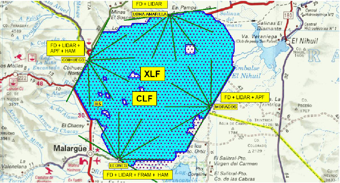
At the Pierre Auger Observatory, molecular and aerosol scattering in the near UV are measured using a collection of dedicated atmospheric monitors [3]. One of these is the Central Laser Facility (CLF) [4] positioned close to the center of the array, as shown in Fig. 1. A newly built second laser station, the eXtreme Laser Facility (XLF), positioned north of the CLF, has been providing an additional test beam since 2009. The two systems produce calibrated 355 nm vertical and inclined laser shots during FD data acquisition. These laser facilities are used as test beams for various applications: to calibrate the pointing direction of telescopes, for the determination of the FD/SD time offset, and for measuring the vertical aerosol optical depth and its differential . An hourly aerosol characterization is provided in the FD field of view with two independent approaches using the same CLF vertical laser events. In the near future, those approaches will be applied to XLF vertical events. The FRAM robotic telescope is used for a passive measurement of the total optical depth of the atmosphere, the horizontal attenuation monitors (HAM) at two of the FD sites are used to characterize the optical properties of the atmosphere close to the ground.
In addition to the CLF and XLF, four monostatic LIDARs [5] and four Infrared Cloud Cameras [6] – one at each FD site – are devoted to cloud and aerosol monitoring. During FD data acquisition, the LIDARs continuously operate outside the FD field of view and detect clouds and aerosols by analyzing the backscatter signal of a 351 nm pulsed laser beam. The cloud cameras use passive measurements of the infrared light and provide a picture of the field of view of every FD telescope every 5 minutes.
To measure the Aerosol Phase Function (APF), a Xenon flash lamp at two of the FD sites fires a set of five shots with a repetition rate of 0.5 Hz once every hour [7]. The shots are fired horizontally across the field of view of five out of the six telescopes in each building. The resulting angular distribution of the signal gives the total scattering phase function as a function of the scattering angle .
In this paper, we will describe the analysis techniques used to estimate aerosol attenuation from CLF laser shots. In Sec. 2 we will review atmospheric attenuation due to aerosols and molecules. In Sec. 3, we will discuss the setup, operation and calibration of the CLF. Sec. 4 contains the description of the two analysis methods used to estimate the aerosol attenuation. Comparisons between the two methods and conclusions follow in Sec. 5 and 6.
2 Atmospheric Attenuation
Molecules in the atmosphere predominantly scatter, rather than absorb, fluorescence photons in the UV range11 1 The most absorbing atmospheric gases in the atmosphere are ozone and NO2. In the 300 to 400 nm range, the contribution of their absorption to the transmission function is negligible [3].. Molecular and aerosol scattering processes can be treated separately. In the following, the term “attenuation” is used to indicate photons that are scattered in such a way that they do not contribute to the light signal recorded by the FD. The molecular and aerosol attenuation processes can be described in terms of atmospheric transmission coefficients and , indicating the fraction of transmitted light intensity as a function of the wavelength and the path length . The amount of fluorescence light recorded at the FD aperture can be expressed in terms of the light intensity at the source as
| (1) |
where H.O. are higher order corrections due to multiple scattering and is the solid angle subtended by the telescope aperture as seen from the light source.
An accurate measurement of the transmission factors during data acquisition is necessary for a reliable reconstruction of the shower and for proper measurements of the physical properties of the primary particle (energy, mass composition, etc). While the molecular transmission factor can be determined analytically once the vertical profiles of atmospheric temperature, pressure, and humidity are known, the aerosol transmission factor depends on the aerosol distribution , where is the aerodynamic radius of the aerosols and is the height above the ground.
The molecular transmission factor is a function of the total wavelength-dependent Rayleigh scattering cross section and of the density profile along the line of sight in atmosphere ,
| (2) |
The Rayleigh scattering cross section is
| (3) |
where is the atmospheric molecular density, measured in molecules per m-3, is the refractive index of the air, and is the King factor that accounts for the anisotropy in the scattering introduced by the non-spherical N2, O2 molecules [8].
The atmospheric density profile along the line of sight is calculated using altitude-dependent temperature and pressure profiles,
| (4) |
where is Avogadro’s number and is the universal gas constant.
Temperature, pressure and humidity vertical profiles of the atmosphere were recorded from August 2002 to December 2010 by performing an intensive campaign of radiosonde measurements above the site of the Pierre Auger Observatory [9]. A set of data was taken about every 20 m during the ascent. The balloons were able to reach altitudes of 25 km a.s.l. on average. Vertical profiles are complemented by temperature, pressure and humidity data from five ground-based weather stations. The measured profiles from these launches have been averaged to form monthly mean profiles (Malargüe Monthly Models) which can be used in the simulation and reconstruction of showers [9, 3]. Currently, the Global Data Assimilation System (GDAS) is used as a source for atmospheric profiles. GDAS combines measurements and forecasts from numerical weather prediction to provide data for the whole globe every three hours. For the location of the Pierre Auger Observatory, reasonable data have been available since June 2005. Comparisons with on-site measurements demonstrate the applicability of the data for air shower analyses [10].
Aerosol scattering can be described by Mie scattering theory. However, it relies on the assumption of spherical scatterers, a condition that is not always fulfilled. Moreover, scattering depends on the nature of the particles. A program to measure the dimensions and nature of aerosols at the Pierre Auger Observatory is in progress and already produced first results, but more study is needed [11]. Therefore, the knowledge of the aerosol transmission factor depends on frequent field measurements of the vertical aerosol optical depth , the integral of the aerosol extinction from the ground to a point at altitude observed at an elevation angle , assuming a horizontally uniform aerosol distribution (cf. Fig. 4),
| (5) |
Hourly measurements of are performed at each FD site using the data collected from the CLF.

Similar to the aerosol transmission factor, the molecular transmission factor for UV light at 355 nm can be calculated using the same geometry,
| (6) |
In Fig. 2, the vertical profile of the molecular optical depth is compared with measured aerosol profiles (Eq. 5) in case of high, average and low aerosols attenuation of light in the air. We define “high” aerosol attenuation when , “average” when and “low” when . Considering an emission point at an altitude of 5 km and a distance on ground of 30 km from the FD, the quoted high, average and low values correspond to transmission factors of , and , respectively. The steps seen in the profiles are due to multiple aerosol layers at different altitudes. For the calculation of the molecular optical depth profile, monthly averaged temperature, pressure, and humidity profiles for the location of the Observatory were used. The 12 resulting profiles were averaged, the fluctuations introduced by the varying atmospheric state variables throughout the year are very small, comparable to the size of the points in Fig 2. On the other hand, the aerosol attenuation can vary between clear and hazy conditions within a few days, making the constant monitoring of the aerosol optical depth necessary.
3 The Central Laser Facility
The Central Laser Facility, described in detail elsewhere [4], generates an atmospheric “test beam”. Briefly, the CLF uses a frequency tripled Nd:YAG laser, control hardware and optics to direct a calibrated pulsed UV beam into the sky. Its wavelength of 355 nm is near the center of the main part of the nitrogen fluorescence spectrum [12]. The spectral purity of the beam delivered to the sky is better than . Light scattered from this beam produces tracks in the FD telescopes. The CLF is located near the middle of the array, nearly equidistant from three out of four of the FD sites, at an altitude of 1416 m above sea level. The distances to the Los Leones (located 1416.2 m above sea level), Los Morados (1416.4 m), Loma Amarilla (1476.7 m) and Coihueco (1712.3 m) FD sites are 26.0 km, 29.6 km, 40 km, and 30.3 km, respectively. In Fig. 3, a picture (left) of the CLF is shown. The CLF is solar-powered and operated remotely.


The laser is mounted on an optical table that also houses most of the other optical components. The arrangement is shown in Fig. 3 (right). Two selectable beam configurations – vertical and steerable – are available. The steering mechanism consists of two mirrors on rotating, orthogonal axes which can direct the beam in any direction above the horizon. The inclined laser shots can be used to calibrate the pointing and time offsets of the fluorescence telescopes. For the aerosol analyses described in this paper, only the vertical beam is used. For this configuration, the beam direction is maintained within 0.04∘ of vertical with full-width beam divergence of less than 0.05∘.
The Nd:YAG laser emits linearly polarized light. To perform the aerosol measurements described in this paper, it is convenient, for reasons of symmetry, to use a vertical beam that has no net polarization. In this case equal amounts of light are scattered in the azimuthal directions of each FD site. Therefore, the optical configuration includes depolarizing elements that randomize the polarization by introducing a varying phase shift across the beam spot. The net polarization of the fixed-direction vertical beam is maintained within 3 of random.
The nominal energy per pulse is 6.5 mJ and the pulse width is 7 ns. Variations in beam energy are tracked to an estimated accuracy of 3. The relative energy of each vertical laser shot is independently measured by a photodiode and a pyroelectric probe. The CLF laser energy is periodically calibrated and optics are cleaned. For each of these periods a new coherent data set is defined and the corresponding period referred to as a CLF epoch. The length of an epoch varies between a few months and one year.
The CLF fires 50 vertical shots at 0.5 Hz repetition rate every 15 minutes during the FD data acquisition. Specific GPS timing is used to distinguish laser from air shower events. The direction, time, and relative energy of each laser pulse is recorded at the CLF and later matched to the corresponding laser event in the FD data.
An upgrade [13] to the CLF is planned for the near future. This upgrade will add a backscatter Raman LIDAR receiver, a robotic calibration system, and replace the current flash lamp pumped laser by a diode pumped laser.
4 CLF Data Analysis

The light scattered out of the CLF laser beam is recorded by the FD (see Fig. 4 for the laser-FD geometry layout). The angles from the beam to the FD for vertical shots are in the range of 90∘ to 120∘. As the differential scattering cross section of aerosol scattering is much smaller than the Rayleigh scattering cross section in this range, the scattering of light is dominated by well-known molecular processes. Laser tracks are recorded by the telescopes in the same format used for air shower measurements. In Fig. 6, a single 7 mJ CLF vertical shot as recorded from the Los Leones FD site is shown. In the left panel of Fig. 6, the corresponding light flux profile for the same event is shown. In Fig. 6, right panel, an average profile of 50 shots is shown.


Laser light is attenuated in the same way as fluorescence light as it propagates towards the FD. Therefore, the analysis of the amount of CLF light that reaches the FD can be used to infer the attenuation due to aerosols. The amount of light scattered out of a 6.5 mJ laser beam by the atmosphere is roughly equivalent to the amount of UV fluorescence light produced by an EAS of eV at a distance to the telescope of about 16 km, as shown in Fig. 7. Also shown is the more attenuated light profile of an almost identical shower at a larger distance.
Besides determining the optical properties of the atmosphere, the identification of clouds is a fundamental task in the analysis of CLF laser shots. Clouds can have a significant impact on shower reconstruction.

In Fig. 8, examples of various hourly profiles affected by different atmospheric conditions are shown. The modulation of the profile is due to the FD camera structure, in which adjacent pixels are complemented by light collectors. A profile measured on a night in which the aerosol attenuation is negligible is shown in panel (a). Profiles measured on nights in which the aerosol attenuation is low, average and high, are respectively shown in panels (b), (c) and (d). As conditions become hazier, the integral photon count decreases. The two bottom profiles (e) and (f) represent cloudy conditions. Clouds appear in CLF light profiles as peaks or holes depending on their position. A cloud positioned between the CLF and the FD can block the transmission of light in its travel from the emission point towards the fluorescence telescopes, appearing as a hole in the profile (e). The cloud could be positioned anywhere between the CLF and the FD site, therefore its altitude cannot be determined unambiguously. A cloud directly above the CLF appears as a peak in the profile, since multiple scattering in the cloud enhances the amount of light scattered towards the FD (f). In this case, it is possible to directly derive the altitude of the cloud from the peak in the photon profile since the laser-detector geometry is known.


Two independent analyses have been developed to provide hourly aerosol characterization in the FD field of view using CLF laser shots from the fixed-direction vertical configuration. To minimize fluctuations, both analyses make use of average light flux profiles normalized to a fixed reference laser energy.
- •
The Data Normalized Analysis is based on the comparison of measured profiles with a reference clear night profile in which the light attenuation is dominated by molecular scattering.
- •
The Laser Simulation Analysis is based on the comparison of measured light flux profiles to simulations generated in various atmospheres in which the aerosol attenuation is described by a parametric model.
Measured profiles are affected by unavoidable systematics related to the FD and laser calibrations. Simulated profiles are also affected by systematics related to the simulation procedure. Using measurements recorded on extremely clear nights where molecular Rayleigh scattering dominates, CLF observations can be properly normalized without the need for absolute photometric calibrations of the FD or laser. We will refer to these nights as reference clear nights. At present multiple scattering effects are not included in the laser simulation code, however the aforementioned normalization includes this effect for Rayleigh scattering, allowing to take it into account in the Laser Simulation Analysis.
4.1 Reference clear nights
In reference clear nights, the attenuation due to aerosols is minimal compared to the uncertainty of total attenuation, the scattering is dominated by the molecular part. In such a clear night, the measured light profiles are larger than profiles affected by aerosol attenuation, indicating maximum photon transmission. Those profiles have shapes that are compatible with a profile simulated under atmospheric conditions in which only molecular scattering of the light is used. Reference clear night profiles are found by comparing measured profiles to simulated average profiles of 50 CLF shots in a purely molecular atmosphere at an energy of 6.5 mJ. Using the Malargüe Monthly Models described in section 2, the procedure is repeated 12 times using the appropriate atmospheric density profiles.
The method chosen for the comparison is the unnormalized Kolmogorov-Smirnov test. This test returns a pseudo-probability22 2 the Kolmogorov-Smirnov test calculates probabilities for histograms containing counts, therefore here the returned value is defined as a pseudo-probability. that the analyzed profile is compatible with the clear one on the basis of shape only, without taking into account the normalization. For each profile, and the ratio between the total number of photons of the measured profile and the simulated clear one is calculated. In each CLF epoch, the search for the reference clear night is performed among profiles having high values of and . A search region is defined by extracting the mean values , and the RMS , of the distribution of each parameter. Both parameters are required to be above their average . Profiles belonging to the search region are grouped by night, and nightly averages for the two parameters are computed and . A list of candidate clear nights with associated pseudo-probabilities and number of profiles is produced. The night with the highest is selected and – if available – at least 4 candidate profiles are averaged to smooth fluctuations. Once identified, the associated is the normalization constant that fixes the energy scale between real and simulated profiles needed in the Laser Simulation Analysis. We estimated the uncertainty introduced by the method chosen to identify the reference clear night by varying the cuts that determine the list of candidate clear nights and the selection criteria that identify the chosen reference night in the list. The normalization constant used to fix the energy scale between real and simulated CLF profiles changes by less than 3.
As a final check to verify that the chosen nights are reference clear nights we analyze the measurement of the aerosol phase function (APF) [7] for that night, measured by the APF monitor (see Sec. 1). The molecular part of the phase function can be calculated analytically from temperature, pressure and humidity at ground provided by weather stations. After subtraction of the molecular phase function, the aerosol phase function remains. In a reference clear night, the total phase function is dominated by the molecular part with almost no contribution from aerosols. Since the APF light source only fires approximately horizontally, this method to find the reference nights is insensitive to clouds, so it can only be used as a verification of reference nights that were found using the procedure described in this section. After verification, the reference night is assumed to be valid for the complete CLF epoch. In Fig. 8, panel (a), an averaged light profile of a reference night is shown.
4.2 Data Normalized Analysis
4.2.1 Building hourly laser profiles and cloud identification
Using the timing of the event, the time bins of the FD data are converted to height at the laser track using the known positions of the FD and CLF. The difference in altitude between telescope and laser station and the curvature of the Earth, which causes a height difference on the order of 50 m, are taken into account. The number of photons is scaled to the number of photons of a 1 mJ laser beam (the normalization energy is an arbitrary choice that has no implications on the measurements). The CLF fires sets of 50 vertical shots every 15 minutes. For each set, an average profile is built.
Clouds are then marked by comparing the photon transmission (see Eq. 5) of the quarter hour profiles to the clear profile bin by bin. A ratio of less than 0.1 indicates a hole in the profile that is caused by a cloud between the laser beam and the FD. A ratio larger than indicates that the laser beam passed through a cloud directly above the CLF causing a spike in the profile. In both cases, the minimum cloud height is set to the height corresponding to the lower edge of the anomaly. Only bins corresponding to heights lower than this cloud height are used for the optical depth analysis. Hours are marked as cloudy only if clouds are found in at least two quarter hour sets, see Fig. 9. If there are no such discontinuities, then is set to the height corresponding to the top of the FD camera field of view.
After is determined, a preliminary full hour profile is made by averaging all the available quarter hour profiles. One or more quarter hour profiles can be missing due to the start or stop of FD data taking, heavy fog, or problems at the CLF. Only one quarter hour profile is required to make a full hour profile. Outlying pixels that triggered randomly during the laser event are rejected and a new full hour profile is calculated. To eliminate outliers in single bins that can cause problems in the optical depth analysis, the quarter hour profiles are subjected to a smoothing procedure by comparing the current profile to the preliminary full hour profile. After multiple iterations of this procedure, the final full hour profile is constructed.
The maximum valid height of the profile is then determined. If there is a hole in the profile of two bins or more due to the rejection of outliers or clouds, is marked at that point. As with , if no such holes exist, then is set to the height corresponding to the top of the FD camera field of view. If is lower than , the minimum cloud height is set to be the maximum valid height. Points above are not usable for data analysis.
4.2.2 Aerosol optical depth calculation
Using the laser-FD viewing geometry shown in Fig. 4, and assuming that the atmosphere is horizontally uniform, it can be shown [14] that the vertical aerosol optical depth is
| (7) |
where is the number of photons from the reference clear profile as a function of height, is the number of photons from the observed hourly profile as a function of height and is defined in Fig. 4. and are the fraction of photons scattered out of the laser beam per unit height by aerosols and air molecules, respectively. is the product of the differential cross section for scattering towards the FD multiplied by the number density of scattering centers. For vertical laser shots , is small compared to because typical aerosols scatter predominately in the forward direction. Thus the second term in Eq. 7 can be neglected to first order and Eq. 7 becomes
| (8) |
With these simplifications, the CLF optical depth measurements depend only on the elevation angle of each laser track segment and the number of photons from the observed track and the reference clear profile. The aerosol optical depth may be calculated directly from Eq. 8.
is calculated for each bin in the hourly profile. The optical depth at the altitude of the telescope is set to zero and is interpolated linearly between the ground and the beginning of corresponding to the bottom of the field of view of the telescope. This calculation provides a first guess of the measured optical depth , assuming that aerosol scattering from the beam does not contribute to the track profile. While this is true for regions of the atmosphere with low aerosol content, is only an approximation of the true if aerosols are present. To overcome this, is differentiated to obtain an estimate of the aerosol extinction in an iterative procedure.
It is possible to find negative values of . They are most likely due to statistical uncertainties in the fit procedure, or can be due to systematic effects. As the laser is far from the FD site, the brightest measured laser light profile, after accounting for relative calibrations of the FD and the laser, occurs during a clear reference night. However, there are uncertainties (see Sec. 4.2.3) in the calibrations that track the FD PMT gains and the CLF laser energy relative to the reference period. Therefore, in some cases it is possible that parts of a laser light profile recorded during a period of interest can slightly exceed the corresponding profile recorded during a reference period. Typically, these artifacts occur during relatively clear conditions when the aerosol concentration is low. The effect could also happen if a localized scattering region, for example a small cloud that was optically too thin to be tagged as a cloud, remained over the laser and scattered more light out of the beam. However, since negative values of are unphysical, they are set to zero. Since the integrated values are renormalized to the measured profile, this procedure does not bias the aerosol profile towards larger values. The remaining values of are numerically integrated to get the fit optical depth . The final values for and can be used for corrections in light transmission during air shower reconstruction.


In Fig. 9, examples of laser and profiles are displayed from an average night and from a cloudy night when the laser pulse passed through a cloud. In the left panels the black traces represent the hourly profiles and the red traces represent the reference clear nights. In the right panels and measurements as a function of height are shown. The black curve is and is overlaid in red. The upper and lower traces correspond to the uncertainties. In the cloudy night, a large amount of light is scattered by a cloud starting from a height of approximately 7000 m. In the bottom right panel, the minimum height at which a cloud was detected is indicated by a vertical blue line.
4.2.3 Determination of Uncertainties
Systematic uncertainties are due to uncertainty in the relative calibration of the FD (), the relative calibration of the laser (), and the relative uncertainty in determination of the reference clear profile (). A conservative estimate for each of these is . These uncertainties are propagated in quadrature for both the hourly profile () and the clear profile (). The systematic uncertainty strongly depends on the height. Thus, the viewing angle from the FD to the laser must be taken into account. The final systematic uncertainty on is calculated by adding and in quadrature, along with the height correction,
| (9) |
Two separate profiles are then generated corresponding to the values of , as shown on the right panels of Fig. 9.
The statistical uncertainty is due to fluctuations in the quarter hour profiles and is considered by dividing the RMS by the mean of all quarter hour profiles at each height. These statistical uncertainties are assigned to each bin of the profiles. These two profiles are then processed through the same slope fit procedure and integration as (see Sec. 4.2.2) to obtain the final upper and lower bounds on .
4.3 Laser Simulation Analysis
4.3.1 Atmospheric Model Description
The atmospheric aerosol model adopted in this analysis is based on the assumption that the aerosol distribution in the atmosphere is horizontally uniform. The aerosol attenuation is described by two parameters, the aerosol horizontal attenuation length and the aerosol scale height . The former describes the light attenuation due to aerosols at ground level, the latter accounts for its dependence on the height. With this parameterization, the expression of the aerosol extinction and the vertical aerosol optical depth are given by
| (10) |
| (11) |
Using Eq. 5, the aerosol transmission factor along the path can be written as
| (12) |
where and are the altitudes above sea level of the first and second observation levels and is the elevation angle of the light path (cf. Fig. 4).
The Planetary Boundary Layer (PBL) is the lower part of the atmosphere directly in contact with the ground, it is variable in height and the aerosol attenuation of light can be assumed as constant. The PBL is neglected in this two parameters approach. In the near future, the mixing layer height will be introduced as a third parameter to take into account the PBL. In the Data Normalized Analysis, is calculated per height bin in the hourly profile, therefore this analysis is sensible to the PBL and takes it into account.
4.3.2 Building quarter-hour CLF profiles and generating a grid of simulations
As described in section 3, the CLF fires 50 vertical shots every 15 minutes. The profile of each individual event of the set is normalized to a reference energy , to compute an average profile equivalent to for each group of 50 shots. In the following, this average light profile will be referred to simply as “profile”. A grid of simulations at the reference energy is generated, fixing the initial number of photons emitted by the simulated vertical laser source. While energy and geometry of the simulated laser event are fixed, the atmospheric conditions, defined by aerosol and air density profiles, are variable and described by means of a two parameters models. The aerosol attenuation profile in the atmosphere, according to the model adopted, is determined setting values for and . For this analysis, the grid is generated by varying from 5 to 150 km in steps of 2.5 km and from 0.5 km to 5 km in steps of 0.25 km, corresponding to a total of 1121 profiles. The air density profiles are provided by the Malargüe Monthly Models, as discussed in Sec 2. Therefore, a total of 13 452 profiles are simulated to reproduce the wide range of possible atmospheric conditions on site. In the left panel of Fig. 10, a measured CLF profile (in blue) is shown together with four out of the 1 121 monthly CLF simulated profiles (in red) used for the comparison procedure. In the right panel, the four aerosol profiles corresponding to the simulated CLF profiles are shown.


The relative energy scale between measured and simulated laser profiles has to be fixed. The amplitude of CLF light profiles from laser shots fired at the same energy depends on the aerosol attenuation in the atmosphere and on absolute FD and CLF calibrations, that are known within 10 and 7, respectively. The ratio of the amplitudes of the simulated clear night to the measured reference clear night as defined in Sec. 4.1 returns the normalization constant that fixes the relative energy scale between measured and simulated laser profiles. Using this normalization procedure, the dependence on FD or CLF absolute calibrations is avoided and only the relative uncertainty (daily fluctuations) of the laser probes (3) and FD calibration constants (3) must be taken into account. This procedure is repeated for each CLF epoch data set. Average measured profiles are scaled by dividing the number of photons in each bin by the normalization constant of the corresponding epoch before measuring the aerosol attenuation.
4.3.3 Optical depth determination and cloud identification
For each quarter hour average profile, the aerosol attenuation is determined obtaining the pair , corresponding to the profile in the simulated grid closest to the analyzed event. The quantification of the difference between measured and simulated profiles and the method to identify the closest simulation are the crucial points of this analysis. After validation tests on simulations of different methods, finally the pair and chosen is the one that minimizes the square difference between measured and simulated profiles computed for each bin, where and are reconstructed photon numbers at the FD aperture in each time bin. In Fig. 11, an average measured profile as seen from Los Leones compared to the simulated chosen profile is shown. The small discrepancy between measured and simulated profiles, corresponding to boundaries between pixels, has no effect on the measurements.

Before the aerosol optical depth is determined, the average profile is checked for integrity and for clouds in the field of view in order to establish the maximum altitude of the corresponding aerosol profile. The procedure for the identification of clouds works on the profile of the difference in photons for each bin between the measured profile under study and the closest simulated profile chosen from the grid. With this choice, the baseline is close to zero and peaks or holes in the difference profile are clearly recognizable. The algorithm developed uses the bin with the highest or lowest signal and the signal-to-noise ratio to establish the presence of a cloud and therefore determines its altitude. The quarter hour information on the minimum cloud layer height needed in the aerosol attenuation characterization is then stored.
If the average profile under study shows any anomaly or if a cloud is detected between the laser track and the FD, it is rejected. If a cloud is detected above the laser track, the profile is truncated at the cloud base height and this lower part of the profile is reanalyzed, since the first search for clouds only identifies the optically thicker cloud layer. If a lower layer of clouds is detected in the truncated profile, or the cloud height is lower than 5500 m a.s.l., the profile is rejected.
If no clouds are detected (either in the whole average profile or in the lower part), the pair , , together with the maximum height of the profile are stored and the procedure is completed. The quarter hour profile is calculated according to Eq. 11 together with the associated statistical and systematic uncertainties. The information is stored, and the quarter hour profiles are averaged to obtain the hourly vertical aerosol optical depth profile and the aerosol extinction profile .
4.3.4 Determination of Uncertainties
Uncertainties on the vertical aerosol optical depth are due to the choice of the reference clear night, to the assumption that a parametric model can be adopted to describe the aerosol attenuation, to the relative uncertainty of nightly FD calibration constants – converting ADC counts to photon numbers – and CLF calibration constants – converting laser probe measurements to laser energy, and to the method used to choose the best matching simulated profile.
To estimate the total uncertainty, the different contributions mentioned above are evaluated and summed in quadrature. The uncertainty on the choice of the reference clear night and the relative FD and CLF calibrations directly affect the light profile, therefore they are summed in quadrature to estimate their total contribution to the uncertainty on the photon profile, which is then propagated to the aerosol profile. The uncertainty introduced by the method used to identify the reference clear night is quoted at 3% as described in Sec. 4.1; the contributions arising from the daily variations on the FD and CLF calibration constants are both quoted at 3% level [4, 2]. Therefore, the total uncertainty of the number of photons in the profile is less than 5.2%. The effect on the aerosol profile of this total uncertainty on the light profile is evaluated by increasing and decreasing the number of photons in the current CLF profile by 5.2% and searching for the corresponding and profiles. At each height, the error bars are given by and .
The contribution due to the parametric description of the aerosol attenuation of light was determined comparing the hourly vertical aerosol optical depth profiles obtained with the Laser Simulation Analysis to the corresponding profiles obtained with the Data Normalized Analysis, which is not using a parametric model for the aerosol attenuation. This comparison for each height shows that aerosol profiles are compatible within 2% at each altitude.
The uncertainty related to the method defined to choose the best matching simulated profile as a function of the altitude is also estimated. As described in Sec. 4.3.3, the parameters and minimize the quantity . The method is repeated a second time in order to find the couple and corresponding to the quantity nearest to . This profile is used to estimate , the uncertainty of the aerosol profile. Therefore, the uncertainty related to the method associated with for each height bin is given by the difference . This uncertainty is negligible with respect to the previous contributions.
The Laser Simulation Analysis extrapolates the aerosol attenuation for each quarter hour CLF profile; then the four measured aerosol profiles are averaged to obtain the hourly information needed for the air shower reconstruction. The same procedure is adopted to obtain the uncertainties related to the hourly aerosol attenuation profile. As a final step, the hourly uncertainty on is propagated to the aerosol extinction .
5 Comparison of the two analyses
The two analyses described in this paper independently produce hourly aerosol profiles. In the Data Normalized Analysis, measured laser light profiles are compared with an averaged light profile of a reference clear night. The Laser Simulation Analysis is a procedure based on the comparison of CLF laser light profiles with those obtained by a grid of simulated profiles in different parameterized atmospheric conditions.
Both analyses have been applied to the whole data set of CLF laser shots. A systematic comparison of the results shows excellent agreement. Since aerosols are concentrated in the lower part of the troposphere, we compare the total vertical aerosol optical depth at 5 km above the FD which includes most of the aerosols. The correlation of (5 km) results of the Data Normalized Analysis and the results of the Laser Simulation Analysis is shown in Fig. 12. The dashed line is a diagonal indicating perfect agreement between the analyses. The solid line is an actual fit to the data. It is compatible with the diagonal. The reliability of the parametric aerosol model adopted and the validity of both methods can be concluded. In high aerosol attenuation conditions, compatible with the presence of a high Planetary Boundary Layer, that the Laser Simulation Analysis does not take into account, the difference between the measured (5 km) is within the quoted systematic uncertainties. Also shown in Fig. 12 are examples for the profiles estimated with the two analyses for conditions with low, average and high aerosol attenuation, respectively.


The high compatibility of the two analyses guarantees a reliable shower reconstruction using aerosol attenuation for the highest possible number of hours. Nearly six years of data have been collected and analyzed (from January 2005 to September 2010). Long term results are shown in the following figures. In the left column of Fig. 13, the time profile of the vertical aerosol optical depth measured 5 km above ground using the Los Leones, Los Morados and Coihueco FD sites is shown. The Loma Amarilla FD site is too far from the CLF to obtain fully reliable results. The XLF is closer and will produce aerosol attenuation measurements for Loma Amarilla in the near future. Values of (5 km) measured during austral winter are systematically lower than in summer.


In the right column of Fig. 13, the (5 km) distribution over six years is shown for aerosol attenuation measurements using the FD sites at Los Leones, Los Morados and Coihueco. More than 5000 hours of aerosol profiles have been measured with each FD. The average (5 km) measured with different FD sites are compatible. The average value measured above Coihueco is slightly smaller due to the higher position ( 300 m) of the Coihueco FD site with respect to Los Leones and Los Morados.
6 Conclusions
Aerosols cause the largest time-varying corrections applied during the reconstruction of extensive air showers measured with the fluorescence technique. They are highly variable on a time scale of one hour. Neglecting the aerosol attenuation leads to a bias in the energy reconstruction of air showers by 8 to 25% in the energy range measured by the Pierre Auger Observatory. This includes a tail of 7% of all showers with an energy correction larger than 30%.
To determine the vertical aerosol optical depth profiles for the Pierre Auger Observatory, vertical laser shots from a Central Laser Facility in the center of the SD array are analyzed. The Central Laser Facility fires 50 vertical shots every 15 minutes during the FD data acquisition, covering the whole FD data taking period. Two methods were developed to analyze the CLF laser shots. The Data Normalized method compares the measured laser light profile to a reference clear night, the Laser Simulation method compares the measured profile with a set of simulated profiles. In addition, the minimum cloud heights over the central part of the array are extracted from the laser data. The two methods are compared and a very good agreement was found. Nearly six years of data have been analyzed with both methods (from January 2005 to September 2010). In air shower reconstructions, mainly the results of the Data Normalized method are used. The data from the Laser Simulation method is used to fill holes in the data set where the Data Normalized method is not able to produce a result.
Acknowledgments
The successful installation, commissioning, and operation of the Pierre Auger Observatory including the Central Laser Facility would not have been possible without the strong commitment and effort from the technical and administrative staff in Malargüe.
We are very grateful to the following agencies and organizations for financial support: Comisión Nacional de Energía Atómica, Fundación Antorchas, Gobierno De La Provincia de Mendoza, Municipalidad de Malargüe, NDM Holdings and Valle Las Leñas, in gratitude for their continuing cooperation over land access, Argentina; the Australian Research Council; Conselho Nacional de Desenvolvimento Científico e Tecnológico (CNPq), Financiadora de Estudos e Projetos (FINEP), Fundação de Amparo à Pesquisa do Estado de Rio de Janeiro (FAPERJ), Fundação de Amparo à Pesquisa do Estado de São Paulo (FAPESP), Ministério de Ciência e Tecnologia (MCT), Brazil; AVCR AV0Z10100502 and AV0Z10100522, GAAV KJB100100904, MSMT-CR LA08016, LC527, 1M06002, MEB111003, and MSM0021620859, Czech Republic; Centre de Calcul IN2P3/CNRS, Centre National de la Recherche Scientifique (CNRS), Conseil Régional Ile-de-France, Département Physique Nucléaire et Corpusculaire (PNC-IN2P3/CNRS), Département Sciences de l’Univers (SDU-INSU/CNRS), France; Bundesministerium für Bildung und Forschung (BMBF), Deutsche Forschungsgemeinschaft (DFG), Finanzministerium Baden-Württemberg, Helmholtz-Gemeinschaft Deutscher Forschungszentren (HGF), Ministerium für Wissenschaft und Forschung, Nordrhein-Westfalen, Ministerium für Wissenschaft, Forschung und Kunst, Baden-Württemberg, Germany; Istituto Nazionale di Fisica Nucleare (INFN), Ministero dell’Istruzione, dell’Università e della Ricerca (MIUR), Italy; Consejo Nacional de Ciencia y Tecnología (CONACYT), Mexico; Ministerie van Onderwijs, Cultuur en Wetenschap, Nederlandse Organisatie voor Wetenschappelijk Onderzoek (NWO), Stichting voor Fundamenteel Onderzoek der Materie (FOM), Netherlands; Ministry of Science and Higher Education, Grant Nos. N N202 200239 and N N202 207238, Poland; Fundação para a Ciência e a Tecnologia, Portugal; Ministry for Higher Education, Science, and Technology, Slovenian Research Agency, Slovenia; Comunidad de Madrid, Consejería de Educación de la Comunidad de Castilla La Mancha, FEDER funds, Ministerio de Ciencia e Innovación and Consolider-Ingenio 2010 (CPAN), Xunta de Galicia, Spain; Science and Technology Facilities Council, United Kingdom; Department of Energy, Contract Nos. DE-AC02-07CH11359, DE-FR02-04ER41300, National Science Foundation, Grant Nos. 0450696, 0855680, The Grainger Foundation USA; NAFOSTED, Vietnam; ALFA-EC / HELEN, European Union 6th Framework Program, Grant No. MEIF-CT-2005-025057, European Union 7th Framework Program, Grant No. PIEF-GA-2008-220240, and UNESCO.
References
- [1] The Pierre Auger Collaboration, J. Abraham et al., Properties and performance of the prototype instrument for the Pierre Auger Observatory, Nucl. Instr. Meth. A523 (2004) 50–95.
- [2] The Pierre Auger Collaboration, J. Abraham et al., The Fluorescence Detector of the Pierre Auger Observatory, Nucl. Instr. Meth. A620 (2010) 227–251, [arXiv:0907.4282].
- [3] The Pierre Auger Collaboration, J. Abraham et al., A Study of the Effect of Molecular and Aerosol Conditions in the Atmosphere on Air Fluorescence Measurements at the Pierre Auger Observatory, Astropart. Phys. 33 (2010) 108–129, [arXiv:1002.0366].
- [4] B. Fick et al., The Central Laser Facility at the Pierre Auger Observatory, JINST 1 (2006) P11003, [astro-ph/0507334].
- [5] S. Y. BenZvi et al., The Lidar System of the Pierre Auger Observatory, Nucl. Instr. Meth. A574 (2007) 171–184, [astro-ph/0609063].
- [6] K. Louedec for the Pierre Auger Collaboration, Atmospheric Monitoring at the Pierre Auger Observatory – Status and Update, in Proc. 32nd ICRC, vol. 2, (Beijing, China), pp. 63–66, 2011, [arXiv:1107.4806].
- [7] S. Y. BenZvi et al., Measurement of the aerosol phase function at the Pierre Auger Observatory, Astropart. Phys. 28 (2007) 312–320, [arXiv:0704.0303].
- [8] L. V. King, On the complex anisotropic molecule in relation to the dispersion and scattering of light, Proc. R. Soc. London Ser. A 104 (1923) 333–357.
- [9] B. Keilhauer and M. Will, Description of Atmospheric Conditions at the Pierre Auger Observatory Using Meteorological Measurements and Models, Eur. Phys. J. Plus 127 (2012) 96–105, [arXiv:1208.5417].
- [10] The Pierre Auger Collaboration, P. Abreu et al., Data from the Global Data Assimilation System (GDAS) for the Pierre Auger Observatory, Astropart. Phys. 35 (2012) 591–607, [arXiv:1201.2276].
- [11] M. I. Micheletti et al., Elemental analysis of aerosols collected at the Pierre Auger Cosmic Ray Observatory with PIXE technique complemented with SEM/EDX, Nucl. Instr. Meth. B288 (2012) 10–17.
- [12] The AIRFLY Collaboration, M. Ave et al., Spectrally resolved pressure dependence measurements of air fluorescence emission with AIRFLY, Nucl. Inst. Meth. A597 (2008) 41–45.
- [13] L. Wiencke et al. for the Pierre Auger Collaboration, Atmospheric “Super Test Beam” for the Pierre Auger Observatory, in Proc. 32nd ICRC, vol. 3, (Beijing, China), pp. 141–144, 2011, [arXiv:1107.4806].
- [14] The High Resolution Fly’s Eye Collaboration (HiRes), R. U. Abbasi et al., Techniques for measuring atmospheric aerosols at the High Resolution Fly’s Eye experiment, Astropart. Phys. 25 (2006) 74–83, [astro-ph/0512423].