Justification of Leading Order Quasicontinuum Approximations of Strongly Nonlinear Lattices

Abstract.

We consider the leading order quasicontinuum limits of a one-dimensional granular medium governed by the Hertz contact law under precompression. The approximate model which is derived in this limit is justified by establishing asymptotic bounds for the error with the help of energy estimates. The continuum model predicts the development of shock waves, which are also studied in the full system with the aid of numerical simulations. We also show that existing results concerning the Nonlinear Schrödinger (NLS) and Korteweg de-Vries (KdV) approximation of FPU models apply directly to a precompressed granular medium in the weakly nonlinear regime.

Key words and phrases:

quasicontinuum approximation, error estimates, granular crystals, strongly nonlinear, shocks

1991 Mathematics Subject Classification

Primary: 35Q70, 34K07; Secondary: 35L67 .

Christoper Chong and P.G. Kevrekidis

Department of Mathematics and Statistics

University of Massachusetts

Amherst, MA 01003-9305, USA

Guido Schneider

Institut für Analysis, Dynamik und Modellierung

Universität Stuttgart

Pfaffenwaldring 57, 70569 Stuttgart, Germany.

1. Introduction

We consider a one-dimensional granular medium which is governed by the Hertz law. Denote $q_{n}$ the relative displacement from equilibrium of the $n$ -th particle. Then the renormalized equations of motion describing the $q_{n}$ ’s have the form [12],

\ddot{q}_{n}=W^{\prime}(q_{n-1}-q_{n})-W^{\prime}(q_{n}-q_{n+1}),\qquad(n\in\mathbb{Z}),

(1)

where

W^{\prime}(u)=\left[\delta_{0}+u\right]_{+}^{p},\qquad[u]_{+}=u\,\Theta(u)=\mathrm{max}(0,u)

(2)

where $\Theta$ is the Heaviside function and $\delta_{0}$ is the static load (precompression) applied to the chain at all times. There is a double nonlinearity stemming from this system due to the lack of tensile strength (resulting in an asymmetric potential function $W$ ) and the nonlinear coupling. For spherical particles we have $p=3/2$ , which corresponds to the classical Hertz contact law.

It will be convenient to work with the difference $u_{n}=q_{n-1}-q_{n}$ , i.e. the strain, which satisfies

\ddot{u}_{n}=W^{\prime}(u_{n+1})-2W^{\prime}(u_{n})+W^{\prime}(u_{n-1}),\qquad(n\in\mathbb{Z}).

(3)

With the long wave ansatz

u_{n}(t)=A(X,T),\qquad X=\varepsilon n,\quad T=\varepsilon t

where $X,T,A(X,T)\in\mathbb{R}$ and $\varepsilon\ll 1$ is a small perturbation parameter, one can derive the leading order continuum model approximation to the discrete dynamics

\partial^{2}_{T}A=\partial^{2}_{X}((\delta_{0}+A)^{p}).

(4)

The main result of the present paper is the following approximation theorem.

Theorem 1.1.

Fix $\delta_{0}>0$ and let $p\in\mathbb{R}^{+}$ and let $A\in C\left(\left[0,T_{0}\right],H^{4}\right)$ with

\sup_{T\in\left[0,T_{0}\right]}\sup_{X\in\mathbb{R}}\left|A(X,T)\right|\leq\delta_{0}/2\qquad\textrm{and}\qquad\sup_{T\in\left[0,T_{0}\right]}\|A(\cdot,T)\|_{H^{4}}\leq C_{1}

be a solution of (4). Then for $C_{1}>0$ sufficiently small there exists $C,\varepsilon_{0}>0$ such that for all $\varepsilon\in(0,\varepsilon_{0})$ there are solutions $(u_{n}(t))_{n\in\mathbb{Z}}$ of (3) satisfying

\sup_{t\in[0,T_{0}/\varepsilon]}\sup_{n\in\mathbb{Z}}\left|u_{n}(t)-A(\varepsilon n,\varepsilon t)\right|<C\varepsilon^{3/2}.

In the weakly nonlinear case, i.e. if the precompression is much greater than the amplitude of the solution, then the Nonlinear Schrödinger (NLS) and Korteweg de-Vries (KdV) equations can be derived as continuum models for solutions that have amplitude of order $\mathcal{O}(\varepsilon)$ and $\mathcal{O}(\varepsilon^{2})$ respectively, see Section 8. For solutions of order $\mathcal{O}(1)$ (i.e. solutions with amplitude that are on the same order as the precompression) model (4) is relevant. In order to establish local existence and uniqueness of the continuum model and to handle the nonlinearity in Fourier space, we will expand the nonlinearity as a series. Since the amplitude is $\mathcal{O}(1)$ we cannot truncate this series (which is done when deriving the NLS and KdV equations). Therefore, we require that the precompression is of the same order as the amplitude (but not greater). It is unclear if this is only a technical assumption or if it is really necessary for having the approximation property. It will be the subject of future research to explore whether or not the assumptions of Theorem 1.1 can be relaxed, and if so, how the continuum model (4) needs to be modified.

If one does not ignore higher order terms in the derivation (see next section), then one arrives at the following $\mathcal{O}(1)$ continuum model for the strain in the purely nonlinear case (if $\delta_{0}=0$ )

\partial^{2}_{T}A=\partial^{2}_{X}(A^{p})+\frac{\epsilon^{2}}{12}\partial_{x}^{4}(A^{p})

(5)

which is the equation derived in [1] (where the small parameter $\varepsilon$ is formally set to unity). From a physical standpoint, the reason for doing so is understandable, as the higher order term in the model affords the existence of exact localized traveling wave solutions (which do not exist in the continuum model (4)). An alternative approach towards such a (higher order) quasi-continuum model is the one spearheaded in the earlier work of [12], where one does a similar formal Taylor-expansion based calculation at the displacement level and then differentiates with respect to $x$ to derive the effective long-wavelength equation for the strains $r=q_{x}$ . Remarkably, it should be pointed out, as indicated in [1], that these two procedures (reverting to strain variables and Taylor expanding to go to long wavelengths) do not commute, a feature which poses a mathematical challenge in its own right (about their respective validity). It should be noted that from a visual inspection the solitary wave profiles predicted by (5) (and the corresponding ones of [12]) compare quite well with the “numerically exact” traveling wave solution of the granular crystal model (3) [1]. Nevertheless, without an approximation theorem, it is not clear to what level/extent these kinds of approximations can be used. For example, for the initial value problem (and not just for very special solutions, such as the exact traveling wave ones), there are several nontrivial concerns about models such as those of [1, 12] in connection to their local uniqueness and existence properties and the fact the solutions will depend on the small parameter $\epsilon$ (hence it is unclear what, if any, influence the $\mathcal{O}(\epsilon)$ terms have on the dynamics on the $O(1)$ time scale w.r.t. $T$ ). Thus, in terms of providing rigorous error estimates for the initial value problem, model (4) is more appropriate, at least as a starting point or a leading order approximation. Although Eq. (4) fails to describe exact traveling solitary waves (and hence the proper, controllable generalization to higher order so as to capture this important trait is, from a rigorous perspective, an open problem), the model does well in other regards, such as in the description of shock wave formation. This, and other properties of (4) are described in Sections 4 and 7.

Notation. Throughout this paper many possibly different constants are denoted with the same symbol $C$ if they can be chosen independently of the small perturbation parameter $0<\varepsilon\ll 1$ .

2. Fourier transform as fundamental tool

The Fourier transform is the major tool in the proof of the approximation result. In this section we recall some basic facts and establish notation conventions.

Since the solutions $u$ of (3) live on $\mathbb{Z}$ we need the Fourier transform on $\mathbb{Z}$ leading to periodic functions in Fourier space.

Fourier transform on $\mathbb{Z}$ :

System (3) can be transferred into Fourier space by

\hat{u}(k,t)=\mathcal{F}(u)(k,t)=\frac{1}{2\pi}\sum_{n\in\mathbb{Z}}u_{n}(t)e^{-ikn}.

(6)

The inverse of $\mathcal{F}$ is given by

u_{n}(t)=(\mathcal{F}^{-1}\hat{u})_{n}(t)=\int_{-\pi}^{\pi}\hat{u}(k,t)e^{ikn}dk.

(7)

For every $s\geq 0$ the Fourier transform $\mathcal{F}$ is continuous from

\ell^{2}_{s}=\{u:\mathbb{Z}\to\mathbb{R}\ |\ \|u(\cdot)\|_{\ell^{2}_{s}}<\infty\}

into

	$\displaystyle H^{s}_{\rm per}(\mathbb{R},\mathbb{C})=$	$\displaystyle\{\hat{u}:\mathbb{R}\to\mathbb{C}\ \|\ \hat{u}(\cdot)\ \mathrm{is}\ s\ \mathrm{times\ weakly\ differentiable},$
		$\displaystyle\quad\\|\hat{u}(\cdot)\\|_{H^{s}_{\rm per}}<\infty,\ \hat{u}(k)=\hat{u}(k+2\pi)\}$

where

\|u(\cdot,t)\|_{\ell^{2}_{s}}^{2}=\sum_{n\in\mathbb{Z}}(|u_{n}(t)|^{2}(1+n^{2})^{s})\quad{\rm and}\quad\|\hat{u}(\cdot,t)\|_{H^{s}_{\rm per}}^{2}=\sum_{m=0}^{s}(\int_{-\pi}^{\pi}|\partial_{k}^{m}\hat{u}(k,t)|^{2}dk).

The inverse Fourier transform $\mathcal{F}^{-1}$ is continuous from $H^{s}_{\rm per}$ into $\ell^{2}_{s}$ and from $L^{1}_{\rm per}$ into $\ell^{\infty}$ where

\|\hat{u}(\cdot,t)\|_{L^{1}_{\rm per}}=\int_{-\pi}^{\pi}|\hat{u}(k,t)|dk\qquad{\rm and}\qquad\|u(\cdot,t)\|_{\ell^{\infty}}=\sup_{n\in\mathbb{Z}}|u_{n}(t)|.

Fourier transform on $\mathbb{R}$ :

Beside the Fourier transform on $\mathbb{Z}$ we need the Fourier transform on the real line in order to handle the continuum model which lives on the real line. We set

\hat{u}(k,t)=\mathcal{F}(u)(k,t)=\frac{1}{2\pi}\int_{-\infty}^{\infty}u(x,t)e^{-ikx}dx.

(8)

The inverse is given by

u(x,t)=\mathcal{F}^{-1}(\hat{u})(x,t)=\int_{-\infty}^{\infty}\hat{u}(k,t)e^{ikx}dk.

(9)

For every $s\geq 0$ the Fourier transform $\mathcal{F}$ is continuous from

L^{2}_{s}=\{u:\mathbb{R}\to\mathbb{C}\ |\ \|u(\cdot)\|_{L^{2}_{s}}<\infty\}

into

\displaystyle H^{s}(\mathbb{R},\mathbb{C})

\displaystyle=

\displaystyle\{\hat{u}:\mathbb{R}\to\mathbb{C}\ |\ \hat{u}(\cdot)\ \mathrm{is}\ s\ \mathrm{times\ weakly\ differentiable},\ \|\hat{u}(\cdot)\|_{H^{s}}<\infty\ \}

where

\|u(\cdot,t)\|_{L^{2}_{s}}^{2}=\int_{-\infty}^{\infty}(|u(x,t)|^{2}(1+x^{2})^{s})dx\quad{\rm and}\quad\|\hat{u}(\cdot,t)\|_{H^{s}}^{2}=\sum_{m=0}^{s}(\int_{-\infty}^{\infty}|\partial_{k}^{m}\hat{u}(k,t)|^{2}dk).

The Fourier transform $\mathcal{F}$ and its inverse $\mathcal{F}^{-1}$ are continuous from $H^{s}$ to $L^{2}_{s}$ and vice versa. Moreover, they are continuous from $L^{1}_{s}$ into $C^{s}_{b}$ where

\|\hat{u}(\cdot,t)\|_{L^{1}_{s}}=\int_{-\infty}^{\infty}|\hat{u}(k,t)|(1+k^{2})^{s/2}dk\qquad{\rm and}\qquad\|u(\cdot,t)\|_{C^{s}_{b}}=\sum_{j=0}^{s}\sup_{x\in\mathbb{R}}|\partial_{x}^{j}u(x,t)|.

3. Derivation of the continuum model

We assume the existence of a $\delta_{0}>0$ such that $\inf_{n\in\mathbb{Z}}u_{n}(t)\geq-\delta_{0}$ for all $t\geq 0$ . This is equivalent to requiring that the beads remain in contact for all times. The existence of such solutions will be justified below. With this assumption we may ignore the Heaviside function in the potential, i.e. we have $W^{\prime}(u)=(\delta_{0}+u)^{p}$ . Thus, we may expand the nonlinearity in a Taylor series,

(\delta_{0}+u)^{p}=(\delta_{0})^{p}(1+\frac{u}{\delta_{0}})^{p}=\sum^{\infty}_{\ell=0}b_{\ell}u^{\ell}

with real-valued coefficients $b_{\ell}=b_{\ell}(\delta_{0},p)$ . With this expansion we find

\partial^{2}_{t}u_{n}=\sum^{\infty}_{\ell=1}b_{\ell}(u^{\ell}_{n+1}-2u^{\ell}_{n}+u^{\ell}_{n-1}).

(10)

Taking the Fourier-transform of the right hand side of (10) yields

		$\displaystyle\sum_{n\in\mathbb{Z}}\sum^{\infty}_{\ell=1}b_{\ell}(u_{n+1}^{\ell}-2u_{n}^{\ell}+u_{n-1}^{\ell})e^{ikn}=\sum_{n\in\mathbb{Z}}\sum^{\infty}_{\ell=1}b_{\ell}(e^{ik}-2+e^{-ik})u_{n}^{\ell}e^{ikn}$
		$\displaystyle=-\omega(k)^{2}\sum_{n\in\mathbb{Z}}\sum^{\infty}_{\ell=1}b_{\ell}u^{\ell}_{n}e^{ikn}=-\omega(k)^{2}\sum^{\infty}_{\ell=1}b_{\ell}\widehat{u}^{*\ell}(k)$

where $\widehat{u}^{\ast\ell}$ denotes the $(\ell-1)$ -times convolution of $\widehat{u}$ with itself, $\omega(k)^{2}=2(1-\cos(k))$ and $\widehat{u}(k,t)=\widehat{u}(k+2\pi,t)$ . In Fourier space, the system (3) is therefore given by

\partial^{2}_{t}\widehat{u}(k,t)=-\omega(k)^{2}\sum^{\infty}_{\ell=1}b_{\ell}\widehat{u}^{*\ell}(k).

(11)

We should note here in passing that the use of Fourier space techniques in the context of granular systems was pioneered in the work of [3], where it was used to develop an understanding of the decay properties of traveling waves in the absence of precompression, as well as to offer an efficient numerical tool for computing them. Among the recent ramifications of this approach are the proof of the existence of such bell-shaped traveling waves without [20] and with [19] precompression.

The long wave limit ansatz $u(n,t)=A(\varepsilon n,\varepsilon t)$ is given in Fourier space by

\widehat{u}(k,t)=\varepsilon^{-1}\widehat{A}\left(K,T\right),\qquad K=\frac{k}{\varepsilon},\qquad T=\varepsilon t

(12)

with $\widehat{A}:\mathbb{R}\to\mathbb{C}$ a function decaying to zero for $|k|\to\infty$ . Inserting this ansatz into (11), rescaling the integrals, taking formally the limit $\int_{-\pi/\varepsilon}^{\pi/\varepsilon}\rightarrow\int_{-\infty}^{\infty}$ yields

\partial^{2}_{T}\widehat{A}(K,T)=-K^{2}\sum^{\infty}_{\ell=1}b_{\ell}\widehat{A}^{*l}(K,T)+\mathcal{O}(\varepsilon^{2})

where we used that $\omega(k)^{2}=k^{2}+\mathcal{O}(k^{4})=\varepsilon^{2}K^{2}+\mathcal{O}((\varepsilon K)^{4})$ . Ignoring the higher order terms and taking the inverse Fourier transform of this expression yields our continuum model (4). Note that keeping the next term in the expansion of $\omega^{2}$ would yield Eq. (5) which, as mentioned above, is not covered by the proof presented herein.

Before we turn these formal calculations into rigorous arguments we consider properties of the continuum model (4) itself.

4. Local existence and uniqueness of the continuum equation

We will need a certain regularity of the solutions of the continuum model (4), therefore, we prove the following existence and uniqueness result for the limit equation.

Lemma 4.1.

Fix $\delta_{0}>0$ and $s\geq 4$ . Let $A_{0}=A_{0}(\cdot)\in H^{s}$ satisfy $\sup_{{X}\in\mathbb{R}}\left|A_{0}(X)\right|\leq\delta_{0}$ and $\left\|A_{0}\right\|_{H^{s}}\leq C_{1}$ for a $C_{1}>0$ . Then for $C_{1}>0$ sufficiently small there exists a $T_{0}>0$ and solutions $A=A(X,T)$ of (4) with

A\in C\left(\left[0,T_{0}\right],H^{s}\right)\textup{ and }\sup_{T\in\left[0,T_{0}\right]}\sup_{X\in\mathbb{R}}\left|A(X,T)\right|\leq\delta_{0}/2.

(13)

Proof.

We know $A$ satisfies

\partial^{2}_{T}A=\partial^{2}_{X}\left((\delta_{0}+A)^{p}\right).

As before, we expand the nonlinearity in a series

\displaystyle(\delta_{0}+A)^{p}

\displaystyle=(\delta_{0})^{p}\left(1+\frac{A}{\delta_{0}}\right)^{p}=\sum^{\infty}_{\ell=0}b_{\ell}A^{\ell}

with real-valued coefficients $b_{\ell}$ as defined before. The series is convergent for $\left|A\right|<\delta_{0}$ . Applying $\partial^{-1}_{X}$ to (4) then multiplying the resulting equation with $\partial^{-1}_{X}\partial_{T}A$ and then integrating w.r.t. $X$ yields

	$\displaystyle\int_{-\infty}^{\infty}\left(\partial^{-1}_{X}\partial_{T}A\right)\left(\partial^{-1}_{X}\partial^{2}_{T}A\right)\,\mathrm{d}X$	$\displaystyle=\int_{-\infty}^{\infty}\left(\partial^{-1}_{X}\partial_{T}A\right)\partial_{X}\left((\delta_{0}+A)^{p}\right)\,\mathrm{d}X$
		$\displaystyle=\int_{-\infty}^{\infty}\left(\partial^{-1}_{X}\partial_{T}A\right)\sum^{\infty}_{\ell=1}b_{\ell}\partial_{X}(A^{\ell})\,\mathrm{d}X$

which yields

	$\displaystyle\frac{1}{2}\int_{-\infty}^{\infty}\partial_{T}\left(\left(\partial^{-1}_{X}\partial_{T}A\right)^{2}\right)\,\mathrm{d}X$	$\displaystyle=-\int_{-\infty}^{\infty}\left(\partial_{T}A\right)\sum^{\infty}_{\ell=1}b_{\ell}A^{\ell}\,\mathrm{d}X$
		$\displaystyle=-\int_{-\infty}^{\infty}\sum^{\infty}_{\ell=1}\frac{1}{\ell+1}b_{\ell}\partial_{T}\left(A^{{\ell}+1}\right)\,\mathrm{d}X$

and so

\partial_{T}E_{0}=0

where

E_{0}=\left(\int_{-\infty}^{\infty}\frac{1}{2}\left(\partial^{-1}_{X}\partial_{T}A\right)^{2}+\sum^{\infty}_{\ell=1}\frac{1}{\ell+1}b_{\ell}A^{{\ell}+1}\,\mathrm{d}X\right).

Proceeding similarly for the derivatives yields

	$\displaystyle\int_{-\infty}^{\infty}\left(\partial^{s}_{X}\partial_{T}A\right)\left(\partial^{s}_{X}\partial^{2}_{T}A\right)\,\mathrm{d}X$	$\displaystyle=\int_{-\infty}^{\infty}\left(\partial^{s}_{X}\partial_{T}A\right)\partial^{s}_{X}\partial^{2}_{X}\left((\delta_{0}+A)^{p}\right)\,\mathrm{d}X$
		$\displaystyle=\int_{-\infty}^{\infty}\left(\partial^{s}_{X}\partial_{T}A\right)\sum^{\infty}_{\ell=1}b_{\ell}\partial^{s+2}_{X}(A^{\ell})\,\mathrm{d}X.$

By partial integration we obtain

	$\displaystyle\frac{1}{2}\int_{-\infty}^{\infty}\partial_{T}\left(\partial^{s}_{X}\partial_{T}A\right)^{2}\,\mathrm{d}X$	$\displaystyle=-\int_{-\infty}^{\infty}\left(\partial^{s+1}_{X}\partial_{T}A\right)\sum^{\infty}_{\ell=1}b_{\ell}\partial^{s+1}_{X}(A^{\ell})\,\mathrm{d}X$
		$\displaystyle=-\frac{1}{2}\int_{-\infty}^{\infty}\sum^{\infty}_{\ell=1}\ell b_{\ell}A^{{\ell}-1}\partial_{T}\left(\left(\partial^{s+1}_{X}A\right)^{2}\right)\,\mathrm{d}X+\widetilde{G}_{s}$
		$\displaystyle=-\frac{1}{2}\int_{-\infty}^{\infty}\partial_{T}\left(\sum^{\infty}_{\ell=1}\ell b_{\ell}A^{{\ell}-1}\left(\partial^{s+1}_{X}A\right)^{2}\right)\,\mathrm{d}X+G_{s}$

where $\widetilde{G}_{s},G_{s}$ only contain terms with at most $s+1$ spatial and temporal derivatives. Therefore

\partial_{T}E_{s+1}=G_{s}

where

E_{s+1}=\frac{1}{2}\int_{-\infty}^{\infty}\left(\partial^{s}_{X}\partial_{T}A\right)^{2}+\left(\sum^{\infty}_{\ell=1}\ell b_{\ell}A^{{\ell}-1}\left(\partial^{s+1}_{X}A\right)^{2}\right)\,\mathrm{d}X

and

\left|G_{s}\right|\leq C\left(\left\|A\right\|^{3}_{H^{s+1}}+\left\|\partial_{T}A\right\|^{3}_{H^{s}}\right)

if $\left\|A\right\|_{H^{s+1}}$ and $\left\|\partial_{T}A\right\|_{H^{s}}$ are smaller than half of the radius of convergence of the involved series. Note that all series have the same radius of convergence, namely $\delta_{0}$ .

Since a multiple of $\mathcal{E}_{s+1}=E_{0}+\ldots+E_{s+1}$ is an upper bound of the squared $H^{s+1}$ -norm we obtain an estimate

\partial_{T}\mathcal{E}_{s+1}\leq C\mathcal{E}_{s+1}^{3/2}.

Hence by Gronwall’s inequality we can guarantee that $\left\|A\right\|_{H^{s+1}}$ stays in between half the radius of convergence for all $t\in\left[0,T_{0}\right]$ if $T_{0}>0$ and $C_{1}>0$ are chosen sufficiently small. Since for $x\in\mathbb{R}$ the sup-norm can be estimated by the $H^{1}$ -norm, the second inequality of (13) follows too. Since the previous a priori estimates guarantee that we have a quasilinear system in the sense of [7], the local existence and uniqueness of solutions follows. ∎

5. Estimates for the residual

For the proof of the approximation result we need a way to measure how ansatz (12) fails to satisfy (3), i.e. we will need estimates for the residual.

It turns out to be advantageous to work in Fourier space, i.e., to work with (11) instead of (3). The error $\varepsilon^{\beta}\widehat{R}=\widehat{u}-\widehat{\mathcal{A}}$ with $\widehat{\mathcal{A}}(k,t)=\varepsilon^{-1}\widehat{A}(K,T)$ satisfies

	$\displaystyle\varepsilon^{\beta}\partial^{2}_{t}\widehat{R}(k,t)=$	$\displaystyle-\omega(k)^{2}\sum^{\infty}_{\ell=1}b_{\ell}\widehat{(\mathcal{A}+\varepsilon^{\beta}R)^{*\ell}}(k,t)-\partial^{2}_{t}\widehat{\mathcal{A}}(k,t)$
	$\displaystyle=$	$\displaystyle-\omega(k)^{2}\sum^{\infty}_{\ell=1}b_{\ell}\widehat{(\mathcal{A}+\varepsilon^{\beta}R)^{\ell}}(k,t)+\omega(k)^{2}\sum^{\infty}_{\ell=1}b_{\ell}\widehat{\mathcal{A}}^{\ell}(k,t)$
		$\displaystyle-\omega(k)^{2}\sum^{\infty}_{\ell=1}b_{\ell}\widehat{\mathcal{A}}^{\ell}(k,t)+k^{2}\sum^{\infty}_{\ell=1}b_{\ell}\widehat{\mathcal{A}}^{\ell}(k,t)$

and so

\varepsilon^{\beta}\partial^{2}_{t}\widehat{R}(k,t)=-\omega(k)^{2}\sum^{\infty}_{\ell=1}b_{\ell}\widehat{(\mathcal{A}+\varepsilon^{\beta}R)^{*\ell}}(k,t)+\omega(k)^{2}\sum^{\infty}_{\ell=1}b_{\ell}\widehat{\mathcal{A}}^{*\ell}(k,t)+\widehat{\mathop{\mathrm{Res}}(\mathcal{A})}(k,t)

(14)

where

\widehat{\mathop{\mathrm{Res}}(\mathcal{A})}(k,t)=\left(k^{2}-\omega(k)^{2}\right)\sum^{\infty}_{\ell=1}b_{\ell}\widehat{\mathcal{A}}^{*\ell}(k,t)

stands for the residual terms, i.e., for the terms which we neglected within the leading order quasicontinuum approximation. In order to solve (14) with boundary conditions $\widehat{R}(k,t)=\widehat{R}(k+2\pi,t)$ we have to modify $\widehat{\mathcal{A}}(k,t)$ which decays to zero for $|k|\to\infty$ . We multiply $\widehat{\mathcal{A}}(k,t)$ with a cut-off function $\chi_{[-\pi/2,\pi/2]}$ . The segment from $[-\pi,\pi]$ is then extended periodically with a period $2\pi$ to the entire real axis. Call the outcome $\widehat{\mathcal{A}}_{\#}(k,t)$ . In exactly the same way we modify $-k^{2}$ in the residual, which is then denoted with $-k_{\#}^{2}$ .

We will need an estimate of the difference $\widehat{\mathcal{A}}(k,t)-\widehat{\mathcal{A}}_{\#}(k,t)$ and the error $\varepsilon^{\beta}\widehat{R}=\widehat{u}-\widehat{\mathcal{A}_{\#}}$ which satisfies

\displaystyle\varepsilon^{\beta}\partial^{2}_{t}\widehat{R}(k,t)=-\omega(k)^{2}\sum^{\infty}_{\ell=1}b_{\ell}\widehat{(\mathcal{A_{\#}}+\varepsilon^{\beta}R)^{*\ell}}(k,t)+\omega(k)^{2}\sum^{\infty}_{\ell=1}b_{\ell}\widehat{\mathcal{A}}^{*\ell}_{\#}(k,t)+\widehat{\mathop{\mathrm{Res}}_{\#}(\mathcal{A_{\#}})}(k,t)

where

\widehat{\mathop{\mathrm{Res}}_{\#}(\mathcal{A_{\#}})}(k,t)=\left(k_{\#}^{2}-\omega(k)^{2}\right)\sum^{\infty}_{\ell=1}b_{\ell}\widehat{\mathcal{A}}^{*\ell}_{\#}(k,t).

Thus, in order to bound the error $R$ , we will need estimates for the residual $\displaystyle\mathop{\mathrm{Res}}_{\#}(\mathcal{A}_{\#})$ . Since $L^{2}$ is closed under convolution on $[-\pi,\pi]$ it turns out to be sufficient to make the estimates in $L^{2}$ . We have

Lemma 5.1.

Fix $\delta_{0}>0$ . Let $A\in C\left(\left[0,T_{0}\right],H^{4}\right)$ with $\sup_{T\in\left[0,T_{0}\right]}\sup_{X\in\mathbb{R}}\left|A(X,T)\right|\leq\delta_{0}/2$ be a solution (4). Then there exist $\varepsilon_{0},C>0$ such that for all $\varepsilon\in(0,\varepsilon_{0})$ we have

\sup_{t\in[0,T_{0}/\varepsilon]}\left\|\widehat{\mathop{\mathrm{Res}}_{\#}(\mathcal{A}_{\#})}\right\|_{L^{2}_{\mathrm{per}}}<C\varepsilon^{7/2}

and

\sup_{t\in[0,T_{0}/\varepsilon]}\left\|\omega^{-1}\widehat{\mathop{\mathrm{Res}}_{\#}(\mathcal{A}_{\#})}\right\|_{L^{2}_{\mathrm{per}}}<C\varepsilon^{5/2}.

Proof.

For completeness we recall the proof of [2, Lemma 3.3]. We have that $\widehat{\mathcal{G}}=\sum^{\infty}_{\ell=2}b_{\ell}\widehat{\mathcal{A}}^{*\ell}_{\#}(k,t)$ satisfies

\sup_{t\in[0,T_{0}/\varepsilon]}\left(\int_{-\pi}^{\pi}|\widehat{\mathcal{G}}(k,t)|^{2}(1+\frac{k^{2}}{\varepsilon^{2}})^{4}dk\right)^{1/2}=\mathcal{O}(\varepsilon^{-1/2})

for $\varepsilon\to 0$ , (note the index of $\mathcal{G}$ starts at $\ell=2$ ). The loss of $\varepsilon^{-1/2}$ comes from the scaling properties of the $L^{2}$ -norm. Using that $k^{2}-\omega(k)^{2}=\mathcal{O}(k^{4})$ then yields

			$\displaystyle\left(\int_{-\pi}^{\pi}\|(k^{2}-\omega(k)^{2})\widehat{\mathcal{G}}(k,t)\|^{2}dk\right)^{1/2}\leq C\left(\int_{-\pi}^{\pi}\|k^{4}\widehat{\mathcal{G}}(k,t)\|^{2}dk\right)^{1/2}$
		$\displaystyle\leq$	$\displaystyle C\sup_{k\in[-\pi,\pi]}\left\|\frac{k^{4}}{(1+\frac{k^{2}}{\varepsilon^{2}})^{2}}\right\|\left(\int_{-\pi}^{\pi}\|\widehat{\mathcal{G}}(k,t)\|^{2}(1+\frac{k^{2}}{\varepsilon^{2}})^{4}dk\right)^{1/2}\leq C\varepsilon^{7/2}.$

Since $b_{1}$ is independent of $\varepsilon$ and since $k^{2}-\omega(k)^{2}=\mathcal{O}(k^{4})$ , it follows that

\left(\int_{-\pi}^{\pi}\left|(k^{2}-\omega(k)^{2})\sum^{\infty}_{\ell=1}b_{\ell}\widehat{\mathcal{A}}^{*\ell}_{\#}(k,t)\right|^{2}dk\right)^{1/2}\leq C\varepsilon^{7/2}.

Applying the same argument as above with $(k^{2}-\omega(k)^{2})/\omega(k)=\mathcal{O}(k^{3})$ yields

\left(\int_{-\pi}^{\pi}\left|\omega^{-1}(k)(k^{2}-\omega(k)^{2})\sum^{\infty}_{\ell=1}b_{\ell}\widehat{\mathcal{A}}^{*\ell}_{\#}(k,t)\right|^{2}dk\right)^{1/2}\leq C\varepsilon^{5/2}.

∎

We close this section with an estimate for the difference $\widehat{\mathcal{A}}(k,t)-\widehat{\mathcal{A}}_{\#}(k,t)$ .

Lemma 5.2.

Let $A\in C([0,T_{0}],H^{4})$ then

\sup_{t\in[0,T_{0}/\varepsilon]}\sup_{n\in\mathbb{Z}}|\mathcal{A}(n,t)-{\mathcal{A}}_{\#}(n,t)|\leq C\varepsilon^{7/2}.

Proof.

We have

\mathcal{A}(n,t)=\int_{-\infty}^{\infty}\varepsilon^{-1}\widehat{A}(\frac{k}{\varepsilon},\varepsilon t)e^{ikn}dk\qquad\textrm{and}\qquad\mathcal{A}_{\#}(n,t)=\int_{-\pi/2}^{\pi/2}\varepsilon^{-1}\widehat{A}(\frac{k}{\varepsilon},\varepsilon t)e^{ikn}dk.

For the difference we obtain

			$\displaystyle\left\|\int_{\pi/2}^{\infty}\varepsilon^{-1}\widehat{A}(\frac{k}{\varepsilon},\varepsilon t)e^{ikn}dk\right\|$
		$\displaystyle\leq$	$\displaystyle C\sup_{k\in[\pi/2,\infty]}\left\|\frac{1}{(1+\frac{k^{2}}{\varepsilon^{2}})^{2}}\right\|\left(\int_{-\infty}^{\infty}\|\varepsilon^{-1}\widehat{A}(\frac{k}{\varepsilon},\varepsilon t)\|^{2}(1+\frac{k^{2}}{\varepsilon^{2}})^{4}dk\right)^{1/2}\leq C\varepsilon^{7/2}$

uniformly in $n$ . The loss of $\varepsilon^{-1/2}$ again comes from the scaling properties of the $L^{2}$ -norm.

∎

6. The error estimates

It remains to bound the solutions of (5). In accordance with Lemma 5.1 we choose $\beta=3/2$ . We proceed as in Section 4 using energy estimates.

From Section 5 we know

\partial^{2}_{t}{\widehat{R}}=-\omega^{2}\cdot\left(\sum^{\infty}_{\ell=0}b_{\ell}(\left({\widehat{\mathcal{A}_{\#}}}+\varepsilon^{\beta}{\widehat{R}}\right)^{*\ell}-{\widehat{\mathcal{A}_{\#}}}^{*\ell})\right)\varepsilon^{-\beta}+\varepsilon^{-\beta}\widehat{\mathop{\mathrm{Res}}_{\#}(\mathcal{A}_{\#})}.

Define the energy

E_{0}=\int_{-\pi}^{\pi}|\omega^{-1}\partial_{t}{\widehat{R}}|^{2}dk/2+\int_{-\pi}^{\pi}|\omega^{-1}b_{1}{\widehat{R}}|^{2}dk/2.

Making use of the fact

\textrm{Re }\int_{-\pi}^{\pi}\omega^{-2}\overline{\partial_{t}{\widehat{R}}}\partial^{2}_{t}{\widehat{R}}dk=\partial_{t}\int_{-\pi}^{\pi}|\omega^{-1}\partial_{t}{\widehat{R}}|^{2}dk/2.

we can compute

	$\displaystyle\partial_{t}E_{0}=$	$\displaystyle\mathrm{Re}\left\{-\varepsilon^{-\beta}\int_{-\pi}^{\pi}(\overline{\partial_{t}{\widehat{R}}})\left(\sum^{\infty}_{\ell=2}b_{\ell}(\left({\widehat{\mathcal{A}_{\#}}}+\varepsilon^{\beta}{\widehat{R}}\right)^{\ell}-{\widehat{\mathcal{A}_{\#}}}^{\ell})\right)dk\right.$
		$\displaystyle\left.\vphantom{\sum^{\infty}_{\ell=0}}+\varepsilon^{-\beta}\int_{-\pi}^{\pi}\left(\omega^{-1}\overline{\partial_{t}{\widehat{R}}}\right)\left(\omega^{-1}\widehat{\mathop{\mathrm{Res}}_{\#}(\mathcal{A}_{\#})}\right)dk.\right\}$

Note that the autonomous linear terms have canceled, explaining why the sum begins at $\ell=2$ . Recall that the application of $\omega^{-1}$ to the residual terms is well defined, see Lemma 5.1. We show below (see e.g. (15)) that the application of $\omega^{-1}$ to $\partial_{t}\hat{R}$ and $\hat{R}$ is also well defined. Using the Plancherel’s identity allows us to rewrite

\varepsilon^{-\beta}\textrm{Re }\int_{-\pi}^{\pi}(\overline{\partial_{t}{\widehat{R}}})\left(\sum^{\infty}_{\ell=2}b_{\ell}(\left({\widehat{\mathcal{A}_{\#}}}+\varepsilon^{\beta}{\widehat{R}}\right)^{*\ell}-{\widehat{\mathcal{A}_{\#}}}^{*\ell})\right)dk

			$\displaystyle\varepsilon^{-\beta}\sum_{n\in\mathbb{Z}}(\partial_{t}{{R_{n}}})\left(\sum^{\infty}_{\ell=2}b_{\ell}\left(\left(A_{n}+\varepsilon^{\beta}{{R_{n}}}\right)^{\ell}-A_{n}^{\ell}\right)\right)$
		$\displaystyle=$	$\displaystyle\varepsilon^{-\beta}\sum_{n\in\mathbb{Z}}\sum^{\infty}_{\ell=2}b_{\ell}(\partial_{t}{{R_{n}}})\sum^{\ell}_{j=1}\begin{pmatrix}l\\ j\end{pmatrix}{(\varepsilon^{\beta}R_{n}})^{j}A_{n}^{{\ell}-j}$
		$\displaystyle=$	$\displaystyle\sum_{n\in\mathbb{Z}}\sum^{\infty}_{\ell=2}b_{\ell}\sum^{\ell}_{j=1}\begin{pmatrix}l\\ j\end{pmatrix}\frac{1}{j+1}\partial_{t}\left({{R_{n}}}^{j+1}\right)\varepsilon^{\beta(j-1)}A_{n}^{{\ell}-j}$
		$\displaystyle=$	$\displaystyle\partial_{t}\sum_{n\in\mathbb{Z}}\left(\sum^{\infty}_{\ell=2}b_{\ell}\sum^{\ell}_{j=1}\begin{pmatrix}l\\ j\end{pmatrix}\frac{1}{j+1}({{R_{n}}}^{j+1})A_{n}^{{\ell}-j}\varepsilon^{\beta(j-1)}\right)$
			$\displaystyle-\sum_{n\in\mathbb{Z}}\sum^{\infty}_{\ell=2}b_{\ell}\sum^{\ell}_{j=1}\begin{pmatrix}l\\ j\end{pmatrix}\frac{1}{j+1}({{R_{n}}}^{j+1})\partial_{t}(A_{n}^{{\ell}-j})\varepsilon^{\beta(j-1)},$

where $A_{n}$ (resp. $R_{n}$ ) is the inverse discrete Fourier transform of $\widehat{\mathcal{A}_{\#}}$ (resp. $\widehat{R}$ ) evaluated at $n$ . This motivates the definition of a modified energy

E_{1}=E_{0}+\sum_{n\in\mathbb{Z}}\left(\sum^{\infty}_{\ell=2}b_{\ell}\sum^{\ell}_{j=1}\begin{pmatrix}l\\ j\end{pmatrix}\frac{1}{j+1}({{R_{n}}}^{j+1})A_{n}^{{\ell}-j}\varepsilon^{\beta(j-1)}\right)

which by construction satisfies,

\partial_{t}E_{1}=H_{0}+\varepsilon^{-\beta}\int_{-\pi}^{\pi}\left(\omega^{-1}\overline{\partial_{t}{\widehat{R}}}\right)\left(\omega^{-1}\widehat{\mathop{\mathrm{Res}}_{\#}(\mathcal{A}_{\#})}\right)dk,

where

H_{0}=\sum_{n\in\mathbb{Z}}\sum^{\infty}_{\ell=2}b_{\ell}\sum^{\ell}_{j=1}\begin{pmatrix}l\\ j\end{pmatrix}\frac{1}{j+1}({{R_{n}}}^{j+1})\partial_{t}(A_{n}^{{\ell}-j})\varepsilon^{\beta(j-1)}.

Let $\|A(\cdot,T)\|_{\ell^{2}}\leq C_{2}$ and $\|\partial_{t}A(\cdot,T)\|_{\ell^{2}}\leq C_{3}\varepsilon$ and $\|R(\cdot,t)\|_{\ell^{2}}\leq C_{E}$ with $C_{E}$ defined below in (15). Then

	$\displaystyle\displaystyle H_{0}\leq$	$\displaystyle\\|R\\|_{\ell^{2}}\sum^{\infty}_{\ell=2}b_{\ell}\sum^{\ell}_{j=1}\begin{pmatrix}l\\ j\end{pmatrix}\frac{1}{j+1}\\|R\\|^{j}_{\ell^{2}}\\|\partial_{t}(A^{{\ell}-j})\\|_{\ell^{2}}\varepsilon^{\beta(j-1)}$
		$\displaystyle\leq\\|R\\|_{\ell^{2}}\left(\varepsilon\\|R\\|_{\ell^{2}}C_{4}+\varepsilon^{\beta+1}\\|R\\|^{2}_{\ell^{2}}C_{5}(C_{E})\right)$

where

	$\displaystyle C_{4}$	$\displaystyle:=\sum^{\infty}_{\ell=2}b_{\ell}\frac{1}{2}(l-1)C_{2}^{{\ell}-2}C_{3},$
	$\displaystyle C_{5}(C_{E})$	$\displaystyle:=\sum^{\infty}_{\ell=2}b_{\ell}\sum^{\ell}_{j=2}\begin{pmatrix}l\\ j\end{pmatrix}\frac{1}{j+1}C_{E}^{j-2}(l-j)C_{2}^{{\ell}-j-1}C_{3}\varepsilon^{\beta(j-2)}.$

The first series is convergent for $C_{1}$ (and hence $C_{2}$ ) sufficiently small. By changing indices, factorizing and ignoring a finite number of terms in the second series results in the expression $C_{5}(C_{E})\approx\delta_{0}^{p}(1+(C_{2}+\varepsilon^{\beta}C_{E})/(\delta_{0}))^{p}$ and thus the series is convergent if $C_{1}$ and $\varepsilon$ are sufficiently small. Due to the Plancherel identity the energy $E_{1}$ is an upper bound for the squared $L^{2}$ -norm for $C_{1}>0$ sufficiently small. Then since $\omega$ is bounded and since $L^{2}\subset L^{1}$ on bounded domains (as a consequence $L^{2}$ is closed under convolution), we find

\displaystyle H_{0}\leq(C_{4}+1)E_{1}\varepsilon

where we pick $\varepsilon>0$ small enough such that $\varepsilon^{\beta}C_{5}(C_{E})C_{E}\leq 1$ . Thus

\partial_{t}E_{1}\leq(C_{4}+1+C_{6})E_{1}\varepsilon+C_{6}\varepsilon

with constants $C_{j}$ independent of $\varepsilon$ . For the inequality above we used the fact that

\left|\varepsilon^{-\beta}\int_{-\pi}^{\pi}\left(\omega^{-1}\overline{\partial_{t}{\widehat{R}}}\right)\left(\omega^{-1}\widehat{\mathop{\mathrm{Res}}_{\#}(\mathcal{A}_{\#})}\right)dk\right|\leq C_{6}\varepsilon\left(1+\int_{-\pi}^{\pi}|\omega^{-1}\partial_{t}{\widehat{R}}|^{2}dk\right),

which is a consequence of the Cauchy-Schwarz inequality, Lemma 5.1 and the fact that $\sqrt{x}<1+x$ . Hence by Gronwall’s inequality we have

\sup_{t\in\left[0,T_{0}/\varepsilon\right]}E_{1}(t)\leq\frac{C_{6}}{C_{4}+1+C_{6}}e^{(C_{4}+1+C_{6})T_{0}}-\frac{C_{6}}{C_{4}+1+C_{6}}=:C_{E}^{2}

(15)

for all $t\in[0,T_{0}/\varepsilon]$ where we set $u(\cdot,0)=A(\varepsilon\,\cdot,0)$ such that $E_{1}(0)=0$ . As a direct consequence we have

\sup_{t\in[0,T_{0}/\varepsilon]}\sup_{n\in\mathbb{Z}}\left|u_{n}(t)-\mathcal{A}_{\#}(n,t)\right|<C\varepsilon^{3/2}.

Combining this estimate with the one from Lemma 5.2 gives the assertion of Theorem 1.1, completing our proof.

∎

7. Shock Formation in Granular Media

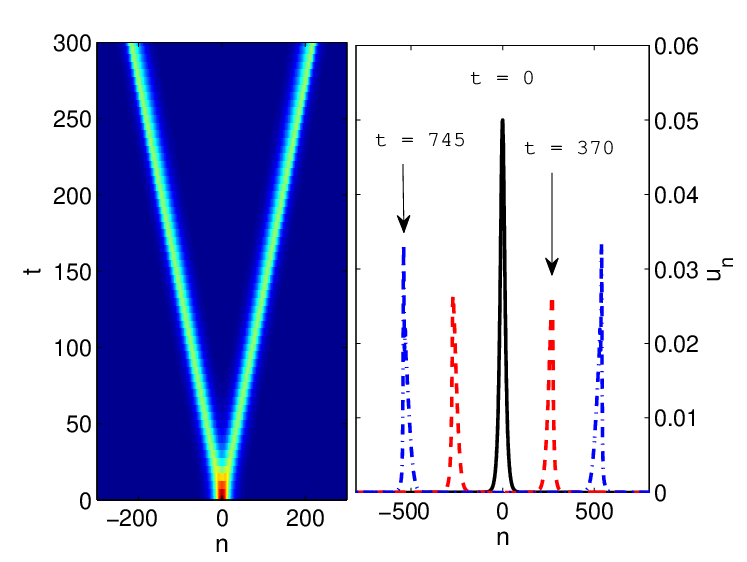
Refer to caption — Figure 1. Development of a shock-like structure with a smooth and localized initial condition of the granular crystal model (3) with $p=3/2$ and $\delta=0.1$ . A space-time contour plot is shown on the left and spatial profiles at time $t=0$ (solid black line), $t=370$ (red dashed line) and $t=750$ (blue dashed-dot line) are shown in the right panel. In both panels it can be seen that the pulse separates into two counter-propagating waves. A zoom of the wave before and after the point of shock development is shown in Fig. 2.

We now briefly discuss some analytical and numerical observations that stem from the leading order quasicontinuum approximation developed in Theorem 1.1. The continuum model

\partial^{2}_{T}A=\partial^{2}_{X}((\delta_{0}+A)^{p})

can be written as a system of conservation laws

\left.\begin{array}[]{cc}\partial_{T}A-\partial_{X}v&=0\\ \partial_{T}v-\partial_{X}[(\delta_{0}+A)^{p}]&=0\end{array}\right\}

(16)

These conservation laws have the form of a so-called p-system [10, 18]. Defining

U=\begin{pmatrix}A\\ v\end{pmatrix},\qquad F(U)=\begin{pmatrix}-v\\ -(\delta_{0}+A)^{p}\end{pmatrix}

we can express (16) as,

\partial_{T}U+\partial_{X}F(U)=0

or equivalently as

\partial_{T}U+DF(U)\partial_{X}U=0

(17)

where

DF(U)=\begin{pmatrix}0&-1\\ -p(\delta_{0}+A)^{p-1}&0\end{pmatrix}

which has the eigenvalues $\lambda_{\pm}(U)=\pm\sqrt{p(\delta_{0}+A)^{p-1}}$ . Thus, solutions of (4) will consist of two counter-propagating waves traveling with velocity $\pm\sqrt{p(\delta_{0}+A)^{p-1}}$ . Since the wave speed will depend on the amplitude of the solution, bell-shaped initial data will deform and steepen and a shock wave will form in finite time. Discrete shock-like structures (which we will simply call shock waves) have been studied in granular media, e.g. in homogeneous and periodic chains with $p=3/2$ and $\delta_{0}=0$ [5, 11]. In those works, however, the shock wave is generated by applying a velocity to a single bead [5] or by imparting velocity to the end of the chain continuously [11]. In this paper, the mechanism for the development of the shock wave is fundamentally different. It manifests from an arbitrary non-monotonically-increasing initial strain profile under precompression and given a sufficiently long time to develop.

A natural question is if the shock wave formation predicted by the continuum model (4) is also present in full system (3). Theorem 1.1 no longer applies in this case, as the the shock wave violates the required smoothness condition. Nonetheless, we carry out a numerical simulation to address the relevant question with a smooth initial condition. Figure 1 shows the development of a shock wave in the discrete model (3) with the initial condition $u_{n}(0)=a\,\mathrm{sech}(b\epsilon n),v_{n}(0)=0$ where $a,b\in\mathbb{R}$ are shape parameters. The wave propagation closely follows the theoretical expectation on the basis of the leading order quasicontinuum approximation. Moreover, the predicted velocity $\pm\sqrt{p(\delta_{0}+A)^{p-1}}$ proved to be very accurate (for example, there was less than a $\%0.01$ relative error in the case shown in Fig. 1).

We would like to make a direct comparison of the solutions of the continuum model and the discrete model. However, one has to be careful when using numerical approximations of the continuum model. For example, if one uses a finite difference approximation for a spatial discretization of (4), then we arrive at a model identical to the granular model (3). One could use other numerical schemes, such as those based on adding artificial dispersion [10], but we will proceed in an alternative way to predict the development of a shock wave. Using the velocity relationship $\pm\sqrt{p(\delta_{0}+A)^{p-1}}$ , we can construct the profile of the continuum model for an arbitrary time, starting with the left or right wave (once they are separated) as an initial profile, see Fig. 2. A numerical computation is used to separate the profiles (i.e. we simulate (4) with a finite difference method until separation but before the development of any shock wave, thus avoiding any issues with smoothness). The continuum model predicts a shock wave for any time past the point of non-single-valuedness, as shown in right panel Fig. 2.

In FPU lattices, it is well known that dispersive shocks can develop, in which microscopic oscillations spread out in space and time [6]. From Fig. 2 one clearly sees near the point of wave breaking the development of such oscillations, which are absent in the continuum model [6]. Thus, it would be relevant to extend works like [6] in order to better understand shock waves in the granular crystal model (3).

8. Justification of the KdV and NLS approximation

In this section we would like to contrast the previous result with approximation results for the KdV and NLS approximation. The major difference lies in the ratio between the amplitude and the precompression. For the KdV and NLS approximation this ratio is $\mathcal{O}(\varepsilon^{2})$ resp. $\mathcal{O}(\varepsilon)$ where $0<\varepsilon\ll 1$ is the small perturbation parameter, whereas for the quasicontinuum approximation the ratio is $\mathcal{O}(1)$ , i.e., of a comparable order. Since Eq. (10) is exactly of the form of the FPU systems considered in [2, 15] the approximation theorems of these papers also apply here. The subsequent solutions $u_{n}$ will be $\mathcal{O}(\varepsilon^{2})$ , resp. $\mathcal{O}(\varepsilon)$ and hence will always live in the ball of the convergence with radius $\delta_{0}$ if the perturbation parameter $0<\varepsilon\ll 1$ is chosen to be sufficiently small.

Even spatially periodic arrangements can be considered here, namely

\partial^{2}_{t}u_{n}=a_{n+1}(u^{p}_{n+1})-2a_{n}(u^{p}_{n})+a_{n-1}(u^{p}_{n-1})

(18)

with $a_{n}=a_{n+N}$ for a fixed $N$ .

We formulate the relevant approximation theorems in the homogeneous case $N=1$ . For the KdV approximation we have,

Theorem 8.1.

Let $A\in C(\left[0,T_{0}\right],H^{6})$ be a solution of the KdV equation $\partial_{T}A=\nu_{1}\partial^{3}_{X}A+\nu_{2}\partial_{X}(A^{2})$ with suitable chosen coefficients $\nu_{1},\nu_{2}\in\mathbb{R}$ . Then there exist $\varepsilon_{0}>0,\,C>0$ such that for all $\varepsilon\in(0,\varepsilon_{0})$ we have solutions $(u_{n})_{n\in\mathbb{Z}}$ of (18) with

\sup_{t\in[0,T_{0}/\varepsilon^{3}]}\sup_{n\in\mathbb{N}}\left|u_{n}(t)-\psi_{n}(t)\right|\leq C\varepsilon^{5/2},

where

\psi_{n}(t)=\varepsilon^{2}A\left(\varepsilon(n-\omega^{\prime}_{1}(0)t),\varepsilon^{3}t\right)

with $\omega_{1}(k)^{2}=\omega(k)^{2}b_{1}$ .

Proof.

The proof follows trivially from [2, Theorem 3.1] or [16]. We note there is no gap-opening in the small amplitude limit (i.e. the Heaviside function in the potential will play no role). ∎

The theorem can be generalized easily to an approximation theorem for two decoupled KdV equations describing counter-propagating waves, cf. [16].

For the NLS approximation we have,

Theorem 8.2.

Let $A\in C([0,T_{0}],H^{19})$ be a solution of the NLS equation $\partial_{T}A=i\nu_{1}\partial_{X}A+i\nu_{2}A\left|A\right|^{2}$ with suitable chosen coefficients $\nu_{1},\nu_{2}\in\mathbb{R}$ . Then there exist $\varepsilon_{0}>0,C>0$ such that for all $\varepsilon\in(0,\varepsilon_{0})$ we have solutions $(u_{n})_{n\in\mathbb{Z}}$ of (18) with

\sup_{t\in[0,T_{0}/\varepsilon^{2}]}\sup_{n\in\mathbb{N}}\left|u_{n}(t)-\psi_{n}(t)\right|\leq C\varepsilon^{3/2}

where

\psi_{n}(t)=\varepsilon A\left(\varepsilon(n-\omega^{\prime}_{1}(k_{0})t),\varepsilon^{2}t\right)e^{i(k_{0}n-\omega_{0}t)}+\textup{c.c.}

with $\omega_{1}(k)^{2}=\omega(k)^{2}b_{1}$

Proof.

The proof follows trivially from [2, Theorem 4.1] or [15, Theorem 1.1]. ∎

9. Conclusions and Future Challenges

The main result of this paper derives in a rigorous way (and with controllable corrections) the leading order quasicontinuum approximation for long wavelength solutions in the granular crystal model (3), in accordance with the formal derivation of Nesterenko [12]. As a technical assumption, we required the presence of a precompression factor (while the original Nesterenko model has been developed also in the case of the so-called “sonic vacuum” i.e., without precompression). One obvious avenue of future research is to investigate a proof without this assumption, which, however, would demand a fundamentally different technique than the one presented herein.

On the other hand, perhaps an even more important aspect of investigation concerns the well-posedness theory of the full Nesterenko model [12] or of the variant developed by Ahnert and Pikovsky in [1]. One important consequence of keeping only the leading order terms in the continuum model (as done herein) is the inability to capture the exact solitary wave solutions (which are known to exist in granular crystals [4, 3]) and are at the core of experimental observations in such systems [12, 17, 8]. The methods of this paper cannot be directly applied to that case, although we should note that we suspect that these higher order long wavelength models suffer (especially so in the case of precompression) from the type of pathologies that were identified by Rosenau and led him to devise appropriate regularizations [13, 14]; see also the more recent discussion of [9]. It would be especially relevant to consider such regularizations of the higher order long wavelength models both from a rigorous, as well as from a numerical perspective.

Another important consequence of keeping only first order terms in the continuum model is the prediction of the development of shock waves for a suitable (yet broad) class of initial data. Although the main theorem of this paper does not apply to the case of shock waves, due to smoothness considerations, numerical simulations indicate the steepening of relevant initial data towards a shock structure and suggest that this is indeed an issue worthy of further exploration, with an aim towards transferring these results to the discrete model. Indeed, it is known in FPU lattices that this procedure fails [6], due to the existence of high frequency oscillations (resulting from so-called dispersion shock waves). Thus, a different continuum model (than the one derived herein) will most likely be needed to fully characterize the emerging dispersive shock wave case. These topics are currently under consideration and will be reported in future publications.

Acknowledgments

The authors would like to thank Alexey Miroshnikov and Robin Young for helpful discussions regarding shock formation in the p-system. PGK acknowledges support from the US National Science Foundation under grant CMMI-1000337, the US Air Force under grant FA9550-12-1-0332, the Alexander von Humboldt Foundation, as well as the Alexander S. Onassis Public Benefit Foundation.

References

[1] K. Ahnert and A. Pikovsky, Compactons and chaos in strongly nonlinear lattices, Phys. Rev. E 79 (2009), 026209.
[2] Martina Chirilus-Bruckner, Christopher Chong, Oskar Prill, and Guido Schneider, Rigorous description of macroscopic wave packets in infinite periodic chains of coupled oscillators by modulation equations, Discrete Contin. Dyn. Syst. Ser. S 5 (2012), 879–901.
[3] R.L. English and J.M. Pego, On the solitary wave pulse in a chain of beads, Proceedings of the AMS 133 (2005), 1763–1768.
[4] G. Friesecke and J.A.D. Wattis, Existence theorem for solitary waves on lattices, Comm. Math. Phys. 161 (1994), 391–418.
[5] E. B. Herbold and V. F. Nesterenko, Shock wave structure in a strongly nonlinear lattice with viscous dissipation, Phys. Rev. E 75 (2007), 021304.
[6] Michael Herrmann and Jens D M Rademacher, Riemann solvers and undercompressive shocks of convex fpu chains, Nonlinearity 23 (2010), 277–304.
[7] Tosio Kato, The Cauchy problem for quasi-linear symmetric hyperbolic systems., Arch. Ration. Mech. Anal. 58 (1975), 181–205.
[8] P. G. Kevrekidis, Non-linear waves in lattices: past, present, future, IMA Journal of Applied Mathematics (2011), 389–423.
[9] P. G. Kevrekidis, I. G. Kevrekidis, A. R. Bishop, and E. S. Titi, Continuum approach to discreteness, Phys. Rev. E 65 (2002), 046613.
[10] Randall J. Leveque, Numerical Methods for Conservation Laws (Lectures in Mathematics), Birkhauser, 1992.
[11] A. Molinari and C. Daraio, Stationary shocks in periodic highly nonlinear granular chains, Phys. Rev. E 80 (2009), 056602.
[12] V.F. Nesterenko, Dynamics of heterogeneous materials, Springer-Verlag, New York, 2001.
[13] P. Rosenau, Dynamics of nonlinear mass-spring chains near the continuum limit, Physics Letters A 118 (1986), 222–227.
[14] P. Rosenau, Dynamics of dense lattices, Phys. Rev. B 36 (1987), 5868–5876.
[15] Guido Schneider, Bounds for the nonlinear Schrödinger approximation of the Fermi-Pasta-Ulam system, Appl. Anal. 89 (2010), no. 9, 1523–1539.
[16] Guido Schneider and C.Eugene Wayne, Counter-propagating waves on fluid surfaces and the continuum limit of the Fermi-Pasta-Ulam model., Fiedler, B. (ed.) et al., International conference on differential equations. Proceedings of the conference, Equadiff ’99, Berlin, Germany, August 1-7, 1999. Vol. 1. Singapore: World Scientific. 390-404, 2000.
[17] Surajit Sen, Jongbae Hong, Jonghun Bang, Edgar Avalos, and Robert Doney, Solitary waves in the granular chain, Physics Reports 462 (2008), no. 2, 21 – 66.
[18] J. Smoller, Shock waves and reaction-diffusion equations, Springer, New York, Heidelberg, Berlin, 1983.
[19] A. Stefanov and P. Kevrekidis, On the existence of solitary traveling waves for generalized hertzian chains, J. Nonlin. Sci. 22 (2012), 327–349.
[20] A. Stefanov and P. Kevrekidis, Traveling waves for monomer chains with precompression, Nonlinearity 26 (2013), 539–564.

Justification of Leading Order Quasicontinuum Approximations of Strongly Nonlinear Lattices

Abstract.

Key words and phrases:

1991 Mathematics Subject Classification

1. Introduction

Theorem 1.1.

2. Fourier transform as fundamental tool

Fourier transform on ℤ\mathbb{Z}:

Fourier transform on ℝ\mathbb{R}:

3. Derivation of the continuum model

4. Local existence and uniqueness of the continuum equation

Lemma 4.1.

Proof.

5. Estimates for the residual

Lemma 5.1.

Proof.

Lemma 5.2.

Proof.

6. The error estimates

7. Shock Formation in Granular Media

8. Justification of the KdV and NLS approximation

Theorem 8.1.

Proof.

Theorem 8.2.

Proof.

9. Conclusions and Future Challenges

Acknowledgments

References

Fourier transform on $\mathbb{Z}$ :

Fourier transform on $\mathbb{R}$ :