Markov Switching Component GARCH Model: Stability and Forecasting

N. Alemohammad S. Rezakhah S. H. Alizadeh Note: Faculty of Mathematics and Computer Science, Amirkabir University of Technology, Tehran, Iran. Email: n-alemohammad@aut.ac.ir, rezakhah@aut.ac.ir, sasan.h.alizadeh@qiau.ac.ir

Abstract

This paper introduces an extension of the Markov switching GARCH model where the volatility in each state is a convex combination of two different GARCH components with time varying weights. This model has the dynamic behaviour to capture the variants of shocks. The asymptotic behavior of the second moment is investigated and an appropriate upper bound for it is evaluated. The estimation of the parameters by using the Bayesian method via Gibbs sampling algorithm is studied. Finally we illustrate the efficiency of the model by simulation and empirical analysis. We show that this model provides a much better forecast of the volatility than the Markov switching GARCH model.

Keywords: GARCH models, Markov process, Stability, Component GARCH models, Forecasting, Bayesian inference, Griddy Gibbs sampling.

Mathematics Subject Classification: 60J10, 62M10, 62F15.

1 Introduction

In the past three decades, there has been a growing interest in using non linear time series models in finance and economy. For financial time series, the ARCH and GARCH models, introduced by Engle [11] and Bollerslev [7], are surely the most popular classes of volatility models. Although these models have been applied extensively in the modeling of financial time series, the dynamic structure of volatility can not be captured passably by such models. For more consistent volatility modeling, the models by time varying parameters are introduced. One class of such models is that of smooth transition GARCH models presented by Gonzalez-Rivera [14], Lubrano [23] (see also Hagerud [19] and Medeiros and Veiga [25]). These models can be considered as a valuable tool for including the asymmetry properties to negative and positive or small and big shocks in financial time series. The component GARCH models, introduced first by Ding and Granger [10], are also a generalization of the constant parameter GARCH model. In the structure of the component GARCH model ([10]), two different GARCH components contribute to the overall conditional variance at time t. One component has the high volatility (integrated variance component) and the other one has the low volatility. These models have been widely applied in modeling the financial time series (e.g. [24] and [12]). A generalization of the component GARCH model of Ding and Granger is the weighted GARCH model that is proposed by Bauwens and Storti [5]. In this model the weights of GARCH components are the functions of lagged values of the conditional standard deviation or squared past observations.

Another class is that of Markov switching models. These models are obtained by Merging (G)ARCH model with a Markov process, where each state of the Markov model allows a different (G)ARCH behavior. These models are introduced by Cai [8] and Hamilton and Susmel [18]. This feature extends the dynamic formulation of the model and potentially enables improving forecasts of the volatility [1]. Gray [15], Klaassen [21], Haas, Mittnik and Paolella [17] proposed different variants of Markov-Switching GARCH models. See also further studies, Abramson and Cohen [1], Alexander and Lazar [2] and Bauwens et al. [6].

In this paper we consider a Markov switching model that the volatility of each state is a convex combination of two GARCH regimes with time varying coefficients which is in effect of the previous observation. This model has the potential to switch between several regimes with various volatilities and also is able to model the time series with variants of shocks. The structure of the model makes a dynamic behavior in each regime to react differently to the species of shocks. For example in the high volatility regime, the model is able to have different responses to very high and high shocks and in low volatility regime different reactions to moderate and low shocks. We consider different weight functions for each state that allow volatility in each state to react differently to the shocks of equal size. As using all past observations for forecasting could increase the complexity of the model, we reduce the volume of calculations by proposing a dynamic programming algorithm. We derive necessary and sufficient conditions for stability and obtain an upper bound for the limit of the second moment by using the method of Abramson and Cohen [1] and Medeiros [25]. For the estimation of the parameters, we use the Bayesian inference via the Gibbs sampling. We compare the performance of our model with the Markov switching GARCH model. The Markov switching component GARCH model can forecast the conditional variance much better than MS-GARCH model.

The paper is organized as follows: in section 2 we introduce the Markov switching component GARCH model. Section 3 investigates the statistical properties of the model. Section 4 is devoted to the estimation of the parameters of the model. Section 5 is dedicated to the analyzing of the efficiency of the proposed model through simulation and the comparison of the forecast errors with the MS-GARCH model. The empirical applications and discussion are developed in section 6. Section 7 concludes.

2 Markov Switching Component GARCH Model

The Markov switching component GARCH model, MS-CGARCH, for time series $\{y_{t}\}$ is defined as

y_{t}=\varepsilon_{t}\sqrt{H_{t,Z_{t}}},\hskip 56.9055pt

(2.1)

where $\{\varepsilon_{t}\}$ are iid standard normal variables, $\{Z_{t}\}$ is an irreducible and aperiodic Markov chain on finite state space $E=\{1,2,\cdots,K\}$ with transition probability matrix $\;P=||p_{ij}||_{K\times K},\;$ where $\,p_{ij}=p(Z_{t}=j|Z_{t-1}=i),\;i,j\in\{1,\cdots,K\}$ , and stationary probability measure $\,\pi=(\pi_{1},\cdots,\pi_{K})^{\prime}.$ Also given that $Z_{t}=j$ , $H_{t,j}$ (the conditional variance in regime j) is driven by

H_{t,j}=w_{t,j}h_{1,t,j}+(1-w_{t,j})h_{2,t,j},

(2.2)

where

	$\displaystyle h_{1,t,j}=$	$\displaystyle a_{0j}+a_{1j}y^{2}_{t-1}+a_{2j}H_{t-1,j},$		(2.3)
	$\displaystyle h_{2,t,j}=$	$\displaystyle b_{0j}+b_{1j}y^{2}_{t-1}+b_{2j}H_{t-1,j},$		(2.4)

and each of the weights ( $w_{t,j}$ ) is a function of the past observation as

w_{t,j}=\frac{1-\exp(-\gamma_{j}|y_{t-1}|)}{1+\exp(-\gamma_{j}|y_{t-1}|)}\ \ \ \ \gamma_{j}>0,\ \ \ \

(2.5)

which is bounded , $0<w_{t,j}<1$ . The parameter $\gamma_{j}$ is called the slope parameter, that explains the speed of transition from one component to the other one: the higher $\gamma_{j}$ , the faster the transition. $H_{t-1,j}$ in (2.2) is the conditional variance of state m at time $t-1$ , that is a combination of conditional variances of both components at the state j. Since $\gamma_{j}>0$ , when the absolute value of $y_{t-1}$ increases, the impact of $h_{1,t,j}$ increases and consequently the effect of $h_{2,t,j}$ decreases and vice versa. Another good feature of our model is that it overcomes the problem of path dependency ¹¹ 1 Path dependency happens when the volatility of each regime at time t depends on the entire sequence of past regimes because of the recursive property of GARCH processes. (that is common in some kinds of MS-GARCH processes).
If $w_{t,j}$ becomes a constant value (for example when $\gamma_{j}$ tending to zero or infinity), the MS-CGARCH model will be a MS-GARCH model. In the case of single regime, if $a_{2.}=b_{2.}$ , our model is the generalization of the smooth transition GARCH model that is introduced by Lubrano [23].

It is assumed that $\{\varepsilon_{t}\}$ and $\{Z_{t}\}$ are independent. Sufficient conditions to guarantee strictly positive conditional variance are $a_{0j},b_{0j}$ to be positive and $a_{1j},a_{2j},b_{1j}\\ ,b_{2j}$ being nonnegative.

Let $\mathcal{I}_{t}$ be the observation set up to time t. The conditional density function of $y_{t}$ given past observations is obtained as follows:

$\displaystyle f(y_{t}\|\mathcal{I}_{t-1})=$	$\displaystyle\sum_{j=1}^{K}{f(y_{t},Z_{t}=j\|\mathcal{I}_{t-1})}$
	$\displaystyle=\sum_{j=1}^{K}{p(Z_{t}=j\|\mathcal{I}_{t-1})f(y_{t}\|\mathcal{I}_{t-1},Z_{t}=j)}$
	$\displaystyle=\sum_{j=1}^{K}{\alpha_{j}^{(t)}\phi(\frac{y_{t}}{\sqrt{H_{t,j}}})}$	(2.6)

in which $\alpha_{j}^{(t)}=p(Z_{t}=j|\mathcal{I}_{t-1})$ (that is obtained in next section), and $\phi(.)$ is the probability density function of the standard normal distribution.

3 Statistical Properties of the model

In this section, the statistical properties of the MS-CGARCH model are investigated and the conditional variance of the process is obtained. We show that the model, under some conditions on coefficients and transition probabilities , is asymptotically stable in the second moment. An appropriate upper bound for the limiting value of the second moment is obtained.

3.1 Forecasting

The forecasting volatility (conditional variance) of MS-CGARCH model is given by

Var(Y_{t}|\mathcal{I}_{t-1})=\sum_{j=1}^{K}{\alpha_{j}^{(t)}H_{t,j}}=\sum_{j=1}^{K}{\alpha_{j}^{(t)}(w_{t,j}h_{1,t,j}+(1-w_{t,j})h_{2,t,j})}.

(3.7)

This relation shows that the conditional variance of this model is affected by the changes in states, the volatility of components and the weight functions in each state.
At each time $t$ , $\alpha_{j}^{(t)}$ (in equation (2.6), (3.7)) can be obtained from a dynamic programming method based on forward recursion algorithm, proposed in remark (3.1).

Remark 3.1

The value of $\alpha_{j}^{(t)}$ is obtained recursively by

\alpha_{j}^{(t)}=\frac{\sum_{m=1}^{K}{f(y_{t-1}|Z_{t-1}=m,\mathcal{I}_{t-2})p(Z_{t-1}=m|\mathcal{I}_{t-2})}p_{m,j}}{\sum_{m=1}^{K}{f(y_{t-1}|Z_{t-1}=m,\mathcal{I}_{t-2})p(Z_{t-1}=m|\mathcal{I}_{t-2})}}.

(3.8)

Proof 3.1

As the hidden variables $\{Z_{t}\}_{t\geq 1}$ have Markov structure in the MS-CGARCH model, so

$\displaystyle\alpha_{j}^{(t)}=$	$\displaystyle p(Z_{t}=j\|\mathcal{I}_{t-1})=\sum_{m=1}^{K}{P(Z_{t}=j,Z_{t-1}=m\|\mathcal{I}_{t-1})}$
	$\displaystyle=\sum_{m=1}^{K}{p(Z_{t}=j\|Z_{t-1}=m,\mathcal{I}_{t-1})p(Z_{t-1}=m\|\mathcal{I}_{t-1})}$
	$\displaystyle=\sum_{m=1}^{K}{p(Z_{t}=j\|Z_{t-1}=m)p(Z_{t-1}=m\|\mathcal{I}_{t-1})}$
	$\displaystyle=\frac{\sum_{m=1}^{K}{f(\mathcal{I}_{t-1},Z_{t-1}=m)p_{m,j}}}{\sum_{m=1}^{K}{f(\mathcal{I}_{t-1},Z_{t-1}=m)}}$
	$\displaystyle=\frac{\sum_{m=1}^{K}{f(y_{t-1}\|Z_{t-1}=m,\mathcal{I}_{t-2})p(Z_{t-1}=m\|\mathcal{I}_{t-2})}p_{m,j}}{\sum_{m=1}^{K}{f(y_{t-1}\|Z_{t-1}=m,\mathcal{I}_{t-2})p(Z_{t-1}=m\|\mathcal{I}_{t-2})}},$	(3.9)

where

f(y_{t-1}|Z_{t-1}=m,\mathcal{I}_{t-2})=\phi(\frac{y_{t-1}}{\sqrt{H_{t-1,m}}}).\hskip 113.81102pt

3.2 Stability

In this subsection, we investigate the stability of the second moment of MS-CGARCH model. Indeed we are looking for an upper bound for the second moment of our model. The second moment of the model can be calculated as:

E(y^{2}_{t})=E(H_{t,Z_{t}})=E_{Z_{t}}[E_{t-1}(H_{t,Z_{t}}|z_{t})]\hskip 170.71652pt

=\sum_{z_{t}=1}^{K}{\pi_{z_{t}}E_{t-1}(H_{t,Z_{t}}|z_{t})}.\hskip 71.13188pt

(3.10)

$E_{t}(\cdot)$ denotes the expectation with respect to the information up to time t. Also for summarization, we shall use $E(\cdot|z_{t})$ and $p(\cdot|z_{t})$ to represent $E(\cdot|Z_{t}=z_{t})$ and $P(\cdot|Z_{t}=z_{t})$ , respectively, where $z_{t}$ is the realization of the state at time t. We investigate the conditional variance under the chain state, $m$ , as follows:

$\displaystyle E_{t-1}(H_{t,m}\|z_{t})$	$\displaystyle=E_{t-1}[w_{t,m}(a_{0m}+a_{1m}y^{2}_{t-1}+a_{2m}H_{t-1,m})\|z_{t}]\hskip 142.26378pt$
	$\displaystyle\hskip 56.9055pt+E_{t-1}[(1-w_{t,m})(b_{0m}+b_{1m}y^{2}_{t-1}+b_{2m}H_{t-1,m})\|z_{t}]$
	$\displaystyle=b_{0m}+\underbrace{b_{1m}E_{t-1}[y^{2}_{t-1}\|z_{t}]}_{I}+\underbrace{(a_{0m}-b_{0m})E_{t-1}[w_{t,m}\|z_{t}]}_{II}+\underbrace{b_{2m}E_{t-1}(H_{t-1,m}\|z_{t})}_{III}$
	$\displaystyle+\underbrace{(a_{1m}-b_{1m})E_{t-1}[w_{t,m}y^{2}_{t-1}\|z_{t}]}_{IV}+\underbrace{(a_{2m}-b_{2m})E_{t-1}(w_{t,m}H_{t-1,m}\|z_{t})}_{V}.$	(3.11)

The relation (II) in (3.11) can be interpreted as follows:

E_{t-1}[y^{2}_{t-1}|z_{t}]=\sum_{z_{t-1}=1}^{K}{\int_{S_{\mathcal{I}_{t-1}}}{y^{2}_{t-1}p(\mathcal{I}_{t-1}|z_{t},z_{t-1})p(z_{t-1}|z_{t})d\mathcal{I}_{t-1}}}

=\sum_{z_{t-1}=1}^{K}{p(z_{t-1}|z_{t})E_{t-1}[y^{2}_{t-1}|z_{t-1},z_{t}]},

(3.12)

where $S_{\mathcal{I}_{t-1}}$ is the support of $\mathcal{I}_{t-1}=(y_{1},\cdots,y_{t-1})$ . Since the expected value of $y^{2}_{t-1}$ is independent of any future state, so

E_{t-1}[y^{2}_{t-1}|z_{t-1},z_{t}]=E_{t-1}[y^{2}_{t-1}|z_{t-1}].

(3.13)

Also using the tower property of the conditional expectation, $E[E(Y|X,Z)|X]=E(Y|X)$ [see Grimmett and Stirzaker (2001, p. 69)], we have

E_{t-1}[y^{2}_{t-1}|z_{t-1}]=E_{t-2}[E_{t-1}(y^{2}_{t-1}|\mathcal{I}_{t-2},z_{t-1})|z_{t-1}]\hskip 264.6107pt

\hskip 73.97733pt=E_{t-2}[H_{t-1,Z_{t-1}}|z_{t-1}].\hskip 142.26378pt

(3.14)

The calculation of $E_{t-1}[w_{t,m}|z_{t}]$ , $E_{t-1}[w_{t,m}y^{2}_{t-1}|z_{t}]$ and $E_{t-1}(w_{t,m}H_{t-1,m}|z_{t})$ is a problem that can not be easily done, for this reason we will try to find an upper bound for them.

Upper bound to II. As $0<w_{t,m}<1$ , so an upper bound for the relation II in (3.11) is obtained by

(a_{0m}-b_{0m})E_{t-1}[w_{t,m}|z_{t}]\leq|a_{0m}-b_{0m}|<\infty.

(3.15)

The relation (III) can be specified as

b_{2m}E_{t-1}(H_{t-1,m}|z_{t})=b_{2m}{\int_{S_{\mathcal{I}_{t-1}}}{H_{t-1,m}p(\mathcal{I}_{t-1}|z_{t})d\mathcal{I}_{t-1}}}

=b_{2,m}\sum_{z_{t-1}=1}^{K}{p(z_{t-1}|z_{t})E_{t-2}(H_{t-1,m}|z_{t-1})}.

(3.16)

Upper bound to IV. Let $0<M<\infty$ be a constant, so

	$\displaystyle E_{t-1}[w_{t,z_{t}}y^{2}_{t-1}\|z_{t}]=$	$\displaystyle E_{t-1}[w_{t,z_{t}}y^{2}_{t-1}I_{\|y_{t-1}\|<M}\|z_{t}]$
		$\displaystyle+E_{t-1}[w_{t,z_{t}}y^{2}_{t-1}I_{\|y_{t-1}\|\geq M}\|z_{t}]$

in which

I_{x<a}=\left\{\begin{array}[]{ll}1&\textrm{if $x<a$}\\ 0&\textrm{otherwise.}\end{array}\right.

As by (2.5), $0<w_{t,z_{t}}<1$ and so

E_{t-1}[w_{t,z_{t}}y^{2}_{t-1}|z_{t}]\leq M^{2}+E_{t-1}[w_{t,z_{t}}y^{2}_{t-1}I_{|y_{t-1}|\geq M}|z_{t}],

also

	$\displaystyle E_{t-1}[w_{t,z_{t}}y^{2}_{t-1}I_{\|y_{t-1}\|\geq M}\|z_{t}]=$	$\displaystyle\int_{S_{\mathcal{I}_{t-2}},y_{t-1}\leq-M}{y^{2}_{t-1}[w_{t,z_{t}}]p(\mathcal{I}_{t-1}\|z_{t})d\mathcal{I}_{t-1}}$
		$\displaystyle+\int_{S_{\mathcal{I}_{t-2}},y_{t-1}\geq M}{y^{2}_{t-1}[w_{t,z_{t}}]p(\mathcal{I}_{t-1}\|z_{t})d\mathcal{I}_{t-1}},$

by (2.5),

\lim_{y_{t-1}\rightarrow+\infty}w_{t,z_{t}}=1,\ \ \ \ \ \ \ \ \lim_{y_{t-1}\rightarrow-\infty}w_{t,z_{t}}=1,

(3.17)

therefore according to the definition of limit at infinity, for a small number $\delta>0$ , there will exist a finite constant $M>0$ such that if $y_{t-1}\geq M$ , $|w_{t,z_{t}}-1|\leq\delta$ and if $y_{t-1}\leq-M$ , $|w_{t,z_{t}}-1|\leq\delta$ . Hence

	$\displaystyle E_{t-1}[w_{t,z_{t}}y^{2}_{t-1}I_{\|y_{t-1}\|\geq M}\|z_{t}]\leq\$	$\displaystyle(\delta+1)\int_{S_{\mathcal{I}_{t-2}},y_{t-1}\leq-M}{y^{2}_{t-1}p(\mathcal{I}_{t-1}\|z_{t})d\mathcal{I}_{t-1}}$
		$\displaystyle+(\delta+1)\int_{S_{\mathcal{I}_{t-2}},y_{t-1}\geq M}{y^{2}_{t-1}p(\mathcal{I}_{t-1}\|z_{t})d\mathcal{I}_{t-1}}.$

Since the distribution of the $\{\varepsilon_{t}\}$ is symmetric, then

	$\displaystyle(\delta+1)\int_{S_{\mathcal{I}_{t-2}},y_{t-1}\leq-M}{y^{2}_{t-1}p(\mathcal{I}_{t-1}\|z_{t})d\mathcal{I}_{t-1}}\leq$	$\displaystyle(\delta+1)\int_{S_{\mathcal{I}_{t-2}},-\infty<y_{t-1}<0}{y^{2}_{t-1}p(\mathcal{I}_{t-1}\|z_{t})d\mathcal{I}_{t-1}}$
		$\displaystyle=(\delta+1)\frac{E_{t-1}[y^{2}_{t-1}\|z_{t}]}{2}$

and

	$\displaystyle(\delta+1)\int_{S_{\mathcal{I}_{t-2}},y_{t-1}\geq M}{y^{2}_{t-1}p(\mathcal{I}_{t-1}\|z_{t})d\mathcal{I}_{t-1}}\leq$	$\displaystyle(\delta+1)\int_{S_{\mathcal{I}_{t-2}},0<y_{t-1}<\infty}{y^{2}_{t-1}p(\mathcal{I}_{t-1}\|z_{t})d\mathcal{I}_{t-1}}$
		$\displaystyle=(\delta+1)\frac{E_{t-1}[y^{2}_{t-1}\|z_{t}]}{2}.$

Therefor

(a_{1m}-b_{1m})E_{t-1}[w_{t,z_{t}}y^{2}_{t-1}|z_{t}]\leq|a_{1m}-b_{1m}|(M^{2}+(\delta+1)E_{t-1}[y^{2}_{t-1}|z_{t}]).

Upper bound to V. Since $0<w_{t,m}<1$ , so

(a_{2m}-b_{2m})E_{t-1}(w_{t,m}H_{t-1,m}|z_{t})\leq|a_{2m}-b_{2m}|E_{t-1}(H_{t-1,m}|z_{t}).

(3.18)

By replacing the obtained upper bounds and relations (3.12)-(3.14) in (3.11), the upper bound for $E_{t-1}(H_{t,Z_{t}}|z_{t})$ is acquired as:

$\displaystyle E_{t-1}(H_{t,m}\|z_{t})$	$\displaystyle\leq a_{0m}+\|a_{1m}-b_{1m}\|M^{2}$
	$\displaystyle+\sum_{z_{t-1}=1}^{K}{{[b_{1m}+\|a_{1m}-b_{1m}\|(\delta+1)]p(z_{t-1}\|z_{t})}E_{t-2}[H_{t-1,Z_{t-1}}\|z_{t-1}]}$
$\displaystyle+$	$\displaystyle\sum_{z_{t-1}=1}^{K}{{a_{2m}p(z_{t-1}\|z_{t})}E_{t-2}[H_{t-1,m}\|z_{t-1}]},$	(3.19)

in which by Bayes’ rule

p(z_{t-1}|z_{t})=\frac{\pi_{z_{t-1}}}{\pi_{z_{t}}}\{P_{z_{t-1}z_{t}}\},

where $P$ is the transition probability matrix. Let

{\bf{\Omega}}=[a_{01}+|a_{11}-b_{11}|M^{2},\cdots,\\ a_{0K}+|a_{1K}-b_{1K}|M^{2}]^{\prime},

(3.20)

be a vector with K component, ${\bf{C}}$ denotes a $K^{2}$ -by- $K^{2}$ block matrix as

{\bf{C}}=\left(\begin{array}[]{cccc}{\bf{C}_{11}}&{\bf{C}_{21}}&\cdots&{\bf{C}_{K1}}\\ {\bf{C}_{12}}&{\bf{C}_{22}}&\cdots&{\bf{C}_{K2}}\\ \vdots&&&\vdots\\ {\bf{C}_{1K}}&{\bf{C}_{2K}}&\cdots&{\bf{C}_{KK}}\\ \end{array}\right)

(3.21)

with each block given by

{\bf{C}_{jk}}=p(Z_{t-1}=j|Z_{t}=k)({\bf{u}}{\bf{e}}^{\prime}_{j}+{\bf{v}}),\ \ \ \ \ \ \quad\ j,k=1,\cdots,K,

(3.22)

where ${\bf{u}}=[b_{11}+(\delta+1)|a_{11}-b_{11}|,\cdots,b_{1K}+(\delta+1)|a_{1K}-b_{1K}|]^{\prime}$ , ${\bf{e}}_{j}$ is a K-by-1 vector of all zeros, except its jth element, which is one, and ${\bf{v}}$ is a diagonal K-by-K matrix with elements $[a_{21},\cdots,a_{2K}]$ on its diagonal.
Let $A_{t}(j,k)=E_{t-1}[H_{t,j}|Z_{t}=k]$ , $\textbf{A}_{t}=[A_{t}(1,1),A_{t}(2,1),\cdots,A_{t}(K,1),A_{t}(1,2),\cdots,\\ A_{t}(K,K)]$ be a $K^{2}$ -by-1 vector and consider $\dot{{\bf{\Omega}}}=({\bf{\Omega}}^{\prime},\cdots,{\bf{\Omega}}^{\prime})^{\prime}$ be a vector that is made of K vector ${\bf{\Omega}}$ .

Hence by (3.20)-(3.22) we have the following recursive inequality vector form for $\textbf{A}_{t}$ , as

\textbf{A}_{t}\leq\dot{{\bf{\Omega}}}+{\bf{C}}\textbf{A}_{t-1},\ \ \ t\geq 0.

(3.23)

with some initial conditions $\textbf{A}_{-1}.$
Let $\Pi=[\pi_{1}{\bf{e}}^{\prime}_{1},\cdots,\pi_{K}{\bf{e}}^{\prime}_{K}]$ and consider $\rho(A)$ denotes the spectral radius of a matrix A, then we have the following theorem for the stationarity condition of the MS-CGARCH model.

Theorem 3.1

Let $\{Y_{t}\}_{t=0}^{\infty}$ follows the MS-CGARCH model, defined by (2.1)-(2.5), the process is asymptotically stable in variance and $\lim_{t\rightarrow\infty}E(Y^{2}_{t})\leq{\bf{\Pi^{\prime}(I-{\bf{C}})^{-1}\dot{{\bf{\Omega}}}}}$ , if and only if $\rho({\bf{C}})<1.$

Proof 3.2

[1], By recursive inequality (3.23),

\textbf{A}_{t}\leq\dot{{\bf{\Omega}}}\sum_{i=0}^{t-1}{{\bf{C}}^{i}}+{\bf{C}}^{t}\textbf{A}_{0}:=\textbf{B}_{t}.\hskip 241.84842pt

(3.24)

By the matrix convergence theorem [22], a necessary and sufficient condition for the convergence of $\textbf{B}_{t}$ where $t\rightarrow\infty$ is $\rho({\bf{C}})<1$ ( the value of $\delta$ can be considered small enough to be negligible). Under this condition, ${\bf{C}}^{t}$ converges to zero as t goes to infinity and $\sum_{i=0}^{t-1}{{\bf{C}}^{i}}$ converges to $(I-{\bf{C}})^{-1}$ provided that matrix $(I-{\bf{C}})$ is invertible. So if $\rho({\bf{C}})<1$ ,

\lim_{t\rightarrow\infty}\textbf{A}_{t}\leq(I-{\bf{C}})^{-1}\dot{{\bf{\Omega}}}.\hskip 241.84842pt

By (3.10) the upper bound for the asymptotic behavior of unconditional variance is given by

lim_{t\rightarrow\infty}E(y^{2}_{t})\leq{\bf{\Pi^{\prime}(I-C)^{-1}}}\dot{{\bf{\Omega}}}.\hskip 227.62204pt

If $\rho({\bf{C}})\geq 1$ , $\textbf{B}_{t}$ goes to infinity with the growth of the time and it can not be possible to find an upper bound for the unconditional second moment of the model.

4 Estimation

In this section we describe the estimation of the parameters of the MS-CGARCH model. We consider Bayesian MCMC method using Gibbs algorithm by following methods of sampling of a hidden Markov process ([9] and [20]), MS-GARCH model and weighted GARCH model ([5] and [6] ) for estimation of the parameters.

Let $Y_{t}=(y_{1},\cdots,y_{t})$ and $Z_{t}=(z_{1},\cdots,z_{t})$ . For the case of two states, the transition probabilities are $\eta=(\eta_{11},\eta_{12},\eta_{21},\eta_{22})$ and the parameters of the model are $\theta=(\theta_{1},\theta_{2})$ , where $\theta_{k}=(a_{0k},b_{0k},a_{1k},b_{1k},a_{2k},b_{2k},\gamma_{k})$ for $k=1,2$ .

The purpose of Bayesian inference is to simulate from the distributions of the parameters and the state variables given the observations. As $Z=(z_{1},\cdots,z_{T})$ and $Y=(y_{1},\cdots,y_{T})$ , the posterior density of our model is:

p(\theta,\eta,Z|Y)\propto p(\theta,\eta)p(Z|\theta,\eta)f(Y|\theta,\eta,Z),

(4.25)

in which $p(\theta,\eta)$ is the prior of the parameters. The conditional probability mass function of $Z$ given the $(\theta,\eta)$ is independent of $\theta$ , so

$\displaystyle p(Z\|\theta,\eta)=$	$\displaystyle p(Z\|\eta_{11},\eta_{22})$
	$\displaystyle=\prod_{t=1}^{T}{p(z_{t+1}\|z_{t},\eta_{11},\eta_{22})}$
	$\displaystyle=p_{11}^{n_{11}}(1-p_{11})^{n_{12}}p_{22}^{n_{22}}(1-p_{22})^{n_{21}},$	(4.26)

where $n_{ij}=\#\{z_{t}=j|z_{t-1}=i\}$ . The conditional density function of $Y$ given the realization of $Z$ and the parameters is factorized in the following way:

f(Y|\eta,\theta,Z)=\prod_{t=1}^{T}{f(y_{t}|\theta,z_{t}=k,Y_{t-1})},\ \ \ k=1,2,

(4.27)

where the one step ahead of the predictive densities are:

f(y_{t}|\theta,z_{t}=k,Y_{t-1})=\frac{1}{\sqrt{2\pi H_{t,k}}}\exp(-\frac{y^{2}_{t}}{H_{t,k}}).

(4.28)

Since the posterior density (4.25) is not standard we can not sample it in a straightforward manner. Gibbs sampling of Gelfand and Smith [13] is a repetitive algorithm to sample consecutively from the posterior distribution. Under regularity conditions, the simulated distribution converges to the posterior distribution, (see e.g Robert and Casella [26]). The blocks of parameters are $\theta$ , $\eta$ and the realizations of $Z$ .
A brief description of the Gibbs algorithm: Let use the superscript $(r)$ on $Z,\,\theta$ and $\eta$ to denote the estimators of $Z$ , $\eta$ , and $\theta$ at the r-th iteration of the algorithm. Each iteration of the algorithm consists of three steps:
(i) Drawing an estimator random sample of the state variable $Z^{(r)}$ given $,\eta^{(r-1)},\ \theta^{(r-1)}$ .
(ii) Drawing a random sample of the transition probabilities $\eta^{(r)}$ given $Z^{(r)}$ .
(iii) Drawing a random sample of the $\theta^{(r)}$ given $Z^{(r)}$ and $\eta^{(r)}$ .

These steps are repeated until the convergency is obtained. In what follows sampling of each block is explained.

4.1 Sampling $z_{t}$

The purpose of this step is to obtain the sample of $p(z_{t}|\eta,\theta,Y_{t})$ that is performed by Chib[9], (see also [20]). Suppose $p(z_{1}|\eta,\theta,Y_{0},)$ be the stationary distribution of the chain,

p(z_{t}|\eta,\theta,Y_{t})\propto f(y_{t}|\theta,z_{t}=k,Y_{t-1})p(z_{t}|\eta,\theta,Y_{t-1}),

(4.29)

where the predictive density $f(y_{t}|\theta,z_{t}=k,Y_{t-1})$ is calculated by the relation (4.28) and by the law of total probability $p(z_{t}|\eta,\theta,Y_{t-1})$ is given by:

p(z_{t}|\eta,\theta,Y_{t-1})=\sum_{z_{t-1}=1}^{K}{p(z_{t-1}|\eta,\theta,Y_{t-1})\eta_{z_{t-1}z_{t}}}.

(4.30)

Given the filter probabilities ( $p(z_{t}|\eta,\theta,Y_{t})$ ), we run a backward algorithm, starting from $t=T$ that $z_{T}$ is derived from $p(z_{T}|\eta,\theta,Y)$ . For $t=T-1,\cdots,0$ the sample is derived from $p(z_{t}|z_{t+1},\cdots,z_{T},\theta,\eta,Y)$ ,which is obtained by

p(z_{t}|z_{t+1},\cdots,z_{T},\theta,\eta,Y)\propto p(z_{t}|\eta,\theta,Y_{t})\eta_{z_{t},z_{t+1}}.

To derive $z_{t}$ from $p(z_{t}|\cdot)=p_{z_{t}}$ is by sampling from the conditional probabilities (for example) $q_{1}=p(Z_{t}=1|Z_{t}\geq 1,.)$ which are given by

p(Z_{t}=1|Z_{t}\geq 1,.)=\frac{p_{1}}{\sum_{l=1}^{2}{p_{l}}}.

After generating a uniform (0,1) number $U$ , if $U\leq q_{1}$ then $z_{t}=1$ , otherwise $z_{t}=2$ .

4.2 Sampling $\eta$

This stage is devoted to sample $\eta=(\eta_{11},\eta_{22})$ from the posterior probability $p(\eta|\theta,Y_{t},Z_{t})$ that is independent of $Y_{t},\theta$ . We consider independent beta prior density for each of $\eta_{11}$ and $\eta_{22}$ . For example,

p(\eta_{11}|Z_{t})\propto p(\eta_{11})p(Z_{t}|\eta_{11})=\eta_{11}^{c_{11}+n_{11}-1}(1-\eta_{11})^{c_{12}+n_{12}-1},

where $c_{11}$ and $c_{12}$ are the parameters of Beta prior, $n_{ij}$ is the number of transition from $z_{t-1}=i$ to $z_{t}=j$ . In the same way the sample of $\eta_{22}$ is obtained.

4.3 Sampling $\theta$

The posterior density of $\theta$ given the prior $p(\theta)$ is given by:

p(\theta|Y,Z,\eta)\propto p(\theta)\prod_{t=1}^{T}{f(y_{t}|\theta,z_{t}=k,Y_{t-1})}=p(\theta)\prod_{t=1}^{T}{\frac{1}{\sqrt{2\pi H_{t,k}}}\exp(-\frac{y^{2}_{t}}{H_{t,k}})},

(4.31)

which is independent of $\eta$ . Since the conditional distribution of $\theta$ does not have a closed-form (because for example $p(a_{0k}|Y_{t},Z_{t},\theta_{-a_{0k}})$ , in which $\theta_{-a_{0k}}$ is the parameter vector without $a_{0k},$ contains $H_{t,k}$ , which is also a function of $a_{0k}$ . Therefor it can not be a normal density.) using the Gibbs sampling in this situation may be complicated. The Griddy Gibbs algorithm, that introduced by Ritter and Tanner (1992), can be a solution of this problem. This method is very applicable in researches (for example [4] , [5] and [6]).

Given samples at iteration $r$ the Griddy Gibbs at iteration $r+1$ proceeds as follows:

1. Select a grid of points, such as $a_{0i}^{1},a_{0i}^{2},\cdots,a_{0i}^{G}$ . Using (4.31), evaluate the conditional posterior density function $k(a_{0i|Z_{t},Y_{t},\theta_{-a_{0i}}})$ over the grid points to obtain the vector $G_{k}=(k_{1},\cdots,k_{G})$ .
2. By a deterministic integration rule using the G points, compute $G_{\Phi}=(0,\Phi_{2},\cdots,\Phi_{G})$ with

\Phi_{j}=\int_{a_{0i}^{1}}^{a_{0i}^{j}}{k(a_{01}|\theta_{-a_{0i}}^{(r)},Z^{(r)}_{t},Y_{t})da_{0i}},\ \ \ i=2,\cdots,G.

(4.32)

3. Simulate $u\sim U(0,\Phi_{G})$ and invert $\Phi(a_{0i}|\theta_{-a_{0i}}^{(r)},Z^{(r)}_{t},Y_{t})$ by numerical interpolation to obtain a sample $a_{0i}^{(r+1)}$ from $a_{0i}|\theta_{-a_{0i}}^{(r)},Z^{(r)}_{t},Y_{t}$ .
4. Repeat steps 1-3 for other parameters.

For the prior densities of all elements of $\theta$ , it can be can considered independent uniform densities over the finite intervals.

5 Simulation Results

In this section we provide some simulation results of MS-CGARCH model defined by equations (2.1)-(2.5) for two states. We simulate 300 sample from the following MS-CGARCH model:

y_{t}=\varepsilon_{t}\sqrt{H_{Z_{t},t}},\hskip 284.52756pt

(5.33)

where $\{\varepsilon_{t}\}$ is an iid sequence of standard normal variables, $\{Z_{t}\}$ is a Markov chain on finite state space $E=\{1,2\}$ with transition probability matrix

P=\left(\begin{array}[]{cc}.85&.15\\ .05&.95\\ \end{array}\right),

and

$\displaystyle H_{1,t}=$	$\displaystyle\frac{1-\exp(-2\|y_{t-1}\|)}{1+\exp(-2\|y_{t-1}\|)}(2.2+.75y^{2}_{t-1}+.15H_{1,t-1})+$
	$\displaystyle\hskip 113.81102pt[1-\frac{1-\exp(-2\|y_{t-1}\|)}{1+\exp(-2\|y_{t-1}\|)}](.7+.3y^{2}_{t-1}+.2H_{1,t-1}),$
$\displaystyle H_{2,t}=$	$\displaystyle\frac{1-\exp(-.5\|y_{t-1}\|)}{1+\exp(-.5\|y_{t-1}\|)}(.4+.15y^{2}_{t-1}+.1H_{2,t-1})+$
	$\displaystyle\hskip 113.81102pt[1-\frac{1-\exp(-.5\|y_{t-1}\|)}{1+\exp(-.5\|y_{t-1}\|)}](.2+.1y^{2}_{t-1}+.2H_{2,t-1}).$	(5.34)

The first state implies a higher conditional variance than the second one and in each state, the first component has the higher volatility than the other component.

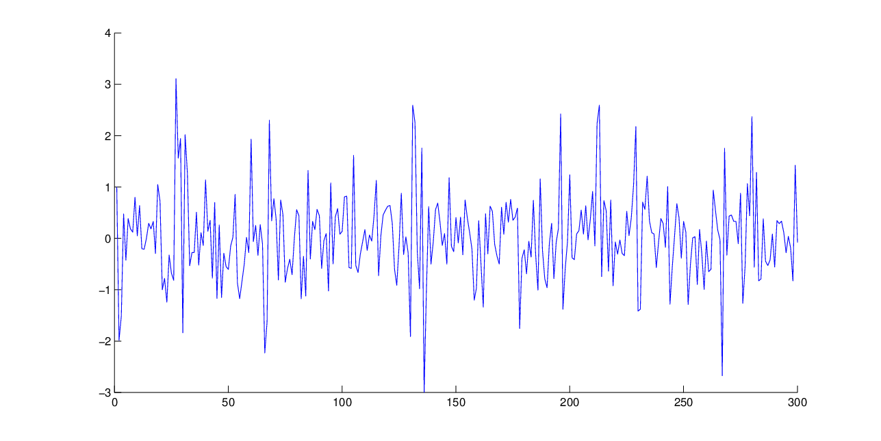
Refer to caption — Figure 1: Simulated time series of MS-CGARCH model.

In Table 1, we report summery statistics for simulated data and figure 1 shows the plot of the simulated time series.

Using the Bayesian inference, we estimate the parameters of the MS-CGARCH model. The prior density of each parameter is assumed to be uniform restricted over a finite interval (except for $\eta_{11}$ and $\eta_{22}$ , since they are drawn from the beta distribution). Table 2 demonstrates the performance of the estimation methods. The results of this table show that the standard deviation are small enough in most cases.

For clarifying the performance of MS-CGARCH model toward MS-GARCH model, We compare the forecasting volatility ( $E(Y^{2}_{t}|\mathcal{F}_{t-1})$ ) of each model with the squared observations. Figure 2 shows that the forecasting volatility of MS-CGARCH is much better than MS-GARCH model and the absolute forecast error (the difference between the forecasting volatility and the squared observations) of our model is often smaller than the MS-GARCH model. The root of mean squared error of the MS-GARCH and MS-CGARCH respectively are 0.738 and .483 and the mean absolute error of them are 0.510 and .3804.

Table 1: Descriptive statistics for the simulated data (sample size=300).

Mean	Std. dev.	Skewness	Maximum	Minimum	Kurtosis
0.034	0.860	0.289	3.109	-2.997	4.502

6 Empirical Applications

We apply the daily stock market index of Dow Jones industrial average (DJIA) from 07/10/2009 to 14/12/2010 (300 observations) and $S\&P500$ from 12/12/2006 to 22/02/2008 (300 observations) for estimation. Figures 3 demonstrates the stock market index and the percentage returns ²² 2 Percentage returns are defined as $r_{t}=100*\log(\frac{P_{t}}{P_{t-1}})$ , where $P_{t}$ is the index level at time t. of both DJIA and $S\&P500$ . It is evident that the stock market index of DJIA and $S\&P500$ have the divers of shocks. A summary of descriptive statistics of these returns are in Table 3.

Table 2: Results of the Bayesian Estimation of the simulated MS-CGARCH model.

	True values	Mean	Std. dev.
$a_{01}$	2.200	2.301	0.415
$a_{11}$	0.750	0.721	0.060
$a_{21}$	0.150	0.147	0.047
$b_{01}$	0.700	0.661	0.085
$b_{11}$	0.300	0.270	0.070
$b_{21}$	0.200	0.213	0.056
$a_{02}$	0.400	0.361	0.084
$a_{12}$	0.150	0.176	0.043
$a_{22}$	0.100	0.119	0.056
$b_{02}$	0.200	0.181	0.094
$b_{12}$	0.100	0.050	0.026
$b_{22}$	0.200	0.203	0.081
$\gamma_{1}$	2.000	2.01	0.603
$\gamma_{2}$	0.500	0.742	0.150
$\eta_{11}$	0.850	0.620	0.086
$\eta_{22}$	0.950	0.869	0.042

In Tables 4 and 5, the posterior means and standard deviations from the estimation of MS-CGARCH and MS-GARCH models for DJIA and $S\&P500$ daily returns are reported. The results of estimating MS-GARCH in both cases (DJIA and $S\&P500$ daily returns) show that the first regime is the high volatility regime. In the high volatility state, the conditional variance is more sensitive to recent shocks ( $a_{11}>a_{21}$ ) and less persistence ( $a_{21}<a_{22}$ ) than the low volatility regime. Also the outcomes of estimating MS-CGARCH (Tables 4 and 5) show that the first regime is the high volatility state that in each state the first component is higher volatile than the second one. The values of $\gamma_{1}$ and $\gamma_{2}$ show the speed of transition (in each regime) from one component to the other one. This specification causes the MS-CGARCH to be more flexible than the MS-GARCH to capture the variants of shocks: very high, high, moderate and low shocks. Indeed the MS-CGARCH model is able to model the gradual changes in high and low volatile states by the effect of their components in each state.
We compare the forecasting volatility of each model with the squared returns. Figure 4 and 5 show that the forecasting volatility of MS-CGARCH is much better than MS-GARCH model. Table 6 reports the measures of performance forecasting, the mean absolute error and root of mean squared error, for both MS-CGARCH and MS-GARCH models. Based on the results given in Table 6, the MS-CGARCH model has a much better forecast than MS-GARCH model.

Table 3: Descriptive statistics of DJIA and

S\&P500

stock market returns.

	Mean	Std. dev.	Skewness	Maximum	Minimum	Kurtosis
DJIA	0.05	1.01	-0.18	3.82	-3.67	4.76
$S\&P500$	-0.01	1.04	-0.54	2.87	-3.53	4.14

Table 4: Posterior means and standard deviations (DJIA daily returns).

	MS-CGARCH		MS-GARCH
	Mean	Std.dev.	Mean	Std.dev
$a_{01}$	3.150	0.590	1.859	0.316
$a_{11}$	0.651	0.145	0.504	0.102
$a_{21}$	0.094	0.043	0.216	0.054
$b_{01}$	0.821	0.142	$\_$	$\_$
$b_{11}$	0.306	0.061	$\_$	$\_$
$b_{21}$	0.277	0.050	$\_$	$\_$
$a_{02}$	0.658	0.157	0.498	0.091
$a_{12}$	0.296	0.054	0.189	0.055
$a_{22}$	0.203	0.053	0.242	0.071
$b_{02}$	0.291	0.049	$\_$	$\_$
$b_{12}$	0.092	0.049	$\_$	$\_$
$b_{22}$	0.334	0.087	$\_$	$\_$
$\gamma_{1}$	1.554	0.307	$\_$	$\_$
$\gamma_{2}$	0.756	0.136	$\_$	$\_$
$\eta_{11}$	0.806	0.140	0.542	0.092
$\eta_{22}$	0.941	0.038	0.899	0.031

Table 5: Posterior means and standard deviations (

S\&P500

daily returns).

	MS-CGARCH		MS-GARCH
	Mean	Std.dev.	Mean	Std.dev
$a_{01}$	2.016	0.548	1.330	0.329
$a_{11}$	0.609	0.132	0.454	0.102
$a_{21}$	0.184	0.050	0.303	0.062
$b_{01}$	0.767	0.129	$\_$	$\_$
$b_{11}$	0.286	0.053	$\_$	$\_$
$b_{21}$	0.352	0.059	$\_$	$\_$
$a_{02}$	0.622	0.145	0.500	0.092
$a_{12}$	0.249	0.092	0.162	0.069
$a_{22}$	0.130	0.056	0.232	0.065
$b_{02}$	0.313	0.058	$\_$	$\_$
$b_{12}$	0.086	0.049	$\_$	$\_$
$b_{22}$	0.315	0.077	$\_$	$\_$
$\gamma_{1}$	1.856	0.505	$\_$	$\_$
$\gamma_{2}$	0.725	0.126	$\_$	$\_$
$\eta_{11}$	0.774	0.086	0.821	0.065
$\eta_{22}$	0.915	0.027	0.936	0.022

Table 6: Measures of performance forecasting.

	DJIA		$S\&P500$
	MS-GARCH	MS-CGARCH	MS-GARCH	MS-CGARCH
RMSE	1.281	0.834	1.169	0.902
MAE	0.940	0.687	0.904	0.723

7 Conclusion

In this paper a generalization of the MS-GARCH model has been presented where the conditional variance in each state is a convex combination of two different GARCH components with time varying coefficients, one of the component with higher volatility than the other component. The structure of the model makes a dynamic behavior in each regime to react differently to the species of shocks. Our model can provide more better forecast of volatility toward MS-GARCH model. For the estimation of parameters we have applied the Bayesian estimation algorithm. We provide a simple necessary and sufficient condition for the existence of an upper bound for the second moment.

This work has the potential to be applied in the context of financial time series. The empirical distribution of daily returns doesn’t generally have a Gaussian distribution. They have fat tails densities (they are called leptokurtic). One of the extending of this work is considering the fat tail densities instead of Gaussian distribution, that can cause better modeling of the financial time series. Also we can generalize this model by allowing an ARMA structure for the conditional mean.

References

[1] Abramson, A. Cohen, I. (2007). On the stationarity of Markov-Switching GARCH processes, Econometric Theory, 23, 485-500.
[2] Alexander, C. Lazar, E. (2008). Markov-Switching GARCH diffusion, ICMA Center Discussion Paper in Finance 2008-01, University of Reading.
[3] Alizadeh, S. H. Rezakhah, S. (2013). Hidden Markov mixture autoregressive models:stability and moments,Communications in Statistics- Theory and Methods, 42:6, 1087-1104.
[4] Bauwens, L. Lubrano, M. (1998). Bayesian inference on GARCH models using the Gibbs sampler, Econometrics journal, 1, 23-46.
[5] Bauwens, L. Storti, G. (2009). A component GARCH model with time varying weights, Studies in Nonlinear Dynamics and Econometrics, 13 (2), Article 3.
[6] Bauwens, L. Preminger, A. Rombouts, V.K. (2010). Theory and inferencefor Markov switching GARCH model , Econometrics journal, 13, 218-244.
[7] Bollerslev, T. (1986). Generalized autoregressive conditional heteroscedasticity, Journal of Econometrics, 31, 307-327.
[8] Cai, J. (1994). A markonv model of switching -regime ARCH, Journal of Business and Economic Statistics, 12, 309-316.
[9] Chib, S. (1996). Calculating posterior distributions and model estimates in Markov mixture models, Journal of Econometrics, 75, 79-97.
[10] Ding, Z. Granger, C.W.J. (1996).Modeling volatility persistence of speculative returns: a new approach, Journal of Econometrics, 173, 185-215.
[11] Engle, R. F. (1982). Autoregressive conditional heteroscedasticity with estimates of the variance of united kingdom inflation, Econometrica, 50, 987-1007. 3, 103-106.
[12] Engle, R. F. Rangel, J. (2008). The Spline-GARCH model for low frequency volatility and its global macroeconomic causes , Review of Financial Studies, 21, 1187-1222.
[13] Gelfand, A. Smith, A. (1990). Sampling based approaches to calculating marginal densities, Journal of American Statistical Assosiation, 85, 398-409.
[14] Gonzalez-Rivera, G. (1998). Smooth transition GARCH models, Studies in Nonlinear Dynamics and Econometrics, 3, 61-78.
[15] Gray, S. F. (1996). Modeling the conditional distribution of interest rates as a regime-switching process, Journal of Financial Economics, 42, 27-62.
[16] Grimmett, G. Stirzaker, D. (2001). Probability and random processes, Oxford University press, New York.
[17] Haas, M. Mittnik, S. Paolella, M.S. (2004). A new approach to markov-switching GARCH models, Journal of Financial Econometrics, 2, 493-530.
[18] Hamilton, J. D. Susmel, R. (1994). Autoregressive conditional heteroskedasticity and changes in regime, Journal of Econometrics, 64, 307-333.
[19] Hagerud, G. (1997). A smooth transition ARCH model for asset returns, SSE/EFI, Working Paper Series in Economic and Finance, No.162.
[20] Kaufman, S. Fruhwirth-Schnatter, S. (2002). Bayesian analysis of switching ARCH models , Journal of Time Series Analysis, 23, 425-458.
[21] Klaassen, F. (2002). Improving GARCH volatility forecasts with regime-switching GARCH, Empirical Economics 27, 363-394.
[22] Lancaster, P. Tismenetsky, M. (1985). The theory of matrices, 2nd ed, Academic press.
[23] lubrano, M. (2001). Smooth transition GARCH models: a Bayesian approach mixture models, Recherches Economiques de Louvain, 67, 257-287.
[24] Maheu, J. (2005). Can GARCH models capture long range dependence?, Studies in Nonlinear Dynamics and Econometrics, 9 (4), Article 1.
[25] Medeiros, M.C. Veiga, A. (2009). Modeling multiple regimes in financial volatility with a flexible coefficient GARCH(1,1), Journal of Econometric Theory, 25, 117-161.
[26] Robert, C. Casella, G. (2004). Monte carlo statistical methods, New York: Springer.

$\displaystyle f(y_{t}\|\mathcal{I}_{t-1})=$	$\displaystyle\sum_{j=1}^{K}{f(y_{t},Z_{t}=j\|\mathcal{I}_{t-1})}$
	$\displaystyle=\sum_{j=1}^{K}{p(Z_{t}=j\|\mathcal{I}_{t-1})f(y_{t}\|\mathcal{I}_{t-1},Z_{t}=j)}$
	$\displaystyle=\sum_{j=1}^{K}{\alpha_{j}^{(t)}\phi(\frac{y_{t}}{\sqrt{H_{t,j}}})}$	(2.6)

$\displaystyle\alpha_{j}^{(t)}=$	$\displaystyle p(Z_{t}=j\|\mathcal{I}_{t-1})=\sum_{m=1}^{K}{P(Z_{t}=j,Z_{t-1}=m\|\mathcal{I}_{t-1})}$
	$\displaystyle=\sum_{m=1}^{K}{p(Z_{t}=j\|Z_{t-1}=m,\mathcal{I}_{t-1})p(Z_{t-1}=m\|\mathcal{I}_{t-1})}$
	$\displaystyle=\sum_{m=1}^{K}{p(Z_{t}=j\|Z_{t-1}=m)p(Z_{t-1}=m\|\mathcal{I}_{t-1})}$
	$\displaystyle=\frac{\sum_{m=1}^{K}{f(\mathcal{I}_{t-1},Z_{t-1}=m)p_{m,j}}}{\sum_{m=1}^{K}{f(\mathcal{I}_{t-1},Z_{t-1}=m)}}$
	$\displaystyle=\frac{\sum_{m=1}^{K}{f(y_{t-1}\|Z_{t-1}=m,\mathcal{I}_{t-2})p(Z_{t-1}=m\|\mathcal{I}_{t-2})}p_{m,j}}{\sum_{m=1}^{K}{f(y_{t-1}\|Z_{t-1}=m,\mathcal{I}_{t-2})p(Z_{t-1}=m\|\mathcal{I}_{t-2})}},$	(3.9)

$\displaystyle E_{t-1}(H_{t,m}\|z_{t})$	$\displaystyle=E_{t-1}[w_{t,m}(a_{0m}+a_{1m}y^{2}_{t-1}+a_{2m}H_{t-1,m})\|z_{t}]\hskip 142.26378pt$
	$\displaystyle\hskip 56.9055pt+E_{t-1}[(1-w_{t,m})(b_{0m}+b_{1m}y^{2}_{t-1}+b_{2m}H_{t-1,m})\|z_{t}]$
	$\displaystyle=b_{0m}+\underbrace{b_{1m}E_{t-1}[y^{2}_{t-1}\|z_{t}]}_{I}+\underbrace{(a_{0m}-b_{0m})E_{t-1}[w_{t,m}\|z_{t}]}_{II}+\underbrace{b_{2m}E_{t-1}(H_{t-1,m}\|z_{t})}_{III}$
	$\displaystyle+\underbrace{(a_{1m}-b_{1m})E_{t-1}[w_{t,m}y^{2}_{t-1}\|z_{t}]}_{IV}+\underbrace{(a_{2m}-b_{2m})E_{t-1}(w_{t,m}H_{t-1,m}\|z_{t})}_{V}.$	(3.11)

$\displaystyle E_{t-1}(H_{t,m}\|z_{t})$	$\displaystyle\leq a_{0m}+\|a_{1m}-b_{1m}\|M^{2}$
	$\displaystyle+\sum_{z_{t-1}=1}^{K}{{[b_{1m}+\|a_{1m}-b_{1m}\|(\delta+1)]p(z_{t-1}\|z_{t})}E_{t-2}[H_{t-1,Z_{t-1}}\|z_{t-1}]}$
$\displaystyle+$	$\displaystyle\sum_{z_{t-1}=1}^{K}{{a_{2m}p(z_{t-1}\|z_{t})}E_{t-2}[H_{t-1,m}\|z_{t-1}]},$	(3.19)

$\displaystyle p(Z\|\theta,\eta)=$	$\displaystyle p(Z\|\eta_{11},\eta_{22})$
	$\displaystyle=\prod_{t=1}^{T}{p(z_{t+1}\|z_{t},\eta_{11},\eta_{22})}$
	$\displaystyle=p_{11}^{n_{11}}(1-p_{11})^{n_{12}}p_{22}^{n_{22}}(1-p_{22})^{n_{21}},$	(4.26)