Computing Severi Degrees with Long-edge Graphs

The motivating question for this article is classical and well-known, namely to determine the number $N^{d,\delta}$ of (possibly reducible) curves in $\mathbb{P}^{2}_{\mathbb{C}}$ of degree $d$ having $\delta$ nodes and passing through $\dfrac{d(d+3)}{2}-\delta$ general points. This number $N^{d,\delta}$ is the degree of the Severi variety. When $d\geq\delta+2$, the curves in question are irreducible, so that $N^{d,\delta}$ coincides with the Gromov–Witten invariant $N_{d,g}$, where $g=\dfrac{(d-1)(d-2)}{2}-\delta$.

Despite its long history, there continues to be interest in the Severi degree and much recent activity surrounding it. In [3] Di Francesco and Itzykson conjectured that $N^{d,\delta}$ is given by a node polynomial $N_{\delta}(d)$ for sufficiently large $d$ and fixed $\delta$. The polynomiality of $N^{d,\delta}$ became part of Göttsche’s larger conjecture [5, Conjecture 4.1]—recently established by Tzeng in [14] and independently by Kool, Shende, Thomas [8]—regarding the existence of universal polynomials enumerating curves on smooth projective surfaces. The so-called threshold of polynomiality, i.e., the value $d^{*}$ such that the Severi degree $N^{d,\delta}$ is given by a polynomial for all $d\geq d^{*}$, has been steadily lowered. In the proof of Theorem 5.1 of [4], Fomin and Mikhalkin showed that $d^{*}\leq 2\delta$; this was improved to $d^{*}\leq\delta$ by the first author in [1]. In the past year the bound for $d^{*}$ was sharpened still further to at most $\lceil\delta/2\rceil+1$ (for $\delta\geq 3$) by Kleiman and Shende in [7]; this result establishes the threshold value conjectured by Göttsche in [5].

In addition to knowing the value of $d$ that ensures that $N^{d,\delta}$ is given by a polynomial is, of course, the issue of determining the node polynomials exactly. The node polynomials for the small numbers of nodes were known in the 19th century:

The node polynomials for $\delta=4,5,6$ were obtained by Vainsencher in [15], for $\delta=7,8$ by Kleiman and Piene in [6], and by the first author for $\delta\leq 14$ in [1].

We are particularly interested in the generating series for Severi degrees

and its formal logarithm

Writing the coefficients of $\mathcal{Q}(d)$ explicitly,

where the sum is over ordered partitions $\delta=\delta_{1}+\cdots+\delta_{p}$. For $d$ sufficiently large and $\delta$ fixed, $N^{d,\delta}$ is given by a polynomial of degree $2\delta$. Thus, a priori one would expect $Q^{d,\delta}$ likewise to be a polynomial of degree $2\delta$. However, $Q^{d,\delta}$ quite unexpectedly turns out to be quadratic. This is a consequence of the Göttsche–Yau–Zaslow Formula [5, Conjecture 2.4] (see also [11] and [12]), rather recently proved by Tzeng [14, Theorem 1.2] using very sophisticated techniques. One goal of this paper is to establish the quadraticity of $Q^{d,\delta}$, for $d$ sufficiently large and fixed $\delta$, in an elementary combinatorial way.

In Section 2 we describe what we call a long-edge graph, the main combinatorial tool to determine Severi degrees. A long-edge graph is in fact nothing other than an ordered collection of templates, as defined in [4] and [1]. They were used there to calculate Gromov–Witten invariants, Severi degrees, and node polynomials, but the perspective we take here is slightly different. In Section 3, we establish Theorem 3.7, which shows that a certain polynomial constructed from a long-edge graph is linear. Then in Section 4 we discuss templates from scratch and see that the quadraticity of $Q^{d,\delta}$ follows, since it is a discrete integral of the linear polynomial of Theorem 3.7. Finally, in Section 5, we explain how long-edge graphs arise from the tropical-geometric computation of Severi degrees, via the notion of floor diagrams.

One would hope to exploit the relationship between the quantities $N^{d,\delta}$ and $Q^{d,\delta}$ by inverting (1.2):

Explicitly, this gives

again summing over ordered partitions $\delta=\delta_{1}+\cdots+\delta_{p}$. Knowing that the quantities $Q^{d,\delta}$ are quadratic in $\delta$ (and in fact obtained from certain linear quantities, as explained below), and that only templates need to be used, one should be able to efficiently calculate the Severi degrees. What is needed is a way to calculate these quadratic quantities in some simple way from the graph-theoretic combinatorics laid out herein, rather than from the cumbersome definition (1.3). We intend to consider this problem further.

While our formulas for $Q^{d,\delta}$ are evidently not positive, a natural question is to find an inherently positive formula for the $Q^{d,\delta}$. This would be very desirable, as it might give further insight in “natural building blocks” of long-edge graphs and floor diagrams, in regard of identity (1.4). We also note that, in [9], F. Liu has recently and independently provided a combinatorial proof of the quadraticity of $Q^{d,\delta}$.

We express appreciation to our colleagues Sergei Chmuntov, Kyungyong Lee, Boris Pittel, and Kevin Woods for their helpful comments and suggestions regarding this work. Via the website MathOverflow, we received valuable insights into certain combinatorial issues, especially in postings by Will Sawin, Richard Stanley, Gjergji Zaimi, and David Speyer. We thank Eduardo Esteves, Dan Edidin, Abramo Hefez, Ragni Piene, and Bernd Ulrich for arranging a most stimulating 12th ALGA Meeting and to IMPA for hosting it. We are grateful to the referee for very useful comments that improved our exposition. Finally, we offer our sincere gratitude to Steven Kleiman and Aron Simis for their many years of mathematical stimulation and guidance.

Consider an edge-weighted multigraph $G$ on a vertex set indexed by the set of nonnegative integers $\{0,1,2,\dots\}$. If $e$ is an edge between vertex $i$ and vertex $j$, we define the length $l(e)$ of $e$ to be $l(e)=|i-j|$. Denote the weight of $e$ by $w(e)$.

For each nonnegative integer $i$, let

the sum taken over all edges lying over the interval $[i,i+1]$, i.e., edges beginning at or to the left of $i$, and ending at or to the right of $i+1$.

Note that if a long-edge graph $G$ satisfies criterion (3) in Definition 2.2, then there is some value of $d$ for which it is allowable, and that if $G$ is allowable for a particular value of $d$, it is allowable for all $d^{\prime}>d$ as well.

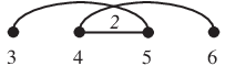
If $G$ is allowable for $d$, then we obtain its extended graph $\ext_{d}(G)$ by adding short edges to $G$ as follows: for each $i\leq d$, add $i-w_{i}$ such edges over the interval $[i,i+1]$. Note that in $\ext_{d}(G)$ the number of edges over $[i,i+1]$ will be exactly $i$ (counting each edge with its multiplicity). If we subdivide each edge of $\ext_{d}(G)$ by introducing one new vertex, we obtain a graph which we denote by $G^{\prime}_{d}$. An ordering of $G^{\prime}_{d}$ is a linear ordering of its vertices that extends the ordering of the vertices $\{0,1,2,\dots\}$ of $G$. (See Figure 2.) Two such orderings are considered equivalent if there is an automorphism of $G^{\prime}_{d}$ preserving the vertices of $G$.

If $G$ is allowable for $d$, then we define

remarking that this is independent of $d$ (as long as the graph is allowable for $d$). If $G$ is not allowable for $d$, then let $N^{d,G}=0$.

The significance of the constructions above is that they enable a combinatorial calculation of the Severi degrees of $\mathbb{P}^{2}$.

Although $N^{d,G}$ is the quantity which enters into Theorem 2.5, for purposes of calculation we often find it more convenient to work with an “automorphism-free” and “multiplicity-free” quantity. Suppose that the edges of $G$ have been labeled. Then (in the allowable cases) we define $N_{*}^{d,G}$ to be the number of orderings of $G^{\prime}_{d}$, so that

where $\alpha(G)$ is the number of automorphisms of $G$ when the edges are unlabeled. (The vertices remain labeled, however.) See Figure 3 for an example. Note that the short edges added to create $G^{\prime}_{d}$ are considered to be unlabeled. Any of these short edges which lie completely to the left or right of the edges of $G$ are irrelevant in the calculation of $N^{d,G}$; going forward, therefore, we usually will not display such edges.

To calculate $N^{d,G}$ for more complicated graphs, it is useful to work with distributions of the new vertices on the long edges. A distribution is a function $\Delta$ that associates, to each edge $e$ of $G$, one of the $l(e)$ intervals over which it lies. We say that an ordering of $G^{\prime}_{d}$ is consistent with $\Delta$ if, in this ordering, each new long-edge vertex introduced by the subdivision process (as described above) lies within the interval specified by $\Delta$. Let

noting as before that this number is independent of $d$, as long as the graph is allowable for $d$. Again we declare $N^{d,(G,\Delta)}=0$ when $G$ is not allowable for $d$. Summing over all possible distributions, we have

As above we often find it more convenient to work with the automorphism- and multiplicity-free quantity $N_{*}^{d,(G,\Delta)}$, noting that

where $\alpha(G,\Delta)$ is the number of automorphisms of $G$ consistent with $\Delta$. Since the short edges added to create $G^{\prime}_{d}$ are considered to be unlabeled and therefore indistinguishable (when they lie over the same interval), we have

where $m_{i}$ is the number of times that $[i,i+1]$ appears as a value of $\Delta$, and where $(i-w_{i}+m_{i})_{m_{i}}$ indicates a falling factorial (i.e., $(a)_{m}=a(a-1)\cdots(a-m+1)$ and we take $(a)_{0}$ to be $1$). The product in formula (2.7) is taken over all $i\geq 1$; however, all but finitely many factors have value $1$.

If we translate a long-edge graph $G$ rightward by $k$ units, we obtain another long-edge graph $G[k]$, which we will call an offset of $G$. In Example 2.6, the graphs $\text{Cyc}[k]$ and $\text{Stub}[k]$ are offsets of the graphs shown in Figure 6, which we call the cyclops template and the stub template. (The general notion of a template is explained in Section 4. The nomenclature originates with [4].) If $\Delta$ is a distribution of $G$, then $\Delta[k]$ is the distribution of $G[k]$ defined in the obvious way: if $\Delta(e)=[i,i+1]$ then $\Delta(e[k])=[k+i,k+i+1]$. Note that, for any $G$, we may choose a sufficiently large offset $k$ so that $G[k]$ satisfies criterion (3) of Definition 2.2.

Let $G$ be a long-edge graph satisfying criterion (3) of Definition 2.2; let $n$ be the number of edges of $G$ and let $\Edge(G)$ denote the set of edges. For each subset $E$ of $\Edge(G)$, consider the subgraph with these edges; for simplicity we also denote it by $E$. Note that any distribution $\Delta$ is inherited by $E$. We now consider, for each $d$, the alternating sums

and

summing in both instances over all unordered partitions $\mathcal{P}$ of $\Edge(G)$, taking products over the blocks $E$ of $\mathcal{P}$, and denoting by $p$ the number of blocks. In view of Proposition 2.8, we know that $Q^{d,(G,\Delta)}$ is a polynomial whose degree is at most $n$. In this section we show that, surprisingly, it is linear.

The automorphisms make the formulas in (3.1) and (3.2) look somewhat awkward, but if we use instead the automorphism- and multiplicity-free quantity

then (3.2) becomes

To provide some motivation for considering the particular alternating sums in (3.1) and (3.2), we show how they allow us to refine the generating series (1.1) and (1.2). The disjoint union of the long-edge graphs $G_{1},G_{2},\dots$ is the graph $\sqcup G_{i}$ obtained by taking the disjoint union of their edge sets. Note that the cogenus $\delta(\sqcup G_{i})$ is the sum $\sum\delta(G_{i})$. Introducing a formal indeterminate $x^{G}$ for each long-edge graph $G$, let

summing over all long-edge graphs $G$. Here we take $\prod x^{G_{i}}$ to mean $x^{\sqcup G_{i}}$. Equating the coefficients in (3.4) yields (3.1). Theorem 2.5 tells us that Göttsche’s generating series $\mathcal{N}$ can be recovered from from $\overline{\mathcal{N}}$ by replacing each $x^{G}$ by $x^{\delta(G)}$. Thus the same is true for their logarithms: $\mathcal{Q}$ can be recovered from $\overline{\mathcal{Q}}$ by the same replacement. This means that

summing over all long-edge graphs of cogenus $\delta$.

We may refine further by taking into account the distributions: let

so that (3.2) is the result of equating coefficients. Since the generating series $\overline{\mathcal{N}}$ can be recovered from $\overline{\overline{\mathcal{N}}}$ by replacing each $x^{(G,\Delta)}$ by $x^{G}$, the same replacement takes $\overline{\overline{\mathcal{Q}}}$ to $\overline{\mathcal{Q}}$. This means that

summing here over all possible distributions for $G$.

We have already encountered examples of templates in Section 2. Now we provide the formal definition. It is inspired by [4, Definition 5.6], where the term template was coined.

References

- [1] F. Block, “Computing node polynomials for plane curves,” Math. Res. Lett. 18, (2011), no. 4, 621–643.
- [2] E. Brugallé and G. Mikhalkin, “Floor decompositions of tropical curves: the planar case,” Proceedings of 15th Gökova Geometry/Topology Conference (Gökova, 2008), 64–90, Int. Press, Cambridge, MA, 2009.
- [3] P. Di Francesco and C. Itzykson, “Quantum intersection rings,” The Moduli Space of Curves (Texel Island, 1994), Progr. Math., vol. 129, 81–148, Birkhäuser Boston, Boston, MA, 1995.
- [4] S. Fomin and G. Mikhalkin, “Labeled floor diagrams for plane curves,” J. Eur. Math. Soc. 12 (2010), no. 6, 1453–1496.
- [5] L. Göttsche, “A conjectural generating function for numbers of curves on surfaces,” Comm. Math. Phys. 196 (1998), no. 3, 523–533.
- [6] S. Kleiman and R. Piene, “Node polynomials for families: methods and applications,” Math. Nachr. 271, (2004), 69–90.
- [7] S. Kleiman and V. Shende with an appendix by I. Tyomkin, “On the Göttsche threshold,” A Celebration of Algebraic Geometry, Clay Mathematics Proceedings vol. 18, 429–449, Amer. Math. Soc. for Clay Mathematics Institute, Providence, RI, 2013.
- [8] M. Kool, V. Shende, and R. P. Thomas, “A short proof of the Göttsche conjecture,” Geom. Topol. 15 (2011), no. 1, 397–406.
- [9] F. Liu, “A combinatorial analysis of Severi degrees,” arXiv:1304.1256v2 [math.CO].
- [10] G. Mikhalkin, “Enumerative tropical geometry in ,” J. Amer. Math. Soc. 18 (2005), 313–377.
- [11] N. Qviller, “The Di Francesco–Itzykson–Göttsche conjectures for node polynomials of ,” Internat. J. Math. 23 (2012), no. 4, 1250049, 19 pp.
- [12] by same author, “Structure of node polynomials for curves on surfaces,” arXiv:1102.2092v3 [math.AG].
- [13] R. Stanley, Enumerative Combinatorics, Volume I, 2nd ed. Cambridge University Press, 2011.
- [14] Y.-J. Tzeng, “A proof of the Göttsche–Yau–Zaslow formula,” J. Differential Geom. 90 (2012), no. 3, 439–472.
- [15] I. Vainsencher, “Enumeration of -fold tangent hyperplanes to a surface,” J. Alg. Geom. 4 (1995), no. 3, 503–526.