Stabilizing matter and gauge fields localized on walls
Abstract
Both non-Abelian gauge fields and minimally interacting massless matter fields are localized on a domain wall in the five-dimensional spacetime. Field-dependent gauge coupling naturally gives a position-dependent coupling to localize non-Abelian gauge fields on the domain wall. An economical field content allows us to eliminate a moduli for a instability, and to demonstrate the positivity of the position-dependent coupling in the entire moduli space. Effective Lagrangian similar to the chiral Lagrangian is found with a new feature of different coupling strengths for adjoint and singlet matter that depend on the width of the domain wall.
1 Introduction
Localization of massless gauge fields on a domain wall with dimensional world volume has been a long-standing problem to achieve the dynamical compactification in the brane-world scenario [1]. If the gauge symmetry is unbroken only inside the domain wall and broken outside, the gauge field inevitably acquires a mass proportional to the inverse of the width of the wall [2, 3, 4]. The localization of gauge fields can be achieved if the gauge theory is in the confining phase outside of the domain wall [2, 3]. This requirement can be translated into a position-dependent gauge coupling [5, 6, 7].
The supersymmetric gauge theories in spacetime dimensions allows a cubic coupling [8] between adjoint scalar fields and gauge field strengths
| (1.1) |
with coupling constants . In Ref.[9], a domain wall solution is chosen so that the scalar field is positive inside and vanishes asymptotically outside of the domain wall. In this way, non-Abelian gauge fields have been localized on the domain wall. More recently a method to localize non-Abelian gauge fields together with minimally interacting matter fields on domain walls has been introduced and a particular model has been presented in five-dimensional spacetime [10, 11], by gauging the unbroken global symmetry associated to the degenerate scalar fields to form the domain wall [12, 13, 14]. This mechanism provides a step towards a realistic model of branes as soliton solutions of higher dimensional field theories, and realizes one of the most important characteristics of D-branes: massless gauge fields emerge when walls are coincident, and become massive as walls separate.

In Ref. [9], two real scalar fields and were introduced to form the usual kink profile in the extra-dimensional coordinate as shown in the left panel of Fig. 1, and the cubic coupling in Eq.(1.1) is chosen as
| (1.2) |
where is the non-Abelian gauge field strength to be localized on the domain wall. In this way, one achieved the desired profile of the position-dependent coupling which is positive and vanishes asymptotically outside of the domain wall as shown in the right panel of Fig.1. More recently, matter fields have also been localized on the domain wall interacting minimally with the localized gauge fields [10]. Although the model realized the localization mechanism in a simple setup, the width of the position-dependent coupling is a modulus and can become negative implying an instability of the gauge kinetic term.
Moduli of domain walls arise as remaining degrees of freedom of scalar fields constrained by gauge symmetry to form the domain wall. This observation prompts us to construct a model with smaller number of scalar fields with a different charge assignments in order to eliminate the unwanted modulus in the position-dependent coupling [9].
The purpose of this paper is to present models in dimensional spacetime with domain wall solutions which allow stable localized gauge fields interacting minimally with localized matter fields. For any values of the moduli parameters, we show that the position-dependent gauge coupling is positive everywhere in the extra-dimensional coordinate . In particular, its width is no longer a modulus and is fixed by the parameters of the theory. We thus find that the gauge kinetic term is stable for all values of moduli, namely for all possible domain wall configurations. As localized matter fields, we obtain scalar fields in singlet and adjoint representations of the gauge group. They are associated with the broken part of the global symmetry, and interact minimally with the localized gauge fields. The effective Lagrangian on the domain wall is also worked out, using the method in Ref.[15]. It resembles the chiral Lagrangian associated with the chiral symmetry breaking of QCD. A new feature of the effective Lagrangian is that the coupling strength of the adjoint matter fields is larger than that of the singlet matter fields. We examine generality of models with a stable kinetic term for gauge fields to identify the class of models with desirable properties. We also discuss ways to build more realistic models for a phenomenology of the brane-world scenario.
The organization of the paper is as follows. Section 2 is devoted to construct a model in spacetime dimensions with domain wall solutions which localizes matter and gauge fields. The position-dependent gauge coupling is shown to be positive. In Section 3, the low-energy effective Lagrangian is obtained. In Section 4, we examine the generality of models with the stable gauge kinetic term. Conclusion and discussion are in Section 5. Some details to derive the low-energy effective Lagrangian is given in Appendix A. In Appendix B, we summarize geometrical features of the three-flavor model.
2 A model with localized matter and gauge fields
In this section we first present a model allowing the domain wall solution with unbroken non-Abelian global symmetry [14]. As the second step, we introduce non-Abelian gauge fields for the unbroken symmetry. As the third step, we consider the cubic coupling [9] in Eq.(1.1) to localize non-Abelian gauge fields : we use expectation values of a singlet scalar field to give the position-dependent gauge coupling, whose positivity is demonstrated for any values of moduli parameters. A broken part of the global symmetry provides matter fields in singlet and adjoint representations of the localized gauge fields [10].
2.1 Lagrangian with global symmetry and domain wall solutions
Let us consider a five-dimensional gauge theory and scalar fields () in the fundamental representation with the degenerate mass (), together with a singlet scalar field , whose charge assignments are summarized in Tab. 1. Therefore we obtain global symmetry . In addition, we introduce adjoint and singlet scalars and associated with the gauge group and , respectively.
| mass | |||||||
|---|---|---|---|---|---|---|---|
| 1 | 0 | 1 | 1 | ||||
| 1 | 1 | 0 | |||||
| 1 | 0 | 1 | 1 | 1 | 0 | 0 | |
| 0 | 0 | 1 | 1 | 0 | 0 | ||
| 0 | 0 | 1 | 1 | 0 | 0 |
We assume the following Lagrangian with the signature
| (2.1) | ||||
| (2.2) |
The gauge coupling and gauge fields are denoted by and an matrix with . The gauge coupling and gauge field are denoted by and . Covariant derivatives and field strengths are defined by
| (2.3) |
and , .
The global symmetry , , and the local gauge symmetry , act on the fields as
| (2.4) | |||
| (2.5) |
Let us note that the Lagrangian (2.2) can be embedded into the five-dimensional supersymmetric gauge theory (with supercharges). This fact allows us to obtain the so-called Bogomol’nyi-Prasad-Sommerfield (BPS) domain wall solution as we will show in the next subsection. We stress, however, that this particular choice is merely to simplify calculations and is not required for our results to hold.
Without loss of generality, we can assume the mass parameter to be positive. We also assume and . Then there exist discrete vacua with , where scalar fields develop vacuum expectation value (VEV)
| (2.6) | |||
| (2.7) |
Local gauge symmetry is completely broken and only a subgroup of global symmetry remains in these vacua. The breaking patterns in the and vacua are
Let us consider domain wall solutions connecting -th (-th) vacuum at left (right) infinity . Then the (coincident) domain wall solutions preserve the diagonal subgroup as the largest global** * Local gauge symmetry contains global symmetry as a constant gauge transformation, which is displayed in the above symmetry breaking pattern of -th and -th vacuua. However, Nambu-Goldstone modes only come from the genuine global symmetry which is not locally gauged. Hence we do not count the transformations to preserve the color-flavor-locked vacua (2.6). The discrete symmetry in the denominator corresponds to a simultaneous rotation of the by an integer multiple of the angle and the center of . Physically it represents indistinguishability of domain walls. symmetry , providing the Nambu-Goldstone modes associated to the breaking of the global symmetry
| (2.8) |
We assume that fields depend only on extra-dimensional coordinate and that all gauge fields except and vanish.
Thanks to the special choice of the potential, we can rewrite the energy density as
| (2.9) |
Thus, we obtain the Bogomol’nyi bound for the total energy (per unit world volume)
| (2.10) |
where is the tension of the domain wall. This bound is saturated when the following BPS equations are satisfied
| (2.11) | ||||
| (2.12) | ||||
| (2.13) |
| (2.14) | ||||
| (2.15) |
To use the moduli-matrix formalism [16, 17, 18], we introduce and
| (2.16) |
Then the matter part (2.11)-(2.13) can be solved by
| (2.17) | ||||
| (2.18) | ||||
| (2.19) |
with complex constant moduli matrices and a moduli constant , which describe moduli of the solution. The rest of the BPS equations (2.14) and (2.15) turn into the master equations for gauge-invariant Hermitian fields and .
| (2.20) | ||||
| (2.21) |
Moduli matrices related by the following -transformations give identical physical fields
| (2.22) |
where and . The equivalence class quotiented by this -transformation defines the moduli space of domain walls. We can use this freedom to choose the form of the moduli matrices
| (2.23) |
Let us also decompose as
| (2.24) |
where is a Hermitian matrix and is a unitary matrix. With this choice, the master equations (2.20) and (2.21) become
| (2.25) | ||||
| (2.26) |
where .
No analytic solution of this system of the differential equations is known in general. However, one can study essential features of solutions, if one takes the strong gauge coupling limit . Eqs. (2.25) and (2.26) reduce to a system of algebraic equations in this limit:
| (2.27) | ||||
| (2.28) |
It turns out that the effective theory describing massless excitations localized on the background solution of the equations of this system precisely coincides (at least in the lowest order of approximation) with the one obtained from (2.25) and (2.26) (see the detailed discussion in Ref. [10]). It is therefore sufficient just to study solutions of (2.27) and (2.28).
The moduli can be diagonalized by a unitary matrix
| (2.29) |
Then (2.28) reduces to a polynomial equation of order for
| (2.30) |
If this equation is solved, one can supply its solution into Eq.(2.27) to obtain .
In the simplest case, where all walls are coincident , we can solve equation (2.30) explicitly () to find
| (2.31) | ||||
| (2.32) |
Physical fields can be expressed in terms of and as
| (2.33) | ||||
| (2.34) | ||||
| (2.35) | ||||
| (2.36) | ||||
| (2.37) | ||||
| (2.38) |
where we fixed the gauge such that and .
This set of solutions is not invariant under the symmetry transformations (2.4) in general. For a choice of , however, the solutions (2.33)-(2.38) are invariant under the action of the diagonal global symmetry . We show the -dependence of and of for the coincident case in Fig.2.


For more general case such as non-coincident walls, the dependence of and on is more complicated. Furthermore, the equation (2.30) cannot be solved in a closed form in general, except for first few values of . Thus, one has to use numerical techniques. In Fig. 3, we present an example of five non-coincident walls.


2.2 Localization of non-Abelian gauge fields
In order to obtain massless gauge fields localized on the domain wall we need to introduce a new gauge symmetry which is not broken in the bulk. As we have seen in the previous subsections, the coincident domain wall solutions (2.33)-(2.38) do not break a large part of the global symmetry. Let us then gauge and denote new gauge fields as . Then the fields and are in the bi-fundamental representation of and the covariant derivatives (2.3) are modified to
| (2.39) |
Quantum numbers of the gauged model are summarized in Tab. 2
| mass | ||||||
|---|---|---|---|---|---|---|
| 1 | 0 | 1 | ||||
| 1 | 0 | |||||
| 1 | 0 | 1 | 1 | 0 | 0 | |
| 0 | 0 | 1 | 0 | 0 | ||
| 0 | 0 | 1 | 0 | 0 |
We introduce field-dependent gauge coupling for as
| (2.40) |
where we assume that is a positive constant
| (2.41) |
If we denote the field strength for the new gauge fields as the Lagrangian for the gauged model is given by
| (2.42) |
where is the same as in (2.1) except that the covariant derivatives (2.3) are replaced by (2.39). The choice of the field-dependent coupling (2.40) is inspired by supersymmetry. As discussed in Ref. [9], a term that is linear in adjoint scalars, appearing in front of the kinetic term for gauge field, naturally arises in five-dimensional supersymmetric gauge theories [8]. In fact, our model can be embedded into supersymmetry.
It is not hard to see that the solution (2.33)-(2.38) in the ungauged model is equally valid in the gauged model. If we write down the equation of motion for the new gauge field we have
| (2.43) |
where stands for the current of . Since the solution preserves , the current vanishes for the domain wall solution (2.33)-(2.38), and is a valid solution to the equation of motion (2.43). Then the other equations of motion of the gauged model reduce to those of the ungauged model because of . Therefore, we see that (2.33)-(2.38) in addition to the condition solves the whole set of equations of motion of the gauged model.
2.3 Positivity of position-dependent gauge coupling
We wish to show that the field-dependent gauge coupling (2.40) assures the positive definiteness of the position-dependent gauge coupling for any configurations of the domain-wall. Since we do not need the effective theory in full, we reserve to derive the rest of the effective Lagrangian for the next section.
For the moment it is sufficient to know, that the field-dependent gauge coupling is given by its value in the background solution
| (2.44) |
where is a solution to (2.30). Differentiating (2.30) we find
| (2.45) |
This leads to the formula
| (2.46) |
which is indeed positive in the whole range of -coordinate.
Integrating over the extra-dimensional coordinate we obtain the effective gauge coupling in -dimensional world volume
| (2.47) |
The asymptotic values of are found from (2.31) as
| (2.48) |
The easiest way to see these asymptotic values is to note that in (2.32) we can take the limits of (2.30) to obtain
| (2.49) |
since is finite at both infinities †† † We can just look at (2.19) with and recall (2.6) to obtain the same result. .
Thus, the effective gauge coupling is given as
| (2.50) |
It is interesting to observe that the effective gauge coupling is proportional to the width of the domain wall , which is not a modulus, but is fixed by parameters of the theory. This feature is in sharp contrast to that in Ref. [10] where the effective gauge coupling constant is proportional to the domain wall width, which is a modulus undetermined by the theory. We have now confirmed the stability of the gauge kinetic term (by choosing the parameters of the theory as ).


Eq. (2.47) shows that the effective four-dimensional gauge coupling constant is determined only by the boundary conditions at infinity. It can be interpreted as a kind of topological charge of the -kink, whose profile is shown in Fig. 4.
Note that we have considered only the BPS solutions so far, and confirmed the stability of the model. The anti-BPS solutions are also stable, since they can are obtained by the parity transformation .
3 Effective Lagrangian
In this section we calculate the low-energy effective Lagrangian on the background domain wall solution in the moduli approximation [19], where the moduli are promoted to fields on the world-volume with coordinates and are assumed to depend only weakly on . As the background we consider the coincident walls . Our model have two moduli: a Hermitian matrix and a unitary matrix . We study in two steps: taking only as moduli fields, and then both as well as .
3.1 Effective Lagrangian for chiral fields
Here we ignore the moduli fields , and take only moduli fields, that describe the Nambu-Goldstone modes associated with the symmetry breaking in Eq.(2.8). When , the solution (2.17)-(2.19) with (2.23) and (2.24) become in the strong gauge coupling limit and as
| (3.1) | ||||
| (3.2) | ||||
| (3.3) |
where and are defined in Eqs.(2.31) and (2.32) with the replacement and . We plug these into the Lagrangian (2.42), where the gauge fields and are no longer dynamical and should be eliminated as auxiliary fields. After integrating over the extra-dimensional coordinate and taking up to quadratic terms in the derivatives, we obtain the low energy effective Lagrangian (the detailed calculation is given in Appendix A)
| (3.4) |
where
| (3.5) |
and
| (3.6) |
Let us define the decay constants for the adjoint field and for the singlet field
| (3.7) |
Then the canonically normalized adjoint and singlet fields can be defined as and respectively
| (3.8) |
| (3.9) |
The effective Lagrangian Eq. (3.4) can be rewritten as
| (3.10) |
A similar effective Lagrangian has been obtained in studying Skyrmions realized inside domain walls [13]. A new feature of (3.10) compared with our previous work [10] is that the coupling strength of the adjoint field is larger ‡‡ ‡ Difference of factors of and is due to a convention of matrix normalization . than of the singlet field by a factor .
3.2 Full effective Lagrangian
As the final step, we consider the general case of both and as moduli fields. Then scalar fields are given in terms of moduli fields and as §§ § The center of mass position of walls is a free field as in Eq.(3.10) and is suppressed here.
| (3.11) | ||||
| (3.12) | ||||
| (3.13) |
| (3.14) | ||||
| (3.15) |
To obtain the effective Lagrangian, we need to repeat the same procedure as in the previous subsection, where the covariant derivatives acting on functions of matrices require more care (see e.g. Appendix B in Ref. [10]) and causes difficulty when deriving the closed form of the effective Lagrangian. However, we have a convenient parameter to expand the effective Lagrangian, the ratio whose logarithm has a physical meaning as the width of the domain wall (see Eq.(2.50)). As given in Appendix A, the effective Lagrangian up to the order of is given as
| (3.16) |
where
| (3.17) |
with a Lie derivative with respect to , . Interestingly, this is the same effective Lagrangian we obtained previously [10]. The rest of terms are of order of , given by
| (3.18) | ||||
| (3.19) | ||||
| (3.20) | ||||
| (3.21) | ||||
| (3.22) |
and
| (3.23) | ||||
| (3.24) | ||||
| (3.25) | ||||
| (3.26) |
All the above integrals can be obtained in closed forms.
4 More general models of stable position-dependent coupling
In this section, we wish to show that there are more models with the stable position-dependent coupling. We will illustrate the point by extending the model to include more fields and more gauge symmetry.
The position-dependent gauge coupling comes from the cubic coupling between a singlet scalar field and field strengths of non-Abelian gauge fields in dimensions
| (4.1) |
where the function of singlet scalar fields should be linear, if it is to be embeddable into a supersymmetric gauge theory in dimensions
| (4.2) |
where are constant coefficients.
Usually each domain wall has one complex moduli: a position and a phase. For example, both the massive model and the massive model have two free domain walls, corresponding to the two complex moduli. Although two free domain walls can produce the desired profile of position-dependent gauge coupling by an appropriate choice of parameters in Eq.(4.2), they provide the undesired modulus for the width of the profile. To avoid this problem, we are led to consider models with a single complex moduli. The simplest one of such models is the three flavor model in Ref.[9], where three scalar fields are constrained by the two Abelian gauge symmetry . Geometry of this three-flavor model is examined in Appendix B. Our model in this paper is an extension of this model to non-Abelian gauge group: . The next-simplest possibility is to consider four scalars constrained by three Abelian gauge symmetry , which we call four-flavor models. We give quantum numbers of fields of a typical four-flavor model in Tab.3. In the limit of strong gauge couplings, the gauge theory becomes a nonlinear sigma model whose target space is given by an intersection of three conditions as
| (4.3) |
| mass | ||||
|---|---|---|---|---|
| 1 | 0 | 0 | ||
| 1 | 0 | |||
| 0 | 1 | 1 | ||
| 0 | 0 | 1 | ||
| 0 | 0 | 0 | 0 | |
| 0 | 0 | 0 | 0 | |
| 0 | 0 | 0 | 0 |
The vacuum condition is given by
| (4.4) | |||
| (4.5) | |||
| (4.6) |
where is the Fayet-Iliopoulos parameter of and is the mass for . All possible solutions to these equations are shown in Tab. 4. There are four solutions but only two of them are valid solutions for any choice of real parameters of . When we choose , and , we are left with the vacua and in Tab. 4.
The moduli matrix formalism [18, 20] is powerful enough to give generic solutions of the BPS equations of this nonlinear sigma model. Especially, we are interested in the kink profiles of , and . They can be expressed as derivatives of real functions
| (4.7) |
where the real functions are determined by the following algebraic conditions
| (4.8) | |||
| (4.9) | |||
| (4.10) |
with a real constant . The parameter is (the real part of) the unique modulus of the solution, corresponding to the position of the domain wall. As we expected, we find only a single modulus. The width of the domain wall is not a modulus, but fixed by the theory.
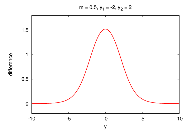
Since we want a configuration that at both spacial infinities, we can choose . Then at . Several numerical solutions are displayed in Fig. 5.


From Fig. 5, we clearly see that and for all the values of . As a position-dependent gauge coupling, we can choose a two-parameter family of desirable models
| (4.11) |
where can be any non-negative real numbers. This class of models can be easily made to localize non-Abelian gauge fields and minimally interacting matter fields by extending two of the factor groups to (possibly different) gauge groups with scalar fields in the fundamental representations, similarly to our model in previous sections. A new interesting feature of the four-flavor model (and its non-Abelian extensions) is that two possible profile of singlet fields can provide a different profile for different non-Abelian gauge groups such as , and with their associated matter fields.
5 Conclusion and discussion
We have successfully stabilized gauge fields and matter fields that are localized on domain walls. The low-energy effective Lagrangian on the domain wall has been worked out, where the adjoint matter fields is found to couple more strongly than singlet matter fields. We also explored possible generalization of our stabilization mechanism by including more fields and more gauge symmetries and found a class of more generic models with an added flexibility for model building with different localization profile for different gauge groups.
To build realistic models of brane-world with our scenario of localized gauge fields and matter fields, we should address several questions. Perhaps the most important question is to obtain (massless) matter fields in representations like the fundamental rather than the adjoint of localized gauge fields. One immediate possibility is to use the localization mechanism of fermions in a kink background. It has been found that zero modes of such fermions are localized in such a way to give automatically chiral fermions [21]. We will pursue this direction and associated anomaly questions further.
Secondly, we should devise a way to give small masses to our matter fields in order to do phenomenology. Since some of our matter fields are the Nambu-Goldstone modes of a broken global symmetry, we need to consider an explicit breaking of such global symmetry.
Thirdly, another question is to study possibility of supersymmetric model of gauge field localization. We need to settle the issues of possible new moduli in that case. Moreover, we should examine the mechanism of supersymmetry breaking.
Another interesting possibility for model building is to localize gauge fields of different gauge groups with different profiles. This situation is often proposed in recent brane-world phenomenology, for instance in Ref.[22].
Finally, let us examine similarities and differences of our domain walls compared to D-branes. The most interesting similarity of our domain wall with D-branes is the realization of geometrical Higgs mechanism, where massless gauge fields in the coincident wall become massive as walls separate. Detailed analysis of this phenomenon is worth doing. On the other hand, there are differences as well. D-branes in string theory are defined by the Dirichlet condition for fundamental string attached to it, but no such condition is visible in our domain walls. Domain walls similar to ours have been constructed in Ref.[23], where a probe magnetic charge is placed in the bulk Higgs phase. The magnetic flux from the probe magnetic monopole is carried by a vortex which can end on the domain wall. They observed that this wall-string junction configuration resembles an open string ending on D-branes in string theory. However, this phenomenon is in theories with one dimension less, namely the world volume of domain walls has only dimensions (fundamental theory is in dimensions). In our model based on a theory in dimensions, monopole (codimension three) is a string-like soliton, and might possibly be a candidate of something similar to the fundamental string. It is worth pursueing a possibility of composite solitons consisting of domain walls and other solitons such as monopoles, in order to clarify more similarities of solitons with D-branes. Another interesting issue of the effective action on D-branes is the non-Abelian generalization of the Dirac-Born-Infeld (DBI) action. There have been studies to obtain first few corrections to Yang-Mills action in string theories. Since we are at present interested in up to quadratic terms in derivatives, we have found the ordinary quadratic action of Yang-Mills fields together with the action of moduli fields interacting minimally with the Yang-Mills fields in addition to the nonlinear interactions among themselves. Our result is trivially consistent with the quadratic approximation of DBI action, but does not give us informations on non-Abelian generalization of DBI action. In order to shed lights on that issue, we need to compute higher derivative corrections to our effective Lagrangian, which is an interesting future problem.
Acknowledgements
This work is supported in part by Japan Society for the Promotion of Science (JSPS) and Academy of Sciences of the Czech Republic (ASCR) under the Japan - Czech Republic Research Cooperative Program, and by Grant-in-Aid for Scientific Research from the Ministry of Education, Culture, Sports, Science and Technology, Japan No.21540279 (N.S.), No.21244036 (N.S.), and No.23740226 (M.E.). The work of M.A. and F.B. is supported in part by the Research Program MSM6840770029 and by the project of International Cooperation ATLAS-CERN of the Ministry of Education, Youth and Sports of the Czech Republic.
Appendix A Derivation of the effective Lagrangian
In this appendix, we derive the effective Lagrangians (3.4) and (3.16) in the strong coupling limit. Since we are interested in the low energy effective Lagrangian, we focus on up the quadratic terms in derivatives, which we call .
A.1 Eliminating gauge fields
Here we eliminate gauge fields to obtain a nonlinear sigma model. Starting with in (2.42) in the strong gauge coupling limit and , is given as
| (A.1) |
where the covariant derivatives are given as:
| (A.2) |
Here we singled-out covariant derivatives containing fields associated with the gauged part of the flavor symmetry . Notice that and are no longer dynamical, but they are merely auxiliary fields to be eliminated. Moreover, the constraints are satisfied by the scalar fields (2.33)-(2.35) which depend on the moduli fields and
| (A.3) | ||||
| (A.4) |
The equation of motion for gives
| (A.5) |
where the sum over the index is implied (Einstein summation convention). Plugging this back into (A.1) we obtain
| (A.6) |
Next step is to eliminate the auxiliary fields . By using the following identities derived from the constraint (A.3)
| (A.7) | ||||
| (A.8) |
and by solving equations of motion for , we obtain
| (A.9) |
By using the following identities
| (A.10) |
where and , and
| (A.11) |
we obtain a simpler expression for
| (A.12) |
Using (A.12), we can rewrite the effective Lagrangian as an integral of a nonlinear sigma model over
| (A.13) |
A.2 Effective Lagrangian for and
Let us now calculate the effective Lagrangian including only fluctuations and around the coincident domain wall solutions (3.1)-(3.3) with (2.31) and (2.32). The composite fields are given as ()
| (A.14) | ||||
| (A.15) | ||||
| (A.16) |
After some algebra, covariant derivatives of these can be rewritten as
| (A.17) | ||||
| (A.18) | ||||
| (A.19) |
where
| (A.20) |
Putting this into Eq. (A.12) we obtain:
| (A.21) |
Substituting this result into (A.13), we obtain
| (A.22) |
Finally integration over is most easily done by substituting and using the identity:
| (A.23) |
leading to Eq.(3.4) (including the kinetic term for the gauge fields).
A.3 Effective Lagrangian for all terms: , and
Next we derive the effective Lagrangian including all fluctuations. Plugging the solution (3.11)-(3.13) into the Lagrangian (A.13), we obtain
| (A.24) |
where
| (A.25) |
| (A.26) |
| (A.27) |
and
| (A.28) |
The only work which remains to be done is to perform the integration. This, however, turns out to be difficult. The main source of difficulty lies in the fact the we cannot solve (3.15) explicitly. We therefore use some approximation technique, such as the Taylor expansion. We find it convenient to use as an expansion parameter which determines the width of the coincident wall. In the lowest order of approximation we see that Eq.(3.15) reduces to and we obtain the effective Lagrangian in Eq.(3.16).
A.4 Complexity of the Effective Lagrangian
The formula (3.16) illustrates the complexity of the interactions between moduli fields and in the general case. Let us offer some explanation for this complexity. The structure, which is new in (3.16) compared to (3.17) is of the general form
| (A.29) |
where and are some matrix-valued functions, containing either derivatives of or derivatives of . If we assume that is diagonalizable we can rewrite the above as
| (A.30) |
This form suggests that interaction (here represented by function ) depends on the relative size of fluctuation of each pairs of walls. Indeed, notice that if two walls have the same position (meaning that the expectation values of the fluctuations is the same), the above form reduces to
| (A.31) |
which is in a sense trivial, since we already encountered this kind of terms in (3.4). Thus, the new kind of complexity in our result (3.16) can be understood as a manifestation of the fact, that the interaction does not depend only on various moments of the fluctuation as in (3.17) but also on their relative size.
Appendix B Geometry of the three-flavor model
Quantum numbers of three-flavor model are shown in Tab. 5.
| mass | |||
|---|---|---|---|
| 1 | 0 | ||
| 1 | |||
| 0 | |||
| 0 | 0 | 0 | |
| 0 | 0 | 0 |
Since we are interested in the domain wall solutions, it is enough to consider the strong gauge coupling limit where gauge theories become non-linear sigma models (NLSM), whose target space is defined as an intersection of two spaces as
| (B.1) |
Here stands for the two dimensional hyperbolic plane. In the above expression, The and are defined by
| (B.2) | |||
| (B.3) |
This space is isomorphic to but it is a squashed sphere. The metric can be read from the Kähler potential
| (B.4) |
One can eliminate the real superfields and , and find the following expression of the Kähler potential with respect to the gauge invariant inhomogeneous coordinate as
| (B.5) | |||||
| (B.6) | |||||
| (B.7) |
Note that this manifold is singular at when . This can be understood in two different ways. The first one is to realize the fact that gauge symmetry is restored at that point. This is because holds there. Namely, the additional massless degrees of freedom should be taken into account. The second way is more straightforward. Let us calculate the scalar curvature in the vicinity of . To this end, first we change the coordinate by (), then we obtain
| (B.8) |
From this it is clear that the scalar curvature at becomes infinity when .
References
- [1] S. L. Dubovsky and V. A. Rubakov, Int. J. Mod. Phys. A 16 (2001) 4331 [hep-th/0105243].
- [2] G. R. Dvali and M. A. Shifman, Phys. Lett. B 396 (1997) 64 [Erratum-ibid. B 407 (1997) 452] [hep-th/9612128].
- [3] I. Antoniadis, N. Arkani-Hamed, S. Dimopoulos and G. R. Dvali, Phys. Lett. B 436 (1998) 257 [arXiv:hep-ph/9804398].
- [4] N. Maru and N. Sakai, Prog. Theor. Phys. 111 (2004) 907 [arXiv:hep-th/0305222].
- [5] J. B. Kogut and L. Susskind, Phys. Rev. D 9 (1974) 3501.
- [6] R. Fukuda, Phys. Lett. B 73 (1978) 305 [Erratum-ibid. B 74 (1978) 433];Mod. Phys. Lett. A 24 (2009) 251;arXiv:0805.3864 [hep-th].
- [7] H. Kawai and T. Kuroki, Phys. Lett. B 518 (2001) 294 [hep-th/0106103].
- [8] N. Seiberg, Phys. Lett. B 388 (1996) 753 [hep-th/9608111]; D. R. Morrison and N. Seiberg, Nucl. Phys. B 483 (1997) 229 [hep-th/9609070].
- [9] K. Ohta and N. Sakai, Prog. Theor. Phys. 124 (2010) 71 [Erratum-ibid. 127 (2012) 1133] [arXiv:1004.4078 [hep-th]].
- [10] M. Arai, F. Blaschke, M. Eto and N. Sakai, PTEP 2013 (2013) 013B05, [arXiv:1208.6219 [hep-th]].
- [11] M. Arai, F. Blaschke, M. Eto and N. Sakai, J. Phys. Conf. Ser. 411 (2013) 012001 [arXiv:1211.1235 [hep-th]].
- [12] M. Shifman and A. Yung, Phys. Rev. D 70 (2004) 025013 [hep-th/0312257].
- [13] M. Eto, M. Nitta, K. Ohashi and D. Tong, Phys. Rev. Lett. 95 (2005) 252003 [hep-th/0508130].
- [14] M. Eto, T. Fujimori, M. Nitta, K. Ohashi and N. Sakai, Phys. Rev. D 77 (2008) 125008 [arXiv:0802.3135 [hep-th]].
- [15] M. Eto, Y. Isozumi, M. Nitta, K. Ohashi and N. Sakai, Phys. Rev. D 73 (2006) 125008 [hep-th/0602289].
- [16] Y. Isozumi, M. Nitta, K. Ohashi and N. Sakai, Phys. Rev. Lett. 93 (2004) 161601 [arXiv:hep-th/0404198].
- [17] Y. Isozumi, M. Nitta, K. Ohashi and N. Sakai, Phys. Rev. D 70 (2004) 125014 [arXiv:hep-th/0405194].
- [18] M. Eto, Y. Isozumi, M. Nitta, K. Ohashi and N. Sakai, J. Phys. A A 39 (2006) R315 [hep-th/0602170].
- [19] N. S. Manton, Phys. Lett. B 110 (1982) 54; N. S. Manton and P. Sutcliffe, Topological Solitons (Cambridge Univiversity Press, Cambridge, England, 2004).
- [20] M. Eto, Y. Isozumi, M. Nitta, K. Ohashi, K. Ohta, N. Sakai and Y. Tachikawa, Phys. Rev. D 71 (2005) 105009 [hep-th/0503033].
- [21] V. A. Rubakov and M. E. Shaposhnikov, Phys. Lett. B 125 (1983) 136.
- [22] Y. Hosotani and Y. Kobayashi, Phys. Lett. B 674 (2009) 192 [arXiv:0812.4782 [hep-ph]].
- [23] M. Shifman and A. Yung, Phys. Rev. D 67 (2003) 125007 [hep-th/0212293].