跳到论文正文
W Papers独立论文阅读器 arXiv:1303.5127 论文正文 计算阅读时间 · 0%
引用这篇论文根据当前论文元数据生成,正式投稿前建议核对。


License: arXiv.org perpetual non-exclusive license
arXiv:1303.5127v1 [math.OC] 20 Mar 2013

Target-point based path following controller for a car-type vehicle using bounded controls

Salah Laghrouche* Affiliation: *SET Laboratory, UTBM, Belfort, France.    Mohamed Harmouche* Affiliation: **L2S, Université Paris-Sud 11, CNRS, Gif-sur-Yvette, France.    Yacine Chitour** Affiliation: mohamed.harmouche@utbm.fr, salah.laghrouche@utbm.fr, yacine.chitour@lss.supelec.fr

Abstract

In this paper, we have studied the control problem of target-point based path following for car-type vehicles. This special path following task arises from the needs of vision based guidance systems, where a given target-point located ahead of the vehicle, in the visual range of the camera, must follow a specified path. A solution to this problem is developed through a non linear transformation of the path following problem into a reference trajectory tracking problem, by modeling the target point as a virtual vehicle. Bounded feedback laws must be then used on the real vehicle’s angular acceleration and the virtual vehicle’s velocity, to achieve stability. The resulting controller is globally asymptotically stable with respect and the proof is demonstrated using Lyapunov based arguments and a bootstrap argument. The effectiveness of this controller has been illustrated through simulations.

I Introduction

In the field of autonomous vehicle guidance, navigation and control, path-following problem of car-type vehicles is of particular interest. Many contemporary researchers have published various techniques and strategies for this problem, such as [1, 2, 3, 4, 5, 6]. Among open-loop motion planning techniques, differential flatness approach has been significant in motion planning to drive vehicles on Cartesian paths [7, 8]. In feedback control techniques, larger effort has been made on tracking problems. A backstepping approach has been presented in the context of tracking in [9]. This approach has also been used in [10], to develop a controller that is robust against vehicle skidding effects. Do et al. have further improved upon Jiang’s backstepping method in [11] and [12], by adding observers to render the controller output-feedback and extending it to tracking and stabilization for parking problems of a vehicle and introducing dynamic update laws to compensate for parametric uncertainty and modeling errors. In [13] Aguiar et al. have used adaptive switched supervisory control combined with a non linear Lyapunov-based control to ensure the global convergence of the position tracking error to a small neighborhood of the origin. Bloch and Drakunov [14] have used sliding mode control for the stabilization and tracking of a nonholonomic dynamic system. This controller is global and ensures convergence to the neighborhood of the desired trajectory. Lee et al. [15] have proposed a saturated feedback controller for tracking of a unicycle-type vehicle, using its forward velocity and angular acceleration as control inputs. They have also extended this controller for application on car-type vehicles.

The problem of path following differs from pure stabilization or tracking problems because the path, described by its curvature κ(.)\displaystyle\kappa(.), is defined in space only, not in time. In this paper, we have addressed the path following control of a robot car-type vehicle using target point. This control problem arises from camera-vision applications [16, 17], where the vehicle is guided by a target point ahead of the vehicle, within the visual range of the camera [18, 16]. The target point is fixed at a known distance d>0\displaystyle d>0 from the center of gravity on the axis of the vehicle. The control objective is to drive the vehicle, such that the target point follows the desired path (as shown in Fig. 1). This problem has been addressed in [19] where a local robust path following strategy has been proposed using target point. Their solution is based on an open loop control based on inversion of the nominal model, and a closed loop control for stabilization of the resultant system. The error dynamics have been expressed in the Frénet frame associated to the followed path. This technique, also discussed in [20], is convenient only when the vehicle is close, positioned and oriented to the path.

In our work, a global asymptotically stable controller is developed by parameterizing the path as a “virtual vehicle”, which is tracked by the actual vehicle. In this way, the path following problem is converted into a tracking problem, with two control inputs: the angular acceleration of the real vehicle and the velocity of the virtual vehicle. The forward velocity control of the real vehicle is not considered as part of the navigation problem, as it is controlled by other intelligent control systems in practical applications (for example, ABS, ESP [21]). It is instead assumed to be a measured state that is strictly positive, meaning that the vehicle is in continuous forward motion.

It can be noted that if there is no target point, i.e. d=0\displaystyle d=0, then the tracking error model obtained in this study is identical to [15], in which tracking has been achieved by using saturation on one control input while the other is unbounded. In our case, the introduction of the target point at a distance makes the dynamics of the tracking error model more complicated. Specifically, the development produces a first order nonlinear non-globally Lipschitz differential equation (see equation (21)) that can blow up in finite time. To overcome this difficulty, our solution necessitates the application of saturated controls for both our control inputs with arbitrary small amplitude. Examples of application of saturated control can be found in [22, 23, 24, 25, 26, 27]. Consequently, if both the control inputs are applied on the real vehicle, then the path following problem developed here becomes equivalent to the generalization of [15], as tracking problem with a target-point.

This paper can be seen as the continuation of the authors’ previous work in [28], in which a unicycle type vehicle had been considered. However, the arguments of the Lyapunov analysis used for the convergence proof are significantly more involved than that of [28], due to the added state of the car type vehicle (essentially an integrator) and the fact that one must keep track of the small amplitudes of the saturations. Therefore, a positive definite function V\displaystyle V is designed instead of a global Lyapunov function, whose time derivative along the closed-loop system is strictly negative outside a neighborhood of the origin. The design of V\displaystyle V relies on an asymptotic analysis of a Ricatti equation, which is not needed in [28]. The convergence to zero is then demonstrated using a bootstrap procedure [29], i.e., once the system errors converge to a neighborhood, they continue to diminish to a smaller neighborhood, and ultimately converge asymptotically to the origin. The results so obtained can be extended to the case where only the position of the reference trajectory is directly known.

The paper is organized as follows: in Section 2, the vehicle model and reference trajectory parameterization have been presented. In Section 3, the control design has been discussed and the Lyapunov function has been developed. The stability analysis of the closed loop system has been discussed in Section 4. Simulation results have been provided in Section 5, and a conclusion has been presented in Section 6.

II Vehicle model and reference trajectory

Let us consider a path Γ\displaystyle\Gamma with geodesic curvature κr\displaystyle\kappa_{r} whose absolute value is bounded by κm​a​x>0\displaystyle\kappa_{max}>0, i.e., for all t≥0\displaystyle t\geq 0, we have

|κr​(t)|≤κm​a​x.|\kappa_{r}(t)|\leq\kappa_{max}. (1)

As described in the introduction, Γ\displaystyle\Gamma will be parameterized as a vehicle trajectory with a forward velocity u⁡(t)\displaystyle u(t) such that Γ⁡(t)=(pr​(t),qr​(t))\displaystyle\Gamma(t)=(p_{r}(t),q_{r}(t)) is described by the following state equations

{p˙r=ucosψr,q˙r=usinψr,ψ˙r=u​κr,κ˙r=u​ρr,\displaystyle\displaystyle\left\{\begin{array}[]{rcl}\dot{p}_{r}&=&u\ \cos{\psi_{r}},\\ \dot{q}_{r}&=&u\ \sin{\psi_{r}},\\ \dot{\psi}_{r}&=&u\ \kappa_{r},\\ \dot{\kappa}_{r}&=&u\ \rho_{r},\end{array}\right.

where ψr\displaystyle\psi_{r} represents the angle between the abscissa axis and the velocity vector (p˙r,q˙r)T\displaystyle(\dot{p}_{r},\dot{q}_{r})^{T}, and κr\displaystyle\kappa_{r} is the scalar curvature associated to the parametrization of Γ\displaystyle\Gamma by time t\displaystyle t. The arclength s\displaystyle s of Γ\displaystyle\Gamma is given by s⁡(t)=s0+∫0tu⁡(τ)​𝑑τ\displaystyle s(t)=s_{0}+\int_{0}^{t}u(\tau)d\tau and the scalar curvature κr​(t)\displaystyle\kappa_{r}(t) is hence equal to κr∗​(s⁡(t))\displaystyle\kappa_{r}^{*}(s(t)).

The state equations for the vehicle dynamics are

{x˙=Vx​cos⁡ψ,y˙=Vx​sin⁡ψ,ψ˙=Vx​κ,κ˙=Vx​ρ0.\displaystyle\displaystyle\left\{\begin{array}[]{rcl}\dot{x}&=&V_{x}\ \cos{\psi},\\ \dot{y}&=&V_{x}\ \sin{\psi},\\ \dot{\psi}&=&V_{x}\ \kappa,\\ \dot{\kappa}&=&V_{x}\ \rho_{0}.\end{array}\right.

These equations represent the vehicle’s motion with a velocity Vx\displaystyle V_{x}, along the curve defined by the its geodesic curvature κ\displaystyle\kappa. The control variable ρ0\displaystyle\rho_{0} will be defined later. Notice that Vx\displaystyle V_{x} is not necessarily constant, but simply a continuous function of time, which verifies the following hypothesis: there exist two positive constants 0<Vm​i​n≤Vm​a​x\displaystyle 0<V_{min}\leq V_{max}, such that for all t≥0\displaystyle t\geq 0

Vm​i​n≤Vx​(t)≤Vm​a​x.V_{min}\leq V_{x}(t)\leq V_{max}. (12)

The strict positivity of the lower bound is necessary to derive our subsequent results. Note that path following for a unicycle type of vehicle has been obtained under weaker hypotheses than that of the above equation, cf. in particular the persistent excitation condition (PEC) [30]. It is not clear to us how to extend the present work only assuming that Vx\displaystyle V_{x} satisfies the PEC (see Remark (III.1)).

For the target point, the equations for the coordinates p\displaystyle p and q\displaystyle q are defined as

p=x+d​cos⁡ψ,q=y+d​sin⁡ψ.\displaystyle\displaystyle\begin{array}[]{rcl}p&=x+d\cos{\psi},\\ q&=y+d\sin{\psi}.\\ \end{array}

We will also suppose throughout the paper that

  • (H1)

    d​κm​a​x<1\displaystyle d\kappa_{max}<1.

Remark II.1.

The above assumption may be considered as a technical one or a design constraint for positioning the target point. However, it is reasonable to upper bound the curvature of the reference path in terms of the distance d\displaystyle d. Indeed, tracking a circle of radius d′<d\displaystyle d^{\prime}<d with a point fixed at a distance d\displaystyle d in front of a vehicle is impossible. To see that, one can see that intuitively of rely on equation (160) given below. At the ligth of the previous example, Hypothesis (H​1)\displaystyle(H1) is almost optimal.

The dynamics of the target point in a form similar to (II) can be obtained by deriving the precedent equations. One first gets that

{p˙=Vx​cos⁡ψ−d​Vx​sin⁡ψ​κ,q˙=Vx​sin⁡ψ+d​Vx​cos⁡ψ​κ,\displaystyle\displaystyle\left\{\begin{array}[]{rcl}\dot{p}&=&V_{x}\ \cos{\psi}-d\ V_{x}\ \sin{\psi}\ \kappa,\\ \dot{q}&=&V_{x}\ \sin{\psi}+d\ V_{x}\ \cos{\psi}\ \kappa,\\ \end{array}\right.
Refer to caption
Fig. 1: The reference trajectory, the vehicle and its target point.

The curve defined by the target point is traveled at the following speed

vd=p˙2+q˙2=Vx​1+(κ​d)2.v_{d}=\sqrt{\dot{p}^{2}+\dot{q}^{2}}=V_{x}\sqrt{1+(\kappa d)^{2}}. (19)

Our objective now is to define the dynamics of the target point as those of a car. For that purpose, we consider θ\displaystyle\theta as the angle between the abscissa axis and the velocity vector (p˙,q˙)T\displaystyle(\dot{p},\dot{q})^{T}. One easily gets that

θ=ψ+arctan⁡(κ​d),\theta=\psi+\arctan(\kappa d), (20)

then p˙=vd​cos⁡(θ),q˙=vd​sin⁡(θ)\displaystyle\dot{p}=v_{d}\cos(\theta),\ \ \ \dot{q}=v_{d}\sin(\theta), and the scalar curvature ω\displaystyle\omega is defined by ω=θ˙vd\displaystyle{\displaystyle\omega=\frac{\dot{\theta}}{v_{d}}}.

We define the dynamics of ω\displaystyle\omega by the new control variable ρ:=ω˙/vd\displaystyle\rho:=\dot{\omega}/v_{d}\ . Deriving equation (20), we obtain

d​κ˙=Vx​(1+(κ​d)2)​((1+(κ​d)2)1/2​ω−κ).d\dot{\kappa}=V_{x}(1+(\kappa d)^{2})((1+(\kappa d)^{2})^{1/2}\omega-\kappa). (21)

Hence the dynamics of the target point (p,q)\displaystyle(p,q) becomes

{p˙=vd​cos⁡θ,q˙=vd​sin⁡θ,θ˙=vd​ω,ω˙=vd​ρ.\displaystyle\displaystyle\left\{\begin{array}[]{rcl}\dot{p}&=&v_{d}\ \cos{\theta},\\ \dot{q}&=&v_{d}\ \sin{\theta},\\ \dot{\theta}&=&v_{d}\ \omega,\\ \dot{\omega}&=&v_{d}\ \rho.\end{array}\right.

The error between the target point and the reference curve is defined as

ep=p−pr,eq=q−qr,ξ=θ−ψr,η=ω−κr.\displaystyle\displaystyle\begin{array}[]{rcl}e_{p}&=&p-p_{r},\\ e_{q}&=&q-q_{r},\\ \xi&=&\theta-\psi_{r},\\ \eta&=&\omega-\kappa_{r}.\end{array}

and the error dynamics is given by

{e˙p=vdcosθ−ucosψr,e˙q=vdsinθ−usinψr,ξ˙=vd​ω−κr​u,η˙=vd​ρ−ρr​u.\displaystyle\displaystyle\left\{\begin{array}[]{rcl}\dot{e}_{p}&=&v_{d}\ \cos{\theta}-u\cos{\psi_{r}},\\ \dot{e}_{q}&=&v_{d}\ \sin{\theta}-u\sin{\psi_{r}},\\ \dot{\xi}&=&v_{d}\ \omega-\kappa_{r}\ u,\\ \dot{\eta}&=&v_{d}\ \rho-\rho_{r}\ u.\end{array}\right.

III Control design and Lyapunov Function

In this section, we will present a control law u⁡(ep,eq,ξ,η,t)\displaystyle u(e_{p},e_{q},\xi,\eta,t) and ρ⁡(ep,eq,ξ,η,t)\displaystyle\rho(e_{p},e_{q},\xi,\eta,t), such that the system (II) is globally asymptotically stable (GAS for short) w.r.t. origin. Note that, from the equations (19) and (21), one recovers the control ρ0\displaystyle\rho_{0} once vd\displaystyle v_{d} and ρ\displaystyle\rho are determined. However, there is an issue of possible blow-up in finite time for κ\displaystyle\kappa (and thus for ρ0\displaystyle\rho_{0}). Indeed, assuming that one is able to stabilize (II) to zero, then the control ρ0\displaystyle\rho_{0} is obtained by derivating κ\displaystyle\kappa, which is in turn obtained by solving (21), seen as an o.d.e. with unknown κ\displaystyle\kappa since ω\displaystyle\omega tends to κr\displaystyle\kappa_{r} asymptotically. Equation (21) is of the type κ˙=f⁡(κ,t)\displaystyle\dot{\kappa}=f(\kappa,t) with the right-hand side f\displaystyle f not globally Lipschitz w.r.t. κ\displaystyle\kappa, hence it is not immediate to insure global existence of κ\displaystyle\kappa for all t≥0\displaystyle t\geq 0. We will show later on, that an appropriate choice of u\displaystyle u and ρ\displaystyle\rho under Hypothesis (H1) solves this problem (see Lemma IV.1 below).

The standard saturation function σ⁡(x)\displaystyle\sigma(x) defined for x∈ℝ\displaystyle x\in\mathbb{R} by

σ⁡(x)=xmax⁡(1,|x|).\sigma(x)=\frac{x}{\max(1,|x|)}. (37)

Let us first of all perform a variable change on the control, as follows

u=vd​(1+u1),ρ=ρr​(1+u1)+u2,\displaystyle\displaystyle\begin{array}[]{rcl}u&=&v_{d}(1+u_{1}),\\ \rho&=&\rho_{r}(1+u_{1})+u_{2},\end{array}

where u1,u2\displaystyle u_{1},\ u_{2} are the new control variables.

Remark III.1.

In order to define ω\displaystyle\omega, ρ\displaystyle\rho and to perform the change of inputs variables, vd\displaystyle v_{d} must be greater than zero and thus Vx\displaystyle V_{x} must also be strictly positive. It is therefore not obvious to proceed as above, if Vx\displaystyle V_{x} only satisfies (PEC).

With the boundedness of κ\displaystyle\kappa and Vx\displaystyle V_{x}, equation (19) implies that νd\displaystyle\nu_{d} is bounded. If one insists on having ρ\displaystyle\rho bounded, then we must assume also that ρr\displaystyle\rho_{r} is bounded, as

|ρr|≤ρr,m​a​x,\begin{array}[]{lcl}\left|\rho_{r}\right|\leq\rho_{r,max},\end{array} (41)

where ρr,m​a​x\displaystyle\rho_{r,max} is a known positive constant.

The system (II) is therefore rewritten as

{e˙p=vd(cosθ−cosψr−u1cosψr),e˙q=vd(sinθ−sinψr−u1sinψr),ξ˙=vd​(η−κr​u1),η˙=vd​u2.\displaystyle\displaystyle\left\{\begin{array}[]{rcl}\dot{e}_{p}&=&v_{d}(\cos{\theta}-\cos{\psi_{r}}-\ u_{1}\cos{\psi_{r}}),\\ \dot{e}_{q}&=&v_{d}(\sin{\theta}-\sin{\psi_{r}}-\ u_{1}\sin{\psi_{r}}),\\ \dot{\xi}&=&v_{d}(\eta-\kappa_{r}u_{1}),\\ \dot{\eta}&=&v_{d}u_{2}.\end{array}\right.

The bounded controls u1\displaystyle u_{1} and u2\displaystyle u_{2} can be expressed in the following form:

u1=C1​σ​(⋅),u2=D​σ​(⋅),\displaystyle\displaystyle\begin{array}[]{rcl}u_{1}&=&C_{1}\sigma(\cdot),\\ u_{2}&=&D\sigma(\cdot),\end{array}

with sufficiently small gains C1\displaystyle C_{1} and D\displaystyle D. Since κ\displaystyle\kappa is bounded, vd\displaystyle v_{d} also remains uniformly bounded throughout t≥0\displaystyle t\geq 0. We can hence change the time scale by considering d​s=vd​d​t\displaystyle ds=v_{d}\ dt. To keep the notations simple, we would continue to use t\displaystyle t for time, and the point for the derivation with respect to s\displaystyle s, like d​fd​s=f˙\displaystyle\frac{df}{ds}=\dot{f}. This has no effect on the control laws since our design is based on static feedback (w.r.t. the error). The error dynamics hence becomes

{e˙p=cosθ−cosψr−u1cosψr,e˙q=sinθ−sinψr−u1sinψr,ξ˙=η−κr​u1,η˙=u2.\displaystyle\displaystyle\left\{\begin{array}[]{rcl}\dot{e}_{p}&=&\cos{\theta}-\cos{\psi_{r}}-u_{1}\cos{\psi_{r}},\\ \dot{e}_{q}&=&\sin{\theta}-\sin{\psi_{r}}-u_{1}\sin{\psi_{r}},\\ \dot{\xi}&=&\eta-\kappa_{r}u_{1},\\ \dot{\eta}&=&u_{2}.\end{array}\right.

Let us perform the following change of variable corresponding to a time-varying rotation in the frame of the reference trajectory

y1=epcosψr+eqsinψr,y2=−epsinψr+eqcosψr.\displaystyle\displaystyle\begin{array}[]{rcl}y_{1}&=&e_{p}\ \cos{\psi_{r}}+e_{q}\ \sin{\psi_{r}},\\ y_{2}&=&-e_{p}\ \sin{\psi_{r}}+e_{q}\ \cos{\psi_{r}}.\end{array}

The system becomes

{y˙1=−u1+(cos⁡ξ−1)+(1+u1)​κr​y2,y˙2=sin⁡ξ−(1+u1)​κr​y1,ξ˙=η−κr​u1,η˙=u2,\displaystyle\displaystyle\left\{{\begin{array}[]{rcl}\dot{y}_{1}&=&-u_{1}+(\cos{\xi}-1)+(1+u_{1})\kappa_{r}y_{2},\\ \dot{y}_{2}&=&\sin{\xi}-(1+u_{1})\kappa_{r}y_{1},\\ \dot{\xi}&=&\eta-\kappa_{r}u_{1},\\ \dot{\eta}&=&u_{2},\end{array}}\right.

where u1\displaystyle u_{1}, u2\displaystyle u_{2} will be chosen such that (III) becomes GAS.
The control variables u1\displaystyle u_{1} and u2\displaystyle u_{2} are defined as follows

u1=C1​σ​(y1),u2=−D​σ​(k1D​ξ+k2D​η+C2D​σ​(y2)),\displaystyle\displaystyle\begin{array}[]{rcl}{u_{1}}&=&{C_{1}}\sigma(y_{1}),\\ {u_{2}}&=&-D\sigma(\frac{k_{1}}{D}\xi+\frac{k_{2}}{D}\eta+\frac{C_{2}}{D}\sigma(y_{2})),\hfill\\ \end{array}

where k1,k2,C1,C2,D\displaystyle k_{1},k_{2},C_{1},C_{2},D are positive real numbers and σ⁡()\displaystyle\sigma() is the standard saturation function defined in (37). Typically, we want to stabilize the system with arbitrarily small saturation levels C1\displaystyle C_{1} and D\displaystyle D. In conclusion, the final system, noted (Σ\displaystyle\Sigma) becomes

(Σ){y˙1=−C1​σ​(y1)+(cos⁡ξ−1)+μ​y2,y˙2=sin⁡ξ−μ​y1,ξ˙=η−κr​C1​σ​(y1),η˙=−D​σ​(k1D​ξ+k2D​η+C2D​σ​(y2)),\displaystyle\displaystyle(\Sigma)\quad\left\{{\begin{array}[]{rcl}\dot{y}_{1}&=&-{C_{1}}\sigma({{y_{1}}})+(\cos{\xi}-1)+\mu y_{2},\\ \dot{y}_{2}&=&\sin{\xi}-\mu y_{1},\\ \dot{\xi}&=&\eta-\kappa_{r}{C_{1}}\sigma({{y_{1}}}),\\ \dot{\eta}&=&-D\sigma(\frac{k_{1}}{D}\xi+\frac{k_{2}}{D}\eta+\frac{C_{2}}{D}\sigma(y_{2})),\end{array}}\right.

where

μ:=κr​(1+C1​σ​(y1))​ and ​|μ|≤κm​a​x​(1+C1).\mu:=\kappa_{r}(1+{C_{1}}\sigma({{y_{1}}}))\hbox{ and }|\mu|\leq\kappa_{max}(1+C_{1}). (71)

In the following section, it is shown that Global Asymptotic Stability of the system (III) can be achieved by proper selection of C1\displaystyle C_{1}, C2\displaystyle C_{2}, k1\displaystyle k_{1}, k2\displaystyle k_{2}.

More precisely, we prove the following theorem, which is the main result of the paper.

Theorem III.2.

Consider a path Γ\displaystyle\Gamma with geodesic curvature κr∗\displaystyle\kappa_{r}^{\ast} verifying (1) for some κm​a​x>0\displaystyle\kappa_{max}>0. It is then possible to track asymptotically γ\displaystyle\gamma with a point fixed at a distance d>0\displaystyle d>0 in front of a vehicle, where d​κm​a​x<1\displaystyle d\kappa_{max}<1, by choosing the control laws u1,u2\displaystyle u_{1},u_{2} according to (III) with constants k1,k2,C1,C2,D\displaystyle k_{1},k_{2},C_{1},C_{2},D, which satisfy the following conditions. Set a:=316\displaystyle a:=\frac{3}{16}.

k1=a​k22,C2=12​β​k2,C1=a​C24​k2,k_{1}=a{k_{2}}^{2},\ C_{2}=\frac{1}{2\beta k_{2}},\ C_{1}=\frac{aC_{2}}{4k_{2}}, (72)

where β\displaystyle\beta is a positive constant larger than 8\displaystyle 8, D\displaystyle D is an arbitrary positive constant, fixed a-priori, and k2\displaystyle k_{2} is large enough that 1k2​D≪1\displaystyle\frac{1}{k_{2}D}\ll 1.

Proof.

The proof of GAS stability of System (III) has been carried out as an argument based on Lyapunov analysis.

The first remark consists in focusing on the last two equations in (Σ)\displaystyle(\Sigma) and we will first treat the case where there is no saturation on η˙\displaystyle\dot{\eta}.

In that case, the last two equations in the previous section define a double integrator system, which shall now be denoted as (Sk\displaystyle S_{k}):

(Sk){ξ˙=η+v1,η˙=−k1​ξ−k2​η+v2,\displaystyle\displaystyle\begin{array}[]{rcl}(S_{k})\quad\left\{\begin{gathered}\dot{\xi}=\eta+{v_{1}},\hfill\\ \dot{\eta}=-{k_{1}}\xi-{k_{2}}\eta+{v_{2}},\hfill\\ \end{gathered}\right.\end{array}

with,

v1=−κr​C1​σ​(y1),v2=−C2​σ​(y2).\displaystyle\displaystyle\begin{array}[]{rcl}\begin{gathered}{v_{1}}=-{\kappa_{r}}{C_{1}}\sigma\left({{y_{1}}}\right),\hfill\\ {v_{2}}=-{C_{2}}\sigma({y_{2}}).\hfill\\ \end{gathered}\end{array}

The system (Sk)\displaystyle(S_{k}) can be presented in the matrix form

Z˙=A​Z+B​U,\displaystyle\displaystyle\begin{array}[]{rcl}\dot{Z}=AZ+BU,\end{array}

where,

Z=(ξη),A=(01−k1−k2),B=(1001),U=(ν1ν2).\displaystyle\displaystyle\begin{array}[]{l}Z=\left(\begin{array}[]{l}\xi\\ \eta\\ \end{array}\right),\ A=\left({\begin{array}[]{*{20}{c}}0&1\\ {-{k_{1}}}&{-{k_{2}}}\\ \end{array}}\right),\ B=\left({\begin{array}[]{*{20}{c}}1&0\\ 0&1\\ \end{array}}\right),\ U=\left(\begin{array}[]{l}{\nu_{1}}\\ {\nu_{2}}\\ \end{array}\right).\\ \end{array}

Since A\displaystyle A is Hurwitz, there exists a quadratic form Vk=ZT​Pk​Z\displaystyle V_{k}=Z^{T}P_{k}Z, where Pk\displaystyle P_{k} is a positive definite square matrix, obtained by solving the following Riccati equation

Pk​A+AT​Pk+Pk2ΥL2=−I,\displaystyle\displaystyle\begin{array}[]{rcl}{P_{k}}A+{A^{T}}{P_{k}}+\frac{P_{k}^{2}}{\Upsilon_{L}^{2}}=-I,\end{array}

where, ΥL\displaystyle\Upsilon_{L} is the L2\displaystyle L_{2}-gain related to the system (Sk)\displaystyle(S_{k}). The derivative V˙k\displaystyle\dot{V}_{k} is given by the following equation

V˙k=−‖Z‖2−‖Pk​Z‖2ΥL2+2​ZT​Pk​U,\displaystyle\displaystyle\begin{array}[]{rcl}{{\dot{V}}_{k}}=-{\left\|Z\right\|^{2}}-\frac{{{{\left\|{P_{k}}Z\right\|}^{2}}}}{{\Upsilon_{L}^{2}}}+2{Z^{T}}{P_{k}}U,\end{array}

and verifies

V˙k≤−‖Z‖2+ΥL2​‖U‖2.\displaystyle\displaystyle\begin{array}[]{rcl}{{\dot{V}}_{k}}\leq-{\left\|Z\right\|^{2}}+\Upsilon_{L}^{2}{\left\|U\right\|^{2}}.\end{array}

The Lyapunov function proposed for the global system (III) is

V=M​Vk+k1​y12+y222+η​y2+k2​y2​ξ,\displaystyle\displaystyle\begin{array}[]{rcl}V&=&M{V_{k}}+{k_{1}}\frac{{y_{1}^{2}+y_{2}^{2}}}{2}+\eta{y_{2}}+{k_{2}}{y_{2}}\xi,\\ \end{array}

where M,k1,k2\displaystyle M,\ k_{1},\ k_{2} are positive constants to be chosen later in particular to ensure that V is positive definite function, see Lemma III.6 below. Moreover, a straightforward computation yields the following:

Proposition III.3.

The derivative of the Lyapunov function can be upper bounded as follows,

V˙≤−M⁡(ξ2+η2)−k1​C1​y1​σ​(y1)−C2​y2​σ​(y2)+M​ΥL2​((κr​C1​σ​(y1))2+(C2​σ​(y2))2)+k1​y2​(sin⁡ξ−ξ)+k1​y1​(cos⁡ξ−1)−μ​η​y1+η​sin⁡ξ−k2​y2​κr​C1​σ​(y1)−k2​ξ​μ​y1+k2​ξ​sin⁡ξ.\displaystyle\displaystyle\begin{array}[]{rcl}\begin{gathered}\begin{array}[]{rcl}\dot{V}&\leq&-M({\xi^{2}+\eta^{2}})-{k_{1}}{C_{1}}{y_{1}}\sigma\left({{y_{1}}}\right)-{C_{2}y_{2}}\sigma\left({{y_{2}}}\right)+M{\Upsilon_{L}}^{2}\left({{{\left({{\kappa_{r}}C_{1}\sigma\left({{y_{1}}}\right)}\right)}^{2}}+({C_{2}\sigma\left({{y_{2}}}\right)})^{2}}\right)\\ &&+k_{1}y_{2}(\sin\xi-\xi)+k_{1}y_{1}(\cos\xi-1)-\mu\eta{y_{1}}+\eta\sin\xi-{k_{2}}{y_{2}}{\kappa_{r}}{C_{1}}\sigma\left({{y_{1}}}\right)-{k_{2}}\xi\mu{y_{1}}+{k_{2}}\xi\sin\xi.\\ \end{array}\end{gathered}\end{array}

The rest of the argument is divided in two main steps. In the first step, the existence of appropriate constants M,k1,k2,C1,C2\displaystyle M,k_{1},k_{2},C_{1},C_{2} is proven, such that V\displaystyle V has a positive definite quadratic form in all the variables. This means that there exists a bounded region Yk2\displaystyle Y_{k_{2}} (for k2\displaystyle k_{2} typically large), in the (y1,y2)−\displaystyle(y_{1},y_{2})-plane:

Yk2={(y1,y2)||y1|≤Ck22,|y2|≤Ck23/2},Y_{k_{2}}=\{(y_{1},y_{2})|\quad|y_{1}|\leq\frac{C}{k_{2}^{2}},\ |y_{2}|\leq\frac{C}{k_{2}^{3/2}}\}, (108)

such that outside this region, the derivative of V\displaystyle V along trajectories of (III) fulfills the following inequality

V˙≤−M2​(ξ2+η2)−k1​C12​y1​σ​(y1)−C22​y2​σ​(y2).\dot{V}\leq-\frac{M}{2}({\xi^{2}+\eta^{2}})-{k_{1}}\frac{C_{1}}{2}{y_{1}}\sigma\left({{y_{1}}}\right)-\frac{C_{2}}{2}{y_{2}}\sigma\left({{y_{2}}}\right). (109)

In the second step, a bootstrap-type argument is applied to show the convergence of trajectories of (III) to zero, as t\displaystyle t tends to infinity.

These two steps have been achieved in the following manner: the L2\displaystyle L_{2}-gain of (Sk)\displaystyle(S_{k}), denoted by ΥL\displaystyle\Upsilon_{L} is calculated, then Pk\displaystyle P_{k} is estimated for k2\displaystyle k_{2} tending to infinity. Then ISS (input-to-state) type bounds are calculated for ξ\displaystyle\xi and η\displaystyle\eta and the derivative of the Lyapunov function is estimated outside Yk2\displaystyle Y_{k_{2}}, and the argument is concluded. The detailed calculations have been presented in the following subsections.

III-A L2\displaystyle L_{2}-gain ΥL\displaystyle\Upsilon_{L}

Let us study the system (Sk\displaystyle S_{k}), defined in the equation (III). We recall that, (Sk\displaystyle S_{k}) can be presented in the following matrix form

(ξ˙η˙)⏟Z˙=(01−k1−k2)⏟A​(ξη)⏟Z+(1001)⏟B​(v1v2).⏟U\displaystyle\displaystyle\begin{array}[]{rcl}\underbrace{\left({\begin{array}[]{*{20}{c}}{\dot{\xi}}\\ {\dot{\eta}}\\ \end{array}}\right)}_{\dot{Z}}=\underbrace{\left({\begin{array}[]{*{20}{c}}0&1\\ {-{k_{1}}}&{-{k_{2}}}\\ \end{array}}\right)}_{A}\underbrace{\left({\begin{array}[]{*{20}{c}}\xi\\ \eta\\ \end{array}}\right)}_{Z}+\underbrace{\left({\begin{array}[]{*{20}{c}}1&0\\ 0&1\\ \end{array}}\right)}_{B}\underbrace{\left({\begin{array}[]{*{20}{c}}{{v_{1}}}\\ {{v_{2}}}\\ \end{array}}\right).}_{U}\end{array}
Lemma III.4.

We will tune k2≥20\displaystyle k_{2}\geq 20 with k1=316​k22\displaystyle k_{1}=\frac{3}{{16}}k_{2}^{2}, then 1<ΥL<1.2\displaystyle 1<\Upsilon_{L}<1.2.

The proof of Lemma III.4 is given in Appendix.

III-B Estimation of Pk\displaystyle P_{k} for large k2\displaystyle k_{2}

In this section, we take k1=a​k22\displaystyle{k_{1}}=ak_{2}^{2} with a=316\displaystyle a=\frac{3}{{16}} and k2\displaystyle k_{2} tending to infinity. We will prove the following two results whose proofs are given in Appendix.

Lemma III.5.

As k2\displaystyle k_{2} tends to infinity, the positive define matrix Pk\displaystyle P_{k} defined in (III) admits the following asymptotic expansion

Pk=(p1​k2p2p2p3k2),P_{k}=\begin{pmatrix}p_{1}k_{2}&p_{2}\\ p_{2}&\frac{p_{3}}{k_{2}}\end{pmatrix}, (122)

with pi=Fi​(1+O⁡(1k22))\displaystyle p_{i}=F_{i}(1+O(\frac{1}{k_{2}^{2}})), 1≤i≤3\displaystyle 1\leq i\leq 3, where the Fi\displaystyle F_{i} are positive constants (only depending on a\displaystyle a) so that F1​F3−F22>0\displaystyle F_{1}F_{3}-F_{2}^{2}>0.

Proposition III.6.

For k2\displaystyle k_{2} large enough and M=β​k2\displaystyle M=\beta k_{2}, the function V\displaystyle V defined in (III) is a positive quadratic form in (ξ,η,y1,y2)\displaystyle(\xi,\eta,y_{1},y_{2}).

III-C ISS bounds for ξ\displaystyle\xi and η\displaystyle\eta

For a real-valued continuous and bounded function f\displaystyle f defined on ℝ+\displaystyle\mathbb{R}^{+}, we set

|f|∗​(t):=sups≥t|f⁡(s)|,|f|^{*}(t):=\sup_{s\geq t}|f(s)|,

and

‖f‖∗:=lim sups→∞|f⁡(s)|.\|f\|^{*}:=\limsup_{s\rightarrow\infty}|f(s)|.
Lemma III.7.

Consider the system (III-A). By tuning k1=316​k22\displaystyle{k_{1}}=\frac{3}{{16}}k_{2}^{2} , the ISS bounds of ξ\displaystyle\xi and η\displaystyle\eta satisfy the following inequalities for t≥0\displaystyle t\geq 0,

{|ξ|∗​(t)≤4k2​(κm​a​x​C1+43​k2​C2)+‖eA​t​Z0‖,|η|∗​(t)≤κm​a​x​C1+163​k2​C2+‖eA​t​Z0‖,\displaystyle\displaystyle\begin{array}[]{rcl}\begin{gathered}\left\{\begin{array}[]{l}{\begin{array}[]{*{20}{c}}|\xi|^{*}(t)\\ \end{array}}\leq\frac{4}{{{k_{2}}}}\left({\kappa_{max}{C_{1}}+\frac{4}{{3{k_{2}}}}{C_{2}}}\right)+\|e^{At}Z_{0}\|,\\ {\begin{array}[]{*{20}{c}}|\eta|^{*}(t)\\ \end{array}}\leq{\kappa_{max}{C_{1}}+\frac{{16}}{{3{k_{2}}}}{C_{2}}}+\|e^{At}Z_{0}\|,\\ \end{array}\right.\end{gathered}\end{array}

where Z0\displaystyle Z_{0} is the initial condition.

As a consequence, we have, for t≥0\displaystyle t\geq 0 large enough,

{|ξ|∗​(t)≤8k2​(κm​a​x​C1+43​k2​C2),|η|∗​(t)≤2​κm​a​x​C1+323​k2​C2.\displaystyle\displaystyle\begin{array}[]{rcl}\begin{gathered}\left\{\begin{array}[]{l}{\begin{array}[]{*{20}{c}}|\xi|^{*}(t)\\ \end{array}}\leq\frac{8}{{{k_{2}}}}\left({\kappa_{max}{C_{1}}+\frac{4}{{3{k_{2}}}}{C_{2}}}\right),\\ {\begin{array}[]{*{20}{c}}|\eta|^{*}(t)\\ \end{array}}\leq{{2\kappa_{max}C_{1}}+\frac{{32}}{{3{k_{2}}}}{C_{2}}}.\\ \end{array}\right.\end{gathered}\end{array}

The proof of the above lemma is given in Appendix.

From the argument of Lemma III.7, other ISS bounds for ξ\displaystyle\xi and η\displaystyle\eta can simply be derived by considering the system (Sk)\displaystyle(S_{k}) defined in (III) with the controls ν1\displaystyle\nu_{1} and ν2\displaystyle\nu_{2} given in (III).

Lemma III.8.

Let (Sk)\displaystyle(S_{k}) be the system defined in (III) with the controls ν1\displaystyle\nu_{1} and ν2\displaystyle\nu_{2} given in (III). Assume that

‖y1‖∗<κm​a​x,‖y2‖∗<1.\|y_{1}\|^{*}<\kappa_{max},\quad\|y_{2}\|^{*}<1.

Then the bounds (III.7) can be improved as follows: there exists T>0\displaystyle T>0 such that, for every t>T\displaystyle t>T,

{|ξ|∗​(t)≤8k2​(C1​|y1|∗​(t)+43​k2​C2​|y2|∗​(t)),|η|∗​(t)≤2​C1​|y1|∗​(t)+323​k2​C2​|y2|∗​(t).\displaystyle\displaystyle\begin{array}[]{rcl}\begin{gathered}\left\{\begin{array}[]{l}{\begin{array}[]{*{20}{c}}|\xi|^{*}(t)\\ \end{array}}\leq\frac{8}{{{k_{2}}}}\left({{C_{1}|y_{1}|^{*}(t)}+\frac{4}{{3{k_{2}}}}{C_{2}|y_{2}|^{*}(t)}}\right),\\ {\begin{array}[]{*{20}{c}}|\eta|^{*}(t)\\ \end{array}}\leq{{2C_{1}|y_{1}|^{*}(t)}+\frac{{32}}{{3{k_{2}}}}{C_{2}|y_{2}|^{*}(t)}}.\\ \end{array}\right.\end{gathered}\end{array}
Proof.

The argument is straightforward by replacing C1\displaystyle C_{1} and C2\displaystyle C_{2}, which were used to bound ν1\displaystyle\nu_{1} and ν2\displaystyle\nu_{2} in (VII-D) by κm​a​x​C1​|y1|∗​(t)\displaystyle\kappa_{max}C_{1}|y_{1}|^{*}(t) and C2​|y2|∗​(t)\displaystyle C_{2}|y_{2}|^{*}(t). ∎

For the rest of the paper, we choose C1,C2<<1\displaystyle C_{1},C_{2}<<1 so that the limsup of both ξ\displaystyle\xi and η\displaystyle\eta are very small. In the subsequent computations, we can assume with no loss of generality that |cos⁡ξ−1|≤ξ22\displaystyle|\cos\xi-1|\leq\frac{\xi^{2}}{2}, |sin⁡ξ|≤|ξ|\displaystyle|\sin\xi|\leq|\xi| and |sin⁡ξ−ξ|≤|ξ|33\displaystyle|\sin\xi-\xi|\leq\frac{|\xi|^{3}}{3}.

Proposition III.9.

The following inequality holds true

V˙≤−M⁡(ξ2+η2)−k1​C1​y1​σ​(y1)−C2​y2​σ​(y2)+M​ΥL2​((κr​C1​σ​(y1))2+(C2​σ​(y2))2)+k1​|y2|​|ξ|33+k1​|y1|​ξ22+μ​η​y1+|η​ξ|−k2​y2​κr​C1​σ​(y1)−k2​ξ​μ​y1+k2​ξ2.\displaystyle\displaystyle\begin{array}[]{rcl}\begin{gathered}\begin{array}[]{rcl}\dot{V}&\leq&-M({\xi^{2}+\eta^{2}})-{k_{1}}{C_{1}}{y_{1}}\sigma\left({{y_{1}}}\right)-{C_{2}y_{2}}\sigma\left({{y_{2}}}\right)+M{\Upsilon_{L}}^{2}\left({{{\left({{\kappa_{r}}C_{1}\sigma\left({{y_{1}}}\right)}\right)}^{2}}+({C_{2}\sigma\left({{y_{2}}}\right)})^{2}}\right)\\ &&+\frac{k_{1}|y_{2}||\xi|^{3}}{3}+\frac{k_{1}|y_{1}|\xi^{2}}{2}+\mu\eta{y_{1}}+|\eta\xi|-{k_{2}}{y_{2}}{\kappa_{r}}{C_{1}}\sigma\left({{y_{1}}}\right)-{k_{2}}\xi\mu{y_{1}}+{k_{2}}\xi^{2}.\\ \end{array}\end{gathered}\end{array}

III-D Estimation of V˙\displaystyle\dot{V} for y∉Yk2\displaystyle y\notin Y_{k_{2}}

In this subsection, we choose the several parameters so that V˙\displaystyle\dot{V} verifies (109) outside the region Yk2\displaystyle Y_{k_{2}}, for k2\displaystyle k_{2} large enough. The results are summarized in the next lemma.

Lemma III.10.

For the choice of parameters defined in Theorem III.2, there exists k2\displaystyle k_{2} large enough and T>0\displaystyle T>0, such that, for every t>T\displaystyle t>T, Eq. (109) is verified.

The proof of Lemma III.10 is given in Appendix.
In the rest of the paper, the symbol C\displaystyle C has been used to represent arbitrary constants, depending only on β\displaystyle\beta.

Remark III.11.

Notice that inside Yk2\displaystyle Y_{k_{2}}, the term k2​|y1​ξ|\displaystyle k_{2}|y_{1}\xi| cannot be controlled since we only have for that purpose the term β​k2​ξ2+C​y12\displaystyle\beta k_{2}\xi^{2}+Cy_{1}^{2}.

III-E Final step

Note that outside Yk2\displaystyle Y_{k_{2}}, for t\displaystyle t large enough, V˙≤−Ck24\displaystyle\dot{V}\leq-\frac{C}{k_{2}^{4}}. To see that, we proceed as before since either |y1|≥Ck22\displaystyle|y_{1}|\geq\frac{C}{k_{2}^{2}} or |y2|≥Ck23/2\displaystyle|y_{2}|\geq\frac{C}{k_{2}^{3/2}}. As a consequence, every trajectory of (III) must reach Yk2\displaystyle Y_{k_{2}} in finite time. Therefore, along every trajectory of (III), the value of V\displaystyle V is eventually smaller than Vm​a​x\displaystyle V_{max}, the maximal value of V\displaystyle V over the set

‖ξ‖≤Ck23,‖η‖≤Ck22,|y1|≤Ck22,|y2|≤Ck23/2.\|\xi\|\leq\frac{C}{k_{2}^{3}},\quad\|\eta\|\leq\frac{C}{k_{2}^{2}},\quad|y_{1}|\leq\frac{C}{k_{2}^{2}},\quad|y_{2}|\leq\frac{C}{k_{2}^{3/2}}.

By using (227) and LemmaIII.7, we get

Vm​a​x≤Ck2.V_{max}\leq\frac{C}{k_{2}}.

We deduce by using again (227) that, along every trajectory of (III) and for t\displaystyle t large enough

y12+y22≤Ck23.y_{1}^{2}+y_{2}^{2}\leq\frac{C}{k_{2}^{3}}.

We can then use the improved ISS bounds for ξ\displaystyle\xi and η\displaystyle\eta obtained in Lemma III.8. In particular, one gets that, for t\displaystyle t large enough,

|ξ|∗​(t)≤Ck23+3/2,|η|∗​(t)≤Ck22+3/2,|\xi|^{*}(t)\leq\frac{C}{k_{2}^{3+3/2}},\quad|\eta|^{*}(t)\leq\frac{C}{k_{2}^{2+3/2}},

In turn, this new bound for ξ\displaystyle\xi allows one to shrink the bounded region Yk2\displaystyle Y_{k_{2}} outside which V˙\displaystyle\dot{V} verifies (109). Indeed, one has to satisfy either (225) or (226), which leads to either |y1|≥Ck22+3/2\displaystyle|y_{1}|\geq\frac{C}{k_{2}^{2+3/2}} or |y2|≥Ck23\displaystyle|y_{2}|\geq\frac{C}{k_{2}^{3}}.

Continuing the procedure described before, we construct inductively four sequences of positives numbers y1,n\displaystyle y_{1,n}, y2,n\displaystyle y_{2,n}, ξn\displaystyle\xi_{n} and ηn\displaystyle\eta_{n}, n≥0\displaystyle n\geq 0, of upper bounds of ‖y1‖∗\displaystyle\|y_{1}\|^{*}, ‖y2‖∗\displaystyle\|y_{2}\|^{*},‖ξ‖∗\displaystyle\|\xi\|^{*} and ‖η‖∗\displaystyle\|\eta\|^{*} respectively, such that the following inequalities are verified

ξn≤C​y1,n+y2,nk23,ηn≤C​y1,n+y2,nk22,\xi_{n}\leq C\frac{y_{1,n}+y_{2,n}}{k_{2}^{3}},\quad\eta_{n}\leq C\frac{y_{1,n}+y_{2,n}}{k_{2}^{2}},

which are obtained from (III.8), and

y1,n+1≤C​ξn,y2,n+12≤C​k22​ξn​y1,n,y_{1,n+1}\leq C\xi_{n},\quad y_{2,n+1}^{2}\leq Ck_{2}^{2}\xi_{n}y_{1,n},

which are, according to (225) and (226), the equations needed to define, at the (n+1)\displaystyle(n+1)-th step, the bounded region outside which V˙\displaystyle\dot{V} verifies (109). It is simple to prove that, for all non negative integer n\displaystyle n, we have

y1,n+1+y2,n+1≤Ck2​(y1,n+y2,n).y_{1,n+1}+y_{2,n+1}\leq\frac{C}{\sqrt{k_{2}}}(y_{1,n}+y_{2,n}).

This immediately yields the convergence to zero of trajectories of (III).

Remark III.12.

The bootstrap procedure we have used above is clearly an instance of a small gain theorem.

∎

IV Stabilization of the original system

We have stabilized System (III) in case there is no saturation on η˙\displaystyle\dot{\eta}. We will now show that for every initial condition, the term inside the outer saturation in η˙\displaystyle\dot{\eta} becomes bounded by 1\displaystyle 1 for t\displaystyle t sufficiently large (i.e. there exists T>0\displaystyle T>0 such that, for t>T\displaystyle t>T, the thesis holds true). Thus the last two equations of (III) are given by (III). To show that, we need an ISS-type of result on the system

(Sk){ξ˙=η+C1​d1,η˙=−D​σ​(k1D​ξ+k2D​η+C2D​d2),\displaystyle\displaystyle\begin{array}[]{rcl}(S_{k})\quad\left\{\begin{gathered}\dot{\xi}=\eta+C_{1}{d_{1}},\hfill\\ \dot{\eta}=-D\sigma(\frac{k_{1}}{D}\xi+\frac{k_{2}}{D}\eta+\frac{C_{2}}{D}d_{2}),\hfill\\ \end{gathered}\right.\end{array}

where d1\displaystyle d_{1} and d2\displaystyle d_{2} are amplitude-bounded perturbations which amplitudes are bounded by constants eventually depending on κm​a​x\displaystyle\kappa_{max}. We first perform the linear change of variable defined by

X⁡(t)=k1D​ξ​(k2​tk1),Y⁡(t)=k2D​η​(k2​tk1).X(t)=\frac{k_{1}}{D}\xi(\frac{k_{2}t}{k_{1}}),\ \ Y(t)=\frac{k_{2}}{D}\eta(\frac{k_{2}t}{k_{1}}).

A direct computation shows that the dynamics of (X,Y)\displaystyle(X,Y) is given by

{X˙=Y+k2​C1D​d1,Y˙=−1a​σ​(X+Y+C2D​d2).\displaystyle\displaystyle\begin{array}[]{rcl}\quad\left\{\begin{gathered}\dot{X}=Y+\frac{k_{2}C_{1}}{D}d_{1},\hfill\\ \dot{Y}=-\frac{1}{a}\sigma(X+Y+\frac{C_{2}}{D}d_{2}).\hfill\\ \end{gathered}\right.\end{array}

Since both k2​C1D\displaystyle\frac{k_{2}C_{1}}{D} and C2D\displaystyle\frac{C_{2}}{D} are of the magnitude of 1k2​D\displaystyle\frac{1}{k_{2}D}, these constants can be chosen arbitrarily small. Then, as a consequence of Theorems 2.5\displaystyle 2.5 and 2.6\displaystyle 2.6 in [31], one gets that there exists C⁡(a)>0\displaystyle C(a)>0 a positive constant only depending on a\displaystyle a so that

lim supt→∞(|X⁡(t)|+|Y⁡(t))|≤C⁡(a)k2​D​(‖d1‖∞+‖d2‖∞).\limsup_{t\rightarrow\infty}(|X(t)|+|Y(t))|\leq\frac{C(a)}{k_{2}D}(\|d_{1}\|_{\infty}+\|d_{2}\|_{\infty}). (159)

Therefore, |X⁡(t)+Y⁡(t)+C2D​d2​(t)|\displaystyle|X(t)+Y(t)+\frac{C_{2}}{D}d_{2}(t)| becomes strictly less than one for t\displaystyle t large enough if 1k2​D\displaystyle\frac{1}{k_{2}D} is small enough.

The following lemma provides bounding conditions on u1\displaystyle u_{1} and u2\displaystyle u_{2} that would guarantee that the differential equation given in (21) is defined for all times t≥0\displaystyle t\geq 0.

Lemma IV.1.

For k2​D\displaystyle k_{2}D large enough, the differential equation in κ\displaystyle\kappa given by (21) is defined for all times t≥0\displaystyle t\geq 0.

Proof of Lemma IV.1 After multiplying (21) by κ\displaystyle\kappa, one can rewrite as follows,

d​κ​κ˙(1+(d​κ)2)3/2=|κ|​Vx​[sign​(κ)​d​η+(1−d​|κ|1+(κ​d)2)+(d​κr​sign​(κ)−1)].\frac{d\kappa\dot{\kappa}}{(1+(d\kappa)^{2})^{3/2}}=|\kappa|V_{x}\left[\hbox{sign}(\kappa)d\eta+(1-\frac{d|\kappa|}{\sqrt{1+(\kappa d)^{2}}})+(d\kappa_{r}\hbox{sign}(\kappa)-1)\right]. (160)

The right-hand side of the above inequality is majored by

|κ|​Vx​(d​|η|+d​κm​a​x−1+11+(d​κ)2).|\kappa|V_{x}(d|\eta|+d\kappa_{max}-1+\frac{1}{1+(d\kappa)^{2}}).

If we can ensure that

d​‖η‖∞<1−d​κm​a​x,d\|\eta\|_{\infty}<1-d\kappa_{max}, (161)

then this will easily imply that κ\displaystyle\kappa does not blow up in finite time. Indeed, assuming that (161) holds, then there exists K>0\displaystyle K>0 (only depending on d​‖η‖∞\displaystyle d\|\eta\|_{\infty} and d​κm​a​x\displaystyle d\kappa_{max}) such that the right-hand side of (160) becomes negative for |κ|≥K\displaystyle|\kappa|\geq K. This readily yields that |κ|\displaystyle|\kappa| becomes strictly less than K\displaystyle K in finite time and therefore does not blow up in finite time.

We now show that (161) holds true with an appropriate choice of the constants k1,k2\displaystyle k_{1},k_{2}. Without loss of generality we can assume that ξ⁡(0)=η⁡(0)=0\displaystyle\xi(0)=\eta(0)=0. In that case, one can replace the lim sup\displaystyle\limsup’s in the left-hand side of (159) by ‖X‖∞+‖Y‖∞\displaystyle\|X\|_{\infty}+\|Y\|_{\infty}. Since 1k2​D\displaystyle\frac{1}{k_{2}D} can be chosen arbitrarily small, (161) follows.  

Remark IV.2.

The proposed method appears to require global localization of the mobile robot and the desired trajectory at every sampling instant with respect to the world frame, which is usually very difficult to obtain in real applications. However, this does not restrict or limit the application of the presented controller in real life. For example, the position coordinates in (x,y)\displaystyle(x,y) frame of reference can be obtained by a camera and the angle ψ\displaystyle\psi (the direction of vehicle) by a gyroscope. The position of the target point can then be translated into (p,q) frame of reference given in Equation (5). From here, a finite time differentiator can be used to get p˙,q˙\displaystyle\dot{p},\dot{q}, and later on the angle θ\displaystyle\theta. A simple exponential (even homogeneous finite time) observer can be used to get η\displaystyle\eta as in [32].

Remark IV.3.

Since the proof of the convergence is using a Lyapunov function which is strict outside Yk2\displaystyle Y_{k_{2}}, the results of Theorem III.2 can easily be extended in case where we have only direct access to (pr​(⋅),qr​(⋅))\displaystyle(p_{r}(\cdot),q_{r}(\cdot)). Note that the gradient of the Lyapunov function is linear in its argument and thus, if the states are obtained through observers of differentiators, this will require Ci\displaystyle C_{i}, i=1,2\displaystyle i=1,2 in (109) to be changed with Ci+fi​(t)\displaystyle C_{i}+f_{i}(t), where fi​(⋅)\displaystyle f_{i}(\cdot) is the observation or estimation error. There exist fixed time convergent differentiators such as [33], which ensure that the derivative converges in fixed finite time. On the other hand, if the estimation or convergence is asymptotic, it has been shown in [31, 32] that if f1,f2\displaystyle f_{1},f_{2} tend to zero exponentially, then the controller will also converge and the proof will not change.

V Simulations

The performance of the presented controller can be seen in the simulation results obtained using the following parameters:

d=2​m,Vx=5​m.s−1.d=2\ m,\ V_{x}=5\ m.s^{-1}.

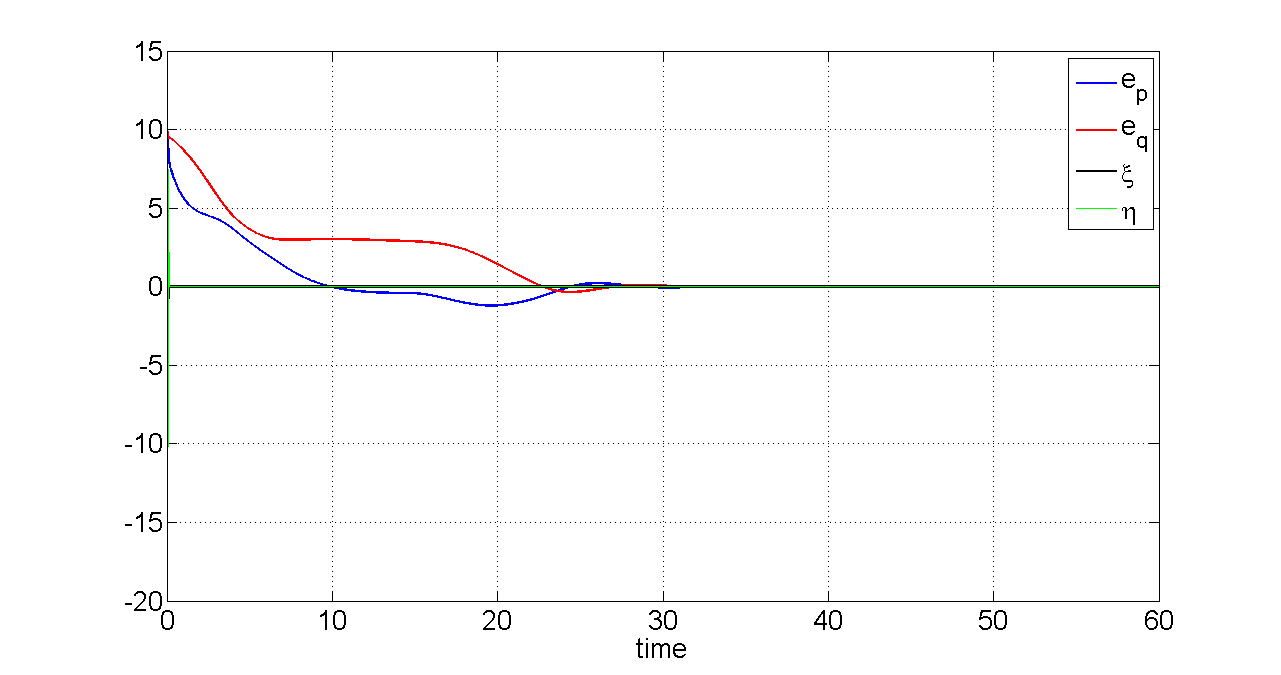
d​κm​a​x\displaystyle d\kappa_{max} has been chosen much smaller than 1\displaystyle 1 in order to emphasize upon significant initial conditions (in particular, ξ⁡(0)\displaystyle\xi(0) close to π\displaystyle\pi) so that the resultant illustrations highlight our claim. The initial conditions imposed upon the error are

ep​(0)=eq​(0)=10​m,ξ⁡(0)=9​π/10,e_{p}(0)=e_{q}(0)=10\ m,\ \xi(0)=9\pi/10,\

The parameters of the controller was taken as follow:

C1=0.1172,C2=0.5,k1=7500,k2=200,D=50.\displaystyle\displaystyle C_{1}=0.1172,\quad C_{2}=0.5,\quad k_{1}=7500,\quad k_{2}=200,\quad D=50.

Figure 2 shows the reference trajectory, the target point and vehicle in a 2D coordinate plane. It can be seen that the system converges to the reference trajectory asymptotically. Once the vehicle converges, the target point and the vehicle follow the trajectory very closely. The convergence can also be seen in the error graph shown in figure 3, where the initial conditions are also visible.

Figures 4 and 5 show the control signals u\displaystyle u and ρ\displaystyle\rho respectively. It is clear from these figures that the controller does not attain extremely large values, and is bounded. This is an essential property in real systems, which does not result in impossible control signals when the initial error is very large.

VI Conclusion

In this paper, we have addressed the problem of path following using a target point rigidly attached to a car type vehicle, by controlling only the orientation of the vehicle by its angular acceleration. The main idea was to determine a control law using saturation which ensures global stabilization in two steps. The proposed Lyapunov function forces the errors to enter a neighborhood of the origin in finite time. The Lyapunov analysis also shows that by a bootstrap procedure, this neighborhood contracts asymptotically to zero. Simulation results illustrate the GAS performance of the controller.

Refer to caption
Fig. 2: Reference trajectory, of the vehicle and its target point
Refer to caption
Fig. 3: Errors ep\displaystyle e_{p}, eq\displaystyle e_{q}, ξ\displaystyle\xi and η\displaystyle\eta
Refer to caption
Fig. 4: Control u\displaystyle u
Refer to caption
Fig. 5: Control ρ\displaystyle\rho

VII Proof of technical lemmas

VII-A Proof of Lemma III.4

One has

G⁡(s)=(s​I2−A)−1,\displaystyle\displaystyle\begin{array}[]{rcl}\begin{gathered}G\left(s\right)={\left({s{I_{2}}-A}\right)^{-1}},\hfill\\ \end{gathered}\end{array}

and the L2\displaystyle L_{2}-gain is defined by

ΥL=supω∈Rσ¯​(G⁡(j​ω)).\displaystyle\displaystyle\begin{array}[]{rcl}\begin{gathered}{{\rm{\Upsilon}}_{\rm{L}}}=\mathop{\sup}\nolimits_{\omega\in{R}}\bar{\sigma}(G(j\omega)).\hfill\\ \end{gathered}\end{array}

where σ¯\displaystyle\bar{\sigma} is the largest singular value of G⁡(j​ω)\displaystyle G(j\omega). Since

S⁡(ω):=G⁡(j​ω)​G∗​(j​ω)=ω2​I2+j​ω​(A−AT)+AT​A,S(\omega):=G(j\omega)G^{*}(j\omega)={{\omega^{2}}{I_{2}}+j\omega\left({A-{A^{T}}}\right)+{A^{T}}A},

one has that ΥL2\displaystyle{{\rm{\Upsilon}}_{\rm{L}}}^{2} is the inverse of the smallest eigenvalue of S⁡(ω)\displaystyle S(\omega).

We start the calculation of the matrix S⁡(ω)\displaystyle S(\omega) and get

S=[k12+ω2k1​k2+j​ω​(1+k1)k1​k2−j​ω​(1+k1)1+k22+ω2].\displaystyle\displaystyle\begin{array}[]{rcl}\begin{gathered}S=\left[{\begin{array}[]{*{20}{c}}{k_{1}^{2}+{\omega^{2}}}&{{k_{1}}{k_{2}}+j\omega\left({1+{k_{1}}}\right)}\\ {{k_{1}}{k_{2}}-j\omega\left({1+{k_{1}}}\right)}&{1+k_{2}^{2}+{\omega^{2}}}\\ \end{array}}\right].\end{gathered}\end{array}

The minimum eigenvalue is equal to

λm​i​n​(ω)=1+k12+k22+2​ω2−(1+k12+k22+2​ω2)2−4​(ω2​k22+(ω2−k1)2)2.\displaystyle\displaystyle\begin{array}[]{rcl}\begin{gathered}\lambda_{min}(\omega)=\frac{{1+k_{1}^{2}+k_{2}^{2}+2{\omega^{2}}-\sqrt{{{\left({1+k_{1}^{2}+k_{2}^{2}+2{\omega^{2}}}\right)}^{2}}-4\left({{\omega^{2}}k_{2}^{2}+{{\left({{\omega^{2}}-{k_{1}}}\right)}^{2}}}\right)}}}{2}.\end{gathered}\end{array}

The minimum of λm​i​n\displaystyle\lambda_{min} with respect to ω\displaystyle\omega is equal to

λm​i​n=1+k12+k222−(1−k12)2+k22​(k22+2+2​k12)4.\displaystyle\displaystyle\begin{array}[]{rcl}\begin{gathered}\lambda_{min}=\frac{{1+k_{1}^{2}+k_{2}^{2}}}{2}-\sqrt{\frac{{{(1-k_{1}^{2})}^{2}+k_{2}^{2}(k_{2}^{2}+2+2k_{1}^{2})}}{4}}.\end{gathered}\end{array}

We deduce that

ΥL2=12+1+k222​k12+12​1+(2​k2k1)2+(2​(1+k22)k12)2>1.\Upsilon_{L}^{2}=\frac{1}{2}+\frac{1+k_{2}^{2}}{2k_{1}^{2}}+\frac{1}{2}\sqrt{1+(\frac{2k_{2}}{k_{1}})^{2}+\Big(\frac{2(1+k_{2}^{2})}{k_{1}^{2}}\Big)^{2}}>1. (181)

If we tune k1=316​k22\displaystyle{k_{1}}=\frac{3}{{16}}k_{2}^{2} and k2≥20\displaystyle k_{2}\geq 20, then 0.93<λm​i​n<1\displaystyle 0.93<\lambda_{min}<1, and 1<ΥL<1.2\displaystyle 1<\Upsilon_{L}<1.2.

VII-B Proof of Lemma III.5

In that case, and by using the Taylor expansion of equation (181), we have the following asymptotic expansion of ΥL2\displaystyle\Upsilon_{L}^{2},

ΥL2=1+32​a2​k22+12​a2​k24+O⁡(1k26),\Upsilon_{L}^{2}=1+\frac{3}{2a^{2}k_{2}^{2}}+\frac{1}{2a^{2}k_{2}^{4}}+O(\frac{1}{k_{2}^{6}}), (182)

Then, the Riccati equation proposed in (III) takes the following form

(PkΥL+ΥL​A)T​(PkΥL+ΥL​A)=S, where ​S=−I+ΥL2​AT​A.\big(\frac{P_{k}}{\Upsilon_{L}}+\Upsilon_{L}A)^{T}\big(\frac{P_{k}}{\Upsilon_{L}}+\Upsilon_{L}A)=S,\hbox{ where }S=-I+\Upsilon_{L}^{2}A^{T}A. (183)

It can easily be checked that S\displaystyle S is definite positive since det(S)>0\displaystyle\det(S)>0:

S=[−1+ΥL2​a2​k24ΥL2​a​k23ΥL2​a​k23−1+ΥL2​(1+k22)],S=\left[{\begin{array}[]{*{20}{c}}{-1+\Upsilon_{L}^{2}{a^{2}}k_{2}^{4}}&{\Upsilon_{L}^{2}ak_{2}^{3}}\\ {\Upsilon_{L}^{2}ak_{2}^{3}}&{-1+\Upsilon_{L}^{2}\left({1+k_{2}^{2}}\right)}\\ \end{array}}\right],

and we get:

det(S)=ΥL2​k22​(a2​k22​(ΥL2−1)−1)−(ΥL2−1),\det(S)=\Upsilon_{L}^{2}k_{2}^{2}(a^{2}k_{2}^{2}(\Upsilon_{L}^{2}-1)-1)-(\Upsilon_{L}^{2}-1),

and we deduce from (181) the following Taylor expansion for det(S)\displaystyle\det(S),

det(S)=12​ΥL2​k22​(1+1k22+O⁡(1k24)).\det\left(S\right)=\frac{1}{2}\Upsilon_{L}^{2}k_{2}^{2}\big(1+\frac{1}{k_{2}^{2}}+O\left(\frac{1}{k_{2}^{4}}\right)\big).

Then, the Riccati equation (183), takes the form:

XT​X=S,{X^{T}}X=S,

where X=PkΥL+ΥL​A\displaystyle X=\frac{P_{k}}{\Upsilon_{L}}+\Upsilon_{L}A, and the solution is:

X=PkΥL+ΥL​A=Rϕ​S,X=\frac{P_{k}}{\Upsilon_{L}}+\Upsilon_{L}A=R_{\phi}\sqrt{S}, (184)

where Rϕ\displaystyle R_{\phi} is a rotation of angle ϕ\displaystyle\phi and S\displaystyle\sqrt{S} is the unique symmetric positive definite matrix whose square is equal to S\displaystyle S. We first estimate S\displaystyle\sqrt{S} and then ϕ\displaystyle\phi.

We clearly have

S=b​bT+γ​e2​e2T,S=bb^{T}+\gamma e_{2}e_{2}^{T},

where b=(αβ)\displaystyle b=\begin{pmatrix}\alpha\\ \beta\end{pmatrix}, e2=(01)\displaystyle e_{2}=\begin{pmatrix}0\\ 1\end{pmatrix} and

α=(ΥL​a​k22)2−1,β=ΥL2​a​k23α,γ=det(S)α2.\alpha=\sqrt{(\Upsilon_{L}ak_{2}^{2})^{2}-1},\quad\beta=\frac{\Upsilon_{L}^{2}ak_{2}^{3}}{\alpha},\quad\gamma=\frac{\det(S)}{\alpha^{2}}.

The asymptotic expansions of the above quantities are

(αβ)=ΥL​k2​(a​k2​(1−12​ΥL2​a2​k24+O⁡(1k28))1+12​ΥL2​a2​k24+O⁡(1k28)),γ=12​a2​k22​(1+1k22+O⁡(1k24)).\begin{pmatrix}\alpha\\ \beta\end{pmatrix}=\Upsilon_{L}k_{2}\begin{pmatrix}ak_{2}\big(1-\frac{1}{2\Upsilon_{L}^{2}a^{2}k_{2}^{4}}+O(\frac{1}{k_{2}^{8}})\big)\\ 1+\frac{1}{2\Upsilon_{L}^{2}a^{2}k_{2}^{4}}+O(\frac{1}{k_{2}^{8}})\end{pmatrix},\quad\gamma=\frac{1}{2a^{2}k_{2}^{2}}(1+\frac{1}{k_{2}^{2}}+O(\frac{1}{k_{2}^{4}})).

We also need the asymptotic expansions of the eigenvalues of S\displaystyle S. Since

S=[α2α​βα​ββ2+γ],S=\left[{\begin{array}[]{*{20}{c}}{{\alpha^{2}}}&{\alpha\beta}\\ {\alpha\beta}&{{\beta^{2}}+\gamma}\\ \end{array}}\right],

then,

λ1,2=α2+β2+γ±(α2+β2+γ)2−4​α2​γ2{\lambda_{1,2}}=\frac{\alpha^{2}+\beta^{2}+\gamma\pm\sqrt{\left(\alpha^{2}+\beta^{2}+\gamma\right)^{2}-4\alpha^{2}\gamma}}{2}

We immediately deduce the following asymptotic expansions for the eigenvalues of S\displaystyle S,

λ1=α2+β2+O⁡(1k24),λ2=γ⁡(1+O⁡(1k22)).\lambda_{1}=\alpha^{2}+\beta^{2}+O(\frac{1}{k_{2}^{4}}),\quad\lambda_{2}=\gamma(1+O(\frac{1}{k_{2}^{2}})). (185)

We use b¯\displaystyle\bar{b} to denote the unit vector b/‖b‖\displaystyle b/\|b\| and define the angle ϕb\displaystyle\phi_{b} so that Rϕb​e1=b¯\displaystyle R_{\phi_{b}}e_{1}=\bar{b}, where e1=(10)\displaystyle e_{1}=\begin{pmatrix}1\\ 0\end{pmatrix}.

We have

‖b‖=ΥL​a​k22​(1+12​a2​k22+O⁡(1k24)),b¯=(1−12​a2​k22+O⁡(1k24)1a​k2​(1+12​a2​k22+O​(1k24))),\|b\|=\Upsilon_{L}ak_{2}^{2}\big(1+\frac{1}{2a^{2}k_{2}^{2}}+O(\frac{1}{k_{2}^{4}})\big),\qquad\bar{b}=\begin{pmatrix}1-\frac{1}{2a^{2}k_{2}^{2}}+O(\frac{1}{k_{2}^{4}})\\ \frac{1}{ak_{2}}\big(1+\frac{1}{2a^{2}k_{2}^{2}}+O(\frac{1}{k_{2}^{4}})\big)\end{pmatrix},

and

Rϕb=l2​I​d2+l1​A0,R_{\phi_{b}}=l_{2}Id_{2}+l_{1}A_{0},

where A0=(0−110)\displaystyle A_{0}=\begin{pmatrix}0&-1\\ 1&0\end{pmatrix} and

l1=1a​k2​(1−32​a2​k22+O⁡(1k24)),l2=(1−12​a2​k22+O⁡(1k24)).l_{1}=\frac{1}{ak_{2}}\big(1-\frac{3}{2a^{2}k_{2}^{2}}+O(\frac{1}{k_{2}^{4}})\big),\qquad l_{2}=(1-\frac{1}{2a^{2}k_{2}^{2}}+O(\frac{1}{k_{2}^{4}})).

We then get that R−ϕb​e2=l2​e2−l1​e1\displaystyle R_{-\phi_{b}}e_{2}=l_{2}e_{2}-l_{1}e_{1}. We can therefore write

R−ϕb​S​Rϕb=‖b‖2​e1​e1T+γ​R−ϕb​e2​e2T​Rϕb,R_{-\phi_{b}}SR_{\phi_{b}}=\|b\|^{2}e_{1}e_{1}^{T}+\gamma R_{-\phi_{b}}e_{2}e_{2}^{T}R_{\phi_{b}},

and deduce that

R−ϕb​S​Rϕb=(‖b‖2+γ​l12)​e1​e1T+γ​l22​e2​e2T−γ​l1​l2​(e1​e2T+e2​e1T).R_{-\phi_{b}}SR_{\phi_{b}}=(\|b\|^{2}+\gamma l_{1}^{2})e_{1}e_{1}^{T}+\gamma l_{2}^{2}e_{2}e_{2}^{T}-\gamma l_{1}l_{2}(e_{1}e_{2}^{T}+e_{2}e_{1}^{T}). (186)

Finally, we seek a formula of the type

R−ϕb​S​Rϕb=s1​e1​e1T+s2​e2​e2T−s3​(e1​e2T+e2​e1T),R_{-\phi_{b}}\sqrt{S}R_{\phi_{b}}=s_{1}e_{1}e_{1}^{T}+s_{2}e_{2}e_{2}^{T}-s_{3}(e_{1}e_{2}^{T}+e_{2}e_{1}^{T}), (187)

where the sI\displaystyle s_{I}’s are positive. A simple identification leads to the equations

s12+s32=‖b‖2+γ​l12,s22+s32=γ​l22,s3=γ​l1​l2T​r​(S).s_{1}^{2}+s_{3}^{2}=\|b\|^{2}+\gamma l_{1}^{2},\qquad s_{2}^{2}+s_{3}^{2}=\gamma l_{2}^{2},\qquad s_{3}=\frac{\gamma l_{1}l_{2}}{Tr(\sqrt{S})}.

We deduce at once from the asymptotic expansions of the eigenvalues of S\displaystyle S obtained in (185) that

s1=‖b‖​(1+O⁡(1k28)),s2=γ​(1+O⁡(1k22)),s3=O⁡(1k25).s_{1}=\|b\|(1+O(\frac{1}{k_{2}^{8}})),\qquad s_{2}=\sqrt{\gamma}(1+O(\frac{1}{k_{2}^{2}})),\qquad s_{3}=O(\frac{1}{k_{2}^{5}}). (188)

From the expression ΥL​(A−AT)=Rϕ​S−S​R−ϕ\displaystyle\Upsilon_{L}(A-A^{T})=R_{\phi}\sqrt{S}-\sqrt{S}R_{-\phi}, we obtain

ΥL​(1+a​k22)​[01−10]=−T​r​(S)​sin⁡(ϕ)​[01−10],{\Upsilon_{L}}\left({1+ak_{2}^{2}}\right)\left[{\begin{array}[]{*{20}{c}}0&1\\ {-1}&0\\ \end{array}}\right]=-Tr\left({\sqrt{S}}\right)\sin\left(\phi\right)\left[{\begin{array}[]{*{20}{c}}0&1\\ {-1}&0\\ \end{array}}\right],

and we deduce that ΥL​(1+a​k22)=−T​r​(S)​sin⁡(ϕ)\displaystyle\Upsilon_{L}(1+ak_{2}^{2})=-Tr(\sqrt{S})\sin(\phi), i.e.,

sin⁡(ϕ)=−(1−C022​k22+O⁡(1k23)),\sin(\phi)=-\big(1-\frac{C_{0}^{2}}{2k_{2}^{2}}+O(\frac{1}{k_{2}^{3}})\big),

where C0=1−2​aa\displaystyle C_{0}=\frac{\sqrt{1-2a}}{a}. It implies that

Rϕ=C0k2​(1+O⁡(1k2))​I​d2−(1−C022​k22+O⁡(1k23))​A0.R_{\phi}=\frac{C_{0}}{k_{2}}\big(1+O(\frac{1}{k_{2}})\big)Id_{2}-\big(1-\frac{C_{0}^{2}}{2k_{2}^{2}}+O(\frac{1}{k_{2}^{3}})\big)A_{0}.

We now collect the result of the equation (184) and (188) to get,

PkΥL=−ΥLA+RϕRϕb[s1e1e1T+s2e2e2T+O(1k25))]R−ϕb.\frac{P_{k}}{\Upsilon_{L}}=-\Upsilon_{L}A+R_{\phi}R_{\phi_{b}}\Big[s_{1}e_{1}e_{1}^{T}+s_{2}e_{2}e_{2}^{T}+O(\frac{1}{k_{2}^{5}}))\Big]R_{-\phi_{b}}.

After a long but straightforward computation, we arrive at (122).

VII-C Proof of Proposition III.6

Proof.

The proof is developed using Young inequality, |η​ξ|≤ϵ​η22+ξ22​ϵ\displaystyle|\eta\xi|\leq\frac{\epsilon\eta^{2}}{2}+\frac{\xi^{2}}{2\epsilon}, where ϵ\displaystyle\epsilon is an arbitrary positive constant.

First of all, according to Lemma III.5, for large k2\displaystyle k_{2}, the quadratic form Vk​(ξ,η)\displaystyle V_{k}(\xi,\eta) satisfies the following inequality

Vk​(ξ,η)≥F1​k2​ξ2+2​F2​ξ​η+F3​η2k2−Ck2​(ξ2+η2k22),V_{k}(\xi,\eta)\geq F_{1}k_{2}\xi^{2}+2F_{2}\xi\eta+F_{3}\frac{\eta^{2}}{k_{2}}-\frac{C}{k_{2}}(\xi^{2}+\frac{\eta^{2}}{k_{2}^{2}}),

for some positive universal constant C>0\displaystyle C>0. Then, by setting X:=k2​F1​η\displaystyle X:=\sqrt{k_{2}F_{1}}\eta and Y:=ηk2​F3\displaystyle Y:=\frac{\eta}{\sqrt{k_{2}F_{3}}}, we obtain

Vk​(ξ,η)≥(1−Ck22)​X2+2​F2F1​F3​X​Y+(1−Ck22)​Y2.V_{k}(\xi,\eta)\geq(1-\frac{C}{k_{2}^{2}})X^{2}+2\frac{F_{2}}{\sqrt{F_{1}F_{3}}}XY+(1-\frac{C}{k_{2}^{2}})Y^{2}.

Since F22F1​F3<1\displaystyle\frac{F_{2}^{2}}{F_{1}F_{3}}<1, the above inequality ensures, for k2\displaystyle k_{2} large enough, the existence of l>0\displaystyle l>0 only dependent of a\displaystyle a such that

Vk​(ξ,η)≥l⁡(k2​ξ2+η2k2).V_{k}(\xi,\eta)\geq l\left(k_{2}\xi^{2}+\frac{\eta^{2}}{k_{2}}\right).

The previous inequality with M=β​k2\displaystyle M=\beta k_{2} and k1=a​k22\displaystyle k_{1}=ak_{2}^{2} computed in (III) implies

V⁡(y1,y2,ξ,η)\displaystyle\displaystyle V(y_{1},y_{2},\xi,\eta) ≥\displaystyle\displaystyle\geq l​β​k22​ξ2+l​β​η2+a​k222​(y12+y22)−|η​y2|−|k2​y2​ξ|.\displaystyle\displaystyle l\beta k_{2}^{2}\xi^{2}+l\beta\eta^{2}+\frac{ak_{2}^{2}}{2}\left(y_{1}^{2}+y_{2}^{2}\right)-\left|\eta y_{2}\right|-\left|k_{2}y_{2}\xi\right|.

By using Young’s inequality, we get

|η​y2|\displaystyle\displaystyle\left|\eta y_{2}\right| ≤\displaystyle\displaystyle\leq l​β​η22+1l​β​y222,\displaystyle\displaystyle l\beta\frac{\eta^{2}}{2}+\frac{1}{l\beta}\frac{y_{2}^{2}}{2},
|k2​y2​ξ|\displaystyle\displaystyle\left|k_{2}y_{2}\xi\right| ≤\displaystyle\displaystyle\leq l​β​k22​ξ22+1l​β​y222.\displaystyle\displaystyle l\beta\frac{k_{2}^{2}\xi^{2}}{2}+\frac{1}{l\beta}\frac{y_{2}^{2}}{2}.

Which implies,

V≥(a​k222+1l​β)​y22+l​β​k222​ξ2+l​β2​η2+a​k222​y12.\displaystyle\displaystyle V\geq\left(\frac{ak_{2}^{2}}{2}+\frac{1}{l\beta}\right)y_{2}^{2}+\frac{l\beta k_{2}^{2}}{2}\xi^{2}+\frac{l\beta}{2}\eta^{2}+\frac{ak_{2}^{2}}{2}y_{1}^{2}.

then for large enough k2\displaystyle k_{2}, V\displaystyle V is a positive quadratic form in (ξ,η,y1,y2)\displaystyle(\xi,\eta,y_{1},y_{2}). ∎

VII-D Proof of Lemma III.7

The solution of the equation (III) is

Z⁡(t)=∫0teA⁡(t−s)​U​(s)​𝑑s+eA​t​Z0,\displaystyle\displaystyle\begin{array}[]{rcl}\begin{gathered}Z\left(t\right)=\int_{0}^{t}{e^{A\left({t-s}\right)}}U\left(s\right)ds+{e^{At{Z_{0}}}},\end{gathered}\end{array}

where Z0\displaystyle Z_{0} is the initial value of Z\displaystyle Z for t=0\displaystyle t=0. We start by diagonalization of the matrix A\displaystyle A, whose eigenvalues are equal to

λ+=−k22+12​k22−4​k1,λ−=−k22−12​k22−4​k1,\displaystyle\displaystyle\begin{array}[]{rcl}\begin{gathered}{\lambda_{+}}=-\frac{{{k_{2}}}}{2}+\frac{1}{2}\sqrt{k_{2}^{2}-4{k_{1}}},\\ {\lambda_{-}}=-\frac{{{k_{2}}}}{2}-\frac{1}{2}\sqrt{k_{2}^{2}-4{k_{1}}},\\ \end{gathered}\end{array}

with corresponding eigenvectors V+=(1λ+)\displaystyle{V_{+}}=\left({\begin{array}[]{*{20}{c}}1\\ {{\lambda_{+}}}\\ \end{array}}\right) and V−=(1λ−)\displaystyle{V_{-}}=\left({\begin{array}[]{*{20}{c}}1\\ {{\lambda_{-}}}\\ \end{array}}\right). From here, we obtain A=P​D​P−1\displaystyle A=PD{P^{-1}}, where

D=(λ+00λ−),P=(V+V−)=(1λ+1λ−);\displaystyle\displaystyle\begin{array}[]{rcl}\begin{gathered}{\kern 1.0pt}D=\left({\begin{array}[]{*{20}{c}}{{\lambda_{+}}}&0\\ 0&{{\lambda_{-}}}\\ \end{array}}\right);{\kern 1.0pt}P=\left({\begin{array}[]{*{20}{c}}{{V_{+}}}&{{V_{-}}}\\ \end{array}}\right)=\left({\begin{array}[]{*{20}{c}}{\begin{array}[]{*{20}{c}}1\\ {{\lambda_{+}}}\\ \end{array}}&{\begin{array}[]{*{20}{c}}1\\ {{\lambda_{-}}}\\ \end{array}}\\ \end{array}}\right);\end{gathered}\end{array}

We get

eA⁡(t−s)​U​(s)=1λ−−λ+​((λ−​v1−v2)​eλ+​(t−s)+(λ+​v1+v2)​eλ−​(t−s)λ+​(λ−​v1−v2)​eλ+​(t−s)+λ−​(λ+​v1+v2)​eλ−​(t−s))\displaystyle\displaystyle\begin{array}[]{l}{e^{A\left({t-s}\right)}}U\left(s\right)=\frac{1}{{{\lambda_{-}}-{\lambda_{+}}}}\left({\begin{array}[]{*{20}{c}}{\left({{\lambda_{-}}{v_{1}}-{v_{2}}}\right){e^{{\lambda_{+}}\left({t-s}\right)}}+\left({{\lambda_{+}}{v_{1}}+{v_{2}}}\right){e^{{\lambda_{-}}\left({t-s}\right)}}}\\ {{\lambda_{+}}\left({{\lambda_{-}}{v_{1}}-{v_{2}}}\right){e^{{\lambda_{+}}\left({t-s}\right)}}+{\lambda_{-}}\left({{\lambda_{+}}{v_{1}}+{v_{2}}}\right){e^{{\lambda_{-}}\left({t-s}\right)}}}\\ \end{array}}\right)\\ \end{array}

The control variables ν1\displaystyle\nu_{1} and ν2\displaystyle\nu_{2} are bounded respectively by κm​a​x​C1\displaystyle\kappa_{max}C_{1} and C2\displaystyle C_{2} and we obtain that the components of the vector ∫0teA⁡(t−s)​U​(s)​𝑑s\displaystyle\int_{0}^{t}{e^{A\left({t-s}\right)}}U\left(s\right)ds are bounded componentwise by

(1|λ+|​(κm​a​x​C1+C2|λ−|)κm​a​x​C1+C2|λ+|+C2|λ−|.).\displaystyle\displaystyle\begin{array}[]{rcl}\begin{gathered}\left(\begin{array}[]{c}\begin{array}[]{*{20}{c}}{\frac{1}{{\left|{\begin{array}[]{*{20}{c}}{{\lambda_{+}}}\\ \end{array}}\right|}}\left({\kappa_{max}{C_{1}}+\frac{{{C_{2}}}}{{\left|{{\lambda_{-}}}\right|}}}\right)}\\ \end{array}\\ \kappa_{max}{C_{1}}+\frac{{{C_{2}}}}{{\left|{{\lambda_{+}}}\right|}}+\frac{{{C_{2}}}}{{\left|{{\lambda_{-}}}\right|.}}\\ \end{array}\right).\end{gathered}\end{array}

By taking k1=316​k22\displaystyle k_{1}=\frac{3}{16}k_{2}^{2}, we get λ+=−k24\displaystyle{\lambda_{+}}=-\frac{{{k_{2}}}}{4} and λ−=−3​k24\displaystyle{\lambda_{-}}=-\frac{{3{k_{2}}}}{4}. We can bound the components of the vector defined in (II) by

(4k2​(κm​a​x​C1+43​k2​C2)κm​a​x​C1+163​k2​C2).\displaystyle\displaystyle\begin{array}[]{rcl}\begin{gathered}\left(\begin{array}[]{c}\begin{array}[]{*{20}{c}}{\frac{4}{k_{2}}\left({\kappa_{max}{C_{1}}+\frac{4}{{3{k_{2}}}}{C_{2}}}\right)}\\ \end{array}\\ \kappa_{max}{C_{1}}+\frac{{16}}{{3{k_{2}}}}{C_{2}}\\ \end{array}\right).\end{gathered}\end{array}

Equation (III.7) can be deduced directly from Equations (VII-D) and (VII-D). Moreover, since A\displaystyle A is Hurwitz, we arrive to (III.7).

VII-E Proof of Lemma III.10

The terms |η​ξ|\displaystyle|\eta\xi| and k2​ξ2\displaystyle{k_{2}}\xi^{2} are clearly dominated by M4​(ξ2+η2)\displaystyle\frac{M}{4}({\xi^{2}+\eta^{2}}).

In (III.9), one has M​(ΥL​κr​C1​σ​(y1))2≤C​M​(C1​σ​(y1))2\displaystyle M\big(\Upsilon_{L}\kappa_{r}C_{1}\sigma(y_{1})\big)^{2}\leq CM\big(C_{1}\sigma(y_{1})\big)^{2}, which is dominated by k1​C14​y1​σ​(y1)\displaystyle\frac{k_{1}C_{1}}{4}y_{1}\sigma(y_{1}) if C​β​C1≤a​k24\displaystyle C\beta C_{1}\leq\frac{ak_{2}}{4}. The latter clearly holds true for k2\displaystyle k_{2} large enough.

We have M​(ΥL​C2​σ​(y2))2≤C​M​(C2​σ​(y2))2\displaystyle M\big(\Upsilon_{L}C_{2}\sigma(y_{2})\big)^{2}\leq CM\big(C_{2}\sigma(y_{2})\big)^{2}, which is dominated by C2​y2​σ​(y2)/4\displaystyle C_{2}y_{2}\sigma(y_{2})/4 if A​M​C22≤C2/4\displaystyle AMC_{2}^{2}\leq C_{2}/4. The latter is true according to the choice of C2\displaystyle C_{2} in (72).

We now turn to the control of the term k2​C1​|y2​κr​σ​(y1)|\displaystyle k_{2}C_{1}|y_{2}\kappa_{r}\sigma(y_{1})| by k1​C14​y1​σ​(y1)+C24​y2​σ​(y2)\displaystyle\frac{k_{1}C_{1}}{4}y_{1}\sigma(y_{1})+\frac{C_{2}}{4}y_{2}\sigma(y_{2}). If |y2|≥1\displaystyle|y_{2}|\geq 1, the second term is in control if C24≥C​k2​C1\displaystyle\frac{C_{2}}{4}\geq Ck_{2}C_{1} which holds true. Assume now that |y2|≤1\displaystyle|y_{2}|\leq 1. In the case where |y1|≥1\displaystyle|y_{1}|\geq 1, the first term is in control if k1​C14≥C​k2​C1\displaystyle\frac{k_{1}C_{1}}{4}\geq Ck_{2}C_{1} which obviously holds true. It remains the case where |y1|≤1\displaystyle|y_{1}|\leq 1. It is immediate to check that the quadratic form k1​C14​y12+C24​y22−C​k2​C1​y1​y2\displaystyle\frac{k_{1}C_{1}}{4}y_{1}^{2}+\frac{C_{2}}{4}y_{2}^{2}-Ck_{2}C_{1}y_{1}y_{2} is definite positive.

We next consider the term k1​|y2|​|ξ|3\displaystyle k_{1}|y_{2}||\xi|^{3}. To control it, we first bound |ξ|2\displaystyle|\xi|^{2} by Ck26\displaystyle\frac{C}{k_{2}^{6}} for t\displaystyle t large enough. In case |y2|≥1\displaystyle|y_{2}|\geq 1, then the term is immediately dominated by C24​|y2|\displaystyle\frac{C_{2}}{4}|y_{2}|. Otherwise, one has, for k2\displaystyle k_{2} large enough,

k1​|y2|​|ξ|3≤C​|y2|k2​|ξ|k24≤C⁡(y22k22+ξ2k24),k_{1}|y_{2}||\xi|^{3}\leq C\frac{|y_{2}|}{k_{2}}\frac{|\xi|}{k_{2}^{4}}\leq C(\frac{y_{2}^{2}}{k_{2}^{2}}+\frac{\xi^{2}}{k_{2}^{4}}),

the last two terms being controlled by C24​|y2|2+M4​ξ2\displaystyle\frac{C_{2}}{4}|y_{2}|^{2}+\frac{M}{4}\xi^{2}.

Using again the estimate |ξ|\displaystyle|\xi| by Ck23\displaystyle\frac{C}{k_{2}^{3}} for t\displaystyle t large enough, the control of k1​|y1|​|ξ|2\displaystyle k_{1}|y_{1}||\xi|^{2} reduces to that of k2​|y1​ξ|\displaystyle k_{2}|y_{1}\xi|. It therefore remain to control the latter. This is where we need the hypothesis that y∉Yk2\displaystyle y\notin Y_{k_{2}}. Assume first that one wants to get the inequality

k2​|y1​ξ|≤k1​C14​y1​σ​(y1).k_{2}|y_{1}\xi|\leq\frac{k_{1}C_{1}}{4}y_{1}\sigma(y_{1}). (225)

This holds true if |y1|≥Ck22\displaystyle|y_{1}|\geq\frac{C}{k_{2}^{2}}. On the other hand, if one wants to get the inequality

k2​|y1​ξ|≤C24​y2​σ​(y2),k_{2}|y_{1}\xi|\leq\frac{C_{2}}{4}y_{2}\sigma(y_{2}), (226)

it holds if |y2|≥Ck23/2\displaystyle|y_{2}|\geq\frac{C}{k_{2}^{3/2}}. In any case, outside Yk2\displaystyle Y_{k_{2}}, one of the two inequalities (225) or (226) must hold true and LemmaIII.10 is established.

Finally, with the choice of M=β​k2\displaystyle M=\beta k_{2} together with (122), it is immediate to verfy that V\displaystyle V is positive definite. Moreover, we get

a1​k2​ξ2+a2k2​η2+a3​k22​(y12+y22)≤V≤d1​k2​ξ2+d2k2​η2+d3​k22​(y12+y22),a_{1}k_{2}\xi^{2}+\frac{a_{2}}{k_{2}}\eta^{2}+a_{3}k_{2}^{2}(y_{1}^{2}+y_{2}^{2})\leq V\leq d_{1}k_{2}\xi^{2}+\frac{d_{2}}{k_{2}}\eta^{2}+d_{3}k_{2}^{2}(y_{1}^{2}+y_{2}^{2}), (227)

for some positive constants ai\displaystyle a_{i}, di\displaystyle d_{i}, 1≤i≤3\displaystyle 1\leq i\leq 3.

References

  • [1] C. Samson and K. AitAbderrahim. Feedback control of a nonholonomic wheeled cart in Cartesian space. IEEE international conference on robotics and automation, Sacramento, California, USA, 2:1136 – 1141, 1991.
  • [2] L. Consolini, A. Piazzi, and M. Tosques. Motion planning for steering car-like vehicles. Proc. European Control Conference, Porto, Portugal, pages 1834–1839, 2001.
  • [3] Z. P. Jiang, E. Lefeber, and H. Nijmeijer. Saturated stabilization and tracking of a nonholonomic mobile robot. Systems & Control Letters, 42:327–332, 2001.
  • [4] C. Samson. Control of chained systems application to path following and time-varying point-stabilization of mobile robots. IEEE Transactions on Automatic Control, 40(1):64–76, 1995.
  • [5] M. Egerstedt, X. Hu, and A. Stotsky. Control of mobile platforms using a virtual vehicle approach. IEEE Transactions on Automatic Control, 46(11):1777–1782, 2001.
  • [6] C. Guarino Lo Bianco, A. Piazzi, and M. Romano. Smooth motion generation for unicycle mobile robots via dynamic path inversion. IEEE Transactions on Robotics, 20(5):884–891, 2004.
  • [7] M. Fliess, J. Levine, P. Martin, and P. Rouchon. A lie–backlund approach to equivalence and flatness of nonlinear systems. IEEE Transactions on Automatic Control, 44:922––937, 1999.
  • [8] P. Rouchon, M. Fliess, J. Levine, and P. Martin. Flatness and motion planning: the car with n trailers. Proceedings of the European Control Conference, ECC’93, Groninge, Netherlands, pages 1518––1522, 1993.
  • [9] Z. P. Jiang and H. Nijmeijer. Tracking control of mobile robots: A case study in backstepping. Automatica, 33:1393–1399, 1997.
  • [10] C. Low and D. Wang. Robust path following of car-like wmr in the presence of skidding effects. Proceedings of 2005 IEEE Intl. Conf. Mechatronics, Taipei, Taiwan, pages 864–869, 2005.
  • [11] K. D. Do, Z. P. Jiang, and J. Pan. A global output-feedback controller for simultaneous tracking and stabilization of unicycle-type mobile robots. IEEE Transactions on Robotics and Automation, 20(3):589––594, 2004.
  • [12] K. D. Do, Z. P. Jiang, and J. Pan. Simultaneous tracking and stabilization of mobile robots: an adaptive approach. IEEE Transactions on Automatic Control, 49(7):1147––1152, 2004.
  • [13] A. Pedro Aguiar and J. P. Hespanha. Trajectory-traking and path-following of underactuated autonomous vehicles with parametric modeling uncertainty. IEEE Transactions on Automatic Control, 52(8):1362–1378, 2007.
  • [14] Anthony Bloch and Sergey Drakunov. Stabilization and tracking in the nonholonomic integrator via sliding modes. Syst. Control Lett., 29(2):91–99, October 1996.
  • [15] Ti-Chung Lee, Kai-Tai Song, Ching-Hung Lee, and Ching-Cheng Teng. Tracking control of unicycle-modeled mobile robots using a saturation feedback controller. IEEE Transactions on Control Systems Technology, 8(2):305–318, 2001.
  • [16] A. Broggi, M. Bertozzi, A. Fascioli, C. Guarino Lo Bianco, and A. Piazzi. The argo autonomous vehicle’s vision and control systems. Int. J. Intelligent Control and Systems, 3:409–441, 1999.
  • [17] A. Piazzi, C. Guarino Lo Bianco, M. Bertozzi, A. Fascioli, and A. Broggi. Quintic g2-splines for the iterative steering of vision-based autonomous vehicles. IEEE Transactions on Intelligent Transportations Systems, 3:27––36, 2002.
  • [18] M. Bertozzi and A. Broggi. Gold: a parallel realtime stereo vision system for generic obstacle and lane detection. IEEE Transactions on Image Processing, 7:62––81, 1998.
  • [19] L. Consolini, A. Piazzi, and M. Tosques. Path following of car-like vehicles using dynamic inversion. Int. J. Control, 76(17):1724–1738, 2003.
  • [20] P. Morin and C. Samson. Trajectory tracking for non-holonomic vehicles: overview and case study. Proc. Fourth International Workshop on Robot Motion and Control, Puszczykowo, Poland, pages 139–153, 2004.
  • [21] W. Pasillas-Lepine. Hybrid modelling and limit cycle analysis for a class of anti-lock brake algorithms. In International Symposium on Advanced Vehicle Control, Arnhem, The Netherlands, 2004.
  • [22] Yacine Chitour, Wensheng Liu, and Eduardo Sontag. On the continuity and incremental-gain properties of certain saturated linear feedback loops. International Journal of Robust and Nonlinear Control, 5(5):413–440, 1995.
  • [23] W. Liu, Y. Chitour, and E. Sontag. On finite-gain stabilizability of linear systems subject to input saturation. SIAM Journal on Control and Optimization, 34(4):1190–1219, 1996.
  • [24] K. Yakoubi and Y. Chitour. Linear systems subject to input saturation and time delay: Finite-gain lp\displaystyle l^{p}-stabilization. SIAM Journal on Control and Optimization, 45(3):1084–1115, 2006.
  • [25] K. Yakoubi and Y. Chitour. Linear systems subject to input saturation and time delay: Global asymptotic stabilization. Automatic Control, IEEE Transactions on, 52(5):874 –879, 2007.
  • [26] Karim Yakoubi and Yacine Chitour. Stabilization and finite-gain stabilizability of delay linear systems subject to input saturation. In Applications of Time Delay Systems, volume 352 of Lecture Notes in Control and Information Sciences, pages 329–341. Springer Berlin Heidelberg, 2007.
  • [27] Karim Yakoubi and Yacine Chitour. On the stabilization of linear discrete-time delay systems subject to input saturation. In Advanced strategies in control systems with input and output constraints, volume 352 of Lecture Notes in Control and Information Sciences, page 421–455. Springer Berlin Heidelberg, 2007.
  • [28] S. Laghrouche, Y. Chitour, M. Harmouche, and F. S. Ahmed. Path Following for a Target Point Attached to a Unicycle Type Vehicle. Acta Applicanda Mathematicae (2012).
  • [29] L. Ljung and T. Soderstrom. Theory and Practice of Recursive Identification. The MIT Press, Cambridge, MA. USA., 1983.
  • [30] Hassan K. Khalil. Nonlinear Systems (3r​d\displaystyle 3^{rd} ed.). Prentice Hall, New Jersey, USA, 2002.
  • [31] Y. Chitour. On the lp\displaystyle l^{p}-stabilization of the double integrator subject to input saturation. ESAIM: Control, Optimisation and Calculus of Variations, 6:291–331, March 2001.
  • [32] A. Gruszka, M. Malisoff, and F. Mazenc. Tracking Control and Robustness Analysis for PVTOL Aircraft under Bounded Feedbacks. Internat. J. Robust Nonlinear Control (2011).
  • [33] M.T. Angulo, J.A. Moreno, and L. Fridman. An exact and uniformly convergent arbitrary order differentiator. In Decision and Control and European Control Conference (CDC-ECC), 2011 50th IEEE Conference on, pages 7629 –7634, dec. 2011.