Planck 2013 results. I. Overview of products and scientific results
Abstract
The European Space Agency’s Planck satellite, dedicated to studying the early Universe and its subsequent evolution, was launched 14 May 2009 and has been scanning the microwave and submillimetre sky continuously since 12 August 2009. In March 2013, ESA and the Planck Collaboration released the initial cosmology products based on the the first 15.5 months of Planck data, along with a set of scientific and technical papers and a web-based explanatory supplement. This paper gives an overview of the mission and its performance, the processing, analysis, and characteristics of the data, the scientific results, and the science data products and papers in the release. The science products include maps of the cosmic microwave background (CMB) and diffuse extragalactic foregrounds, a catalogue of compact Galactic and extragalactic sources, and a list of sources detected through the Sunyaev-Zeldovich effect. The likelihood code used to assess cosmological models against the Planck data and a lensing likelihood are described. Scientific results include robust support for the standard six-parameter CDM model of cosmology and improved measurements of its parameters, including a highly significant deviation from scale invariance of the primordial power spectrum. The Planck values for these parameters and others derived from them are significantly different from those previously determined. Several large-scale anomalies in the temperature distribution of the CMB, first detected by WMAP, are confirmed with higher confidence. Planck sets new limits on the number and mass of neutrinos, and has measured gravitational lensing of CMB anisotropies at greater than . Planck finds no evidence for non-Gaussianity in the CMB. Planck’s results agree well with results from the measurements of baryon acoustic oscillations. Planck finds a lower Hubble constant than found in some more local measures. Some tension is also present between the amplitude of matter fluctuations () derived from CMB data and that derived from Sunyaev-Zeldovich data. ThePlanck and WMAP power spectra are offset from each other by an average level of about 2% around the first acoustic peak. Analysis of Planck polarization data is not yet mature, therefore polarization results are not released, although the robust detection of -mode polarization around CMB hot and cold spots is shown graphically.
Key Words.
Cosmology: observations — Cosmic background radiation — Surveys — Space vehicles: instruments — Instrumentation: detectors1 Introduction
The Planck satellite11 1 Planck (http://www.esa.int/Planck) is a project of the European Space Agency (ESA) with instruments provided by two scientific consortia funded by ESA member states (in particular the lead countries, France and Italy) with contributions from NASA (USA), and telescope reflectors provided in a collaboration between ESA and a scientific consortium led and funded by Denmark. (Tauber et al. 2010a; Planck Collaboration I 2011) was launched on 14 May 2009 and observed the sky stably and continuously from 12 August 2009 to 23 October 2013. Planck’s scientific payload comprised an array of 74 detectors sensitive to frequencies between 25 and 1000 GHz, which scanned the sky with angular resolution between 33′ and 5′. The detectors of the Low Frequency Instrument (Bersanelli et al. 2010; Mennella et al. 2011, LFI;) are pseudo-correlation radiometers, covering bands centred at 30, 44, and 70 GHz. The detectors of the High Frequency Instrument (Lamarre et al. 2010; Planck HFI Core Team 2011a, HFI;) are bolometers, covering bands centred at 100, 143, 217, 353, 545, and GHz. Planck images the whole sky twice in one year, with a combination of sensitivity, angular resolution, and frequency coverage never before achieved. Planck, its payload, and its performance as predicted at the time of launch are described in 13 papers included in a special issue of Astronomy & Astrophysics (Volume 520).
The main objective of Planck, defined in 1995, is to measure the spatial anisotropies in the temperature of the cosmic microwave background (CMB), with an accuracy set by fundamental astrophysical limits, thereby extracting essentially all the cosmological information embedded in the temperature anisotropies of the CMB. Planck was also designed to measure to high accuracy the CMB polarization anisotropies, which encode not only a wealth of cosmological information, but also provide a unique probe of the early history of the Universe during the time when the first stars and galaxies formed. Finally, Planck produces a wealth of information on the properties of extragalactic sources and on the dust and gas in the Milky Way (see Fig. 1). The scientific objectives of Planck are described in detail in Planck Collaboration (2005). With the results presented here and in a series of accompanying papers (see Fig. 2), Planck has already achieved many of its planned science goals.

This paper presents an overview of the Planck mission, and the main data products and scientific results of Planck’s second release22 2 In January of 2011, ESA and the Planck Collaboration released to the public a first set of scientific data, the Early Release Compact Source Catalogue (ERCSC), a list of unresolved and compact sources extracted from the first complete all-sky survey carried out by Planck (Planck Collaboration VII 2011). At the same time, initial scientific results related to astrophysical foregrounds were published in a special issue of Astronomy and Astrophysics (Vol 520, 2011). Since then, 12 “Intermediate” papers have been submitted for publication to A&A containing further astrophysical investigations by the Collaboration., based on data acquired in the period 12 August 2009 to 28 November 2010.
1.1 Overview of 2013 science results
Cosmology—A major goal of Planck is to measure the key cosmological parameters describing our Universe. Planck’s combination of sensitivity, angular resolution, and frequency coverage enables it to measure anisotropies on intermediate and small angular scales over the whole sky much more accurately than previous experiments. This leads to improved constraints on individual parameters, the breaking of degeneracies between combinations of other parameters, and less reliance on supplementary astrophysical data than previous CMB experiments. Cosmological parameters are presented and discussed in Sect. 9 and in Planck Collaboration XVI (2014).
The Universe observed by Planck is well-fit by a six-parameter, vacuum-dominated, cold dark matter (CDM) model, and we provide strong constraints on deviations from this model. The values of key parameters in this model are summarized in Table 10. In some cases we find significant changes compared to previous measurements, as discussed in detail in Planck Collaboration XVI (2014).
With the Planck data, we: (a) firmly establish deviation from scale invariance of the primordial matter perturbations, a key indicator of cosmic inflation; (b) detect with high significance lensing of the CMB by intervening matter, providing evidence for dark energy from the CMB alone; (c) find no evidence for significant deviations from Gaussianity in the statistics of CMB anisotropies; (d) find a deficit of power on large angular scales with respect to our best-fit model; (e) confirm the anomalies at large angular scales first detected by WMAP; and (f) establish the number of neutrino species to be consistent with three.
The Planck data are in remarkable accord with a flat CDM model; however, there are tantalizing hints of tensions both internal to the Planck data and with other data sets. From the CMB, Planck determines a lower value of the Hubble constant than some more local measures, and a higher value for the amplitude of matter fluctuations () than that derived from Sunyaev-Zeldovich data. While such tensions are model-dependent, none of the extensions of the six-parameter CDM cosmology that we explored resolves them. More data and further analysis may shed light on such tensions. Along these lines, we expect significant improvement in data quality and the level of systematic error control, plus the addition of polarization data, from Planck in 2014.
A more extensive summary of cosmology results is given in Sect. 9.
Foregrounds—The astrophysical foregrounds measured by Planck to be separated from the CMB are interesting in their own right. Compact and point-like sources consist mainly of extragalactic infrared and radio sources, and are released in the Planck Catalogue of Compact Sources (PCCS; Planck Collaboration XXVIII 2014). An all-sky catalogue of sources detected via the Sunyaev-Zeldovich (SZ) effect, which will become a reference for studies of SZ-detected galaxy clusters, is given in Planck Collaboration XXIX (2014).
Seven types of unresolved foregrounds must be removed or controlled for CMB analysis: thermal dust emission; anomalous microwave emission (likely due to tiny spinning dust grains); CO rotational emission lines (significant in at least three HFI bands); free-free emission; synchrotron emission; the clustered cosmic infrared background (CIB); and SZ secondary CMB distortions. For cosmological purposes, we achieve robust separation of the CMB from foregrounds using only Planck data with multiple independent methods. We release maps of: thermal dust + fluctuations of the cosmic infrared background; integrated emission of carbon monoxide; and synchrotron + free-free + spinning dust emission. These maps provide a rich source for studies of the interstellar medium. Other maps are released that use ancillary data in addition to the Planck data to achieve more physically meaningful analysis.
These foreground products are described in Sect. 8.
1.2 Features of the Planck mission
Planck has an unprecedented combination of sensitivity, angular resolution, and frequency coverage. For example, the Planck detector array at 143 GHz has instantaneous sensitivity and angular resolution 25 and three times better, respectively, than the WMAP V band (Bennett et al. 2003; Hinshaw et al. 2013). Considering the final mission durations (nine years for WMAP, 29 months for Planck HFI, and 50 months for Planck LFI), the white noise at map level, for example, is 12 times lower at 143 GHz for the same resolution. In harmonic space, the noise level in the Planck power spectra is two orders of magnitude lower than in those of WMAP at angular scales where beams are unimportant ( for WMAP and 2500 for Planck). Planck measures 2.6 times as many independent multipoles as WMAP, corresponding to 6.8 times as many independent modes () when comparing the same leading CMB channels for the two missions. This increase in angular resolution and sensitivity results in a large gain for analysis of CMB non-Gaussianity and cosmological parameters. In addition, Planck has a large overlap in with the high resolution ground-based experiments ACT (Sievers et al. 2013) and SPT (Keisler et al. 2011). The noise spectra of SPT and Planck cross at , allowing an excellent check of the relative calibrations and transfer functions.
Increased sensitivity places Planck in a new situation. Earlier satellite experiments (COBE/DMR, Smoot et al. 1992; WMAP, Bennett et al. 2013) were limited by detector noise more than systematic effects and foregrounds. Ground-based and balloon-borne experiments ongoing or under development (e.g., ACT, Kosowsky 2003; SPT, Ruhl et al. 2004; SPIDER, Fraisse et al. 2011; and EBEX, Reichborn-Kjennerud et al. 2010), have far larger numbers of detectors and higher angular resolution than Planck, but can survey only a fraction of the sky over a limited frequency range. They are therefore sensitive to foregrounds and limited to analysing only the cleanest regions of the sky. Considering the impact of cosmic variance, Galactic foregrounds are not a serious limitation for CMB temperature-based cosmology at the largest spatial scales over a limited part () of the sky. Diffuse Galactic emission components have steep frequency and angular spectra, and are very bright at frequencies below 70 and above 100 GHz at low spatial frequencies. At intermediate and small angular scales, extragalactic foregrounds, such as unresolved compact sources, the SZ effect from unresolved galaxy clusters and diffuse hot gas, and the correlated CIB, become important and cannot be ignored when carrying out CMB cosmology studies. Planck’s all-sky, wide-frequency coverage is key, allowing it to measure these foregrounds and remove them to below intrinsic detector noise levels, helped by higher resolution experiments in characterizing the statistics of discrete foregrounds.
When detector noise is very low, systematic effects that arise from the instrument, telescope, scanning strategy, or calibration approach may dominate over noise in specific spatial or frequency ranges. The analysis of redundancy is the main tool used by Planck to understand and quantify the effect of systematics. Redundancy on short timescales comes from the scanning strategy (Sect. 4.1), which has particular advantages in this respect, especially for the largest scales. When first designed, this strategy was considered ambitious because it required low noise near 0.0167 Hz (the spin frequency) and very stable instruments over the whole mission. Redundancy on long timescales comes in two versions: 1) Planck scans approximately the same circle on the sky every six months, alternating in the direction of the scan; and 2) Planck scans exactly (within arcminutes) the same circle on the sky every one year. The ability to compare maps made in individual all-sky “Surveys” (covering approximately six month intervals, see Sect. 4.1 and Table 1) and year-by-year is invaluable in identifying specific systematic effects and calibration errors. Although Planck was designed to cover the whole sky twice over, its superb in-flight performance has enabled it to complete nearly five full-sky maps with the HFI instrument, and more than eight with the LFI instrument. The redundancy provided by such a large number of Surveys is a major asset for Planck, allowing tests of the overall stability of the instruments over the mission and sensitive measurements of systematic residuals on the sky.
Redundancy of a different sort is provided by multiple detectors within frequency bands. HFI includes four independent pairs of polarization-sensitive detectors in each channel from 100 to 353 GHz, in addition to the four total intensity (spider web) detectors at all frequencies except 100 GHz. LFI includes six independent pairs of polarization-sensitive detectors at 70 GHz, with three at 44 GHz and two at 30 GHz. The different technologies used in the two instruments provide an additional powerful tool to identify and remove systematic effects.
Overall, the combination of scanning strategy and instrumental redundancy has allowed identification and removal of most systematic effects affecting CMB temperature measurements. This can be seen in the fact that additional Surveys have led to significant improvements, at a rate greater than the square root of the integration time, in the signal-to-noise ratio (SNR) achieved in the combined maps. Given that the two instruments have achieved their expected intrinsic sensitivity, and that most systematics have been brought below the noise (detector or cosmic variance) for intensity, it is a fact that cosmological results derived from the Planck temperature data are already being limited by the foregrounds, fulfilling one of the main objectives of the mission.
1.3 Status of Planck polarization measurements
The situation for CMB polarization, whose amplitude is typically 4 % of intensity, is less mature. At present, Planck’s sensitivity to the CMB polarization power spectrum at low multipoles () is significantly limited by residual systematics. These are of a different nature than those of temperature because polarization measurement with Planck requires differencing between detector pairs. Furthermore, the component separation problem is different, on the one hand simpler because only three polarized foregrounds have been identified so far (diffuse synchrotron and thermal dust emission, and radio sources), on the other hand more complicated because the diffuse foregrounds are more highly polarized than the CMB, and therefore more dominant over a larger fraction of the sky. Moreover, no external templates exist for the polarized foregrounds. These factors are currently restricting Planck’s ability to meet its most ambitious goals, e.g., to measure or set stringent upper limits on cosmological -mode amplitudes. Although this situation is being improved at the present time, the possibility remains that these effects will be the final limitation for cosmology using the polarized Planck data. The situation is much better at high multipoles, where the polarization data are already close to being limited by intrinsic detector noise.
These considerations have led to the strategy adopted by the Planck Collaboration for the 2013 release of using only Planck temperature data for scientific results. To reduce the uncertainty on the reionization optical depth, , we sometimes supplement the Planck temperature data with the WMAP low- polarization likelihood (the data designation in such cases includes “WP”). And we give two examples of polarization data at higher multipoles to demonstrate the quality already achieved. The first example shows that the measured high- spectrum agrees extremely well with that expected from the best-fit model derived from temperature data alone (Planck Collaboration XVI 2014). The second uses stacking techniques on the peaks and troughs of the CMB intensity (Sect. 9.3), giving a direct and spectacular visualization of the -mode polarization induced by matter oscillating in the potential well of dark matter at recombination.
Cosmological analysis using the full 29- and 50-month data sets, including polarization, will be published with the second major release of data in 2014. Scientific investigations of diffuse Galactic polarized emissions at frequencies and angular scales where the polarized emission is strong compared to residual systematics will be released in the coming months (see Sect. 8.2.3 for a description). The sensitivity and accuracy of Planck’s polarized maps is already well beyond that of any previous survey in this frequency range.
2 Data products in the 2013 release
The 2013 distribution of released products (hereafter the “2013 products”), which can be freely accessed via the Planck Legacy Archive interface33 3 http://archives.esac.esa.int/pla2, is based on data acquired by Planck during the “nominal mission", defined as 12 August 2009 to 28 November 2010, and comprises:
- •
Maps of the sky at nine frequencies (Sect. 6).
- •
Additional products that serve to quantify the characteristics of the maps to a level adequate for the science results being presented, such as noise maps, masks, and instrument characteristics.
- •
Four high-resolution maps of the CMB sky and accompanying characterization products (Sect. 7.1). Non-Gaussianity results are based on one of the maps; the others demonstrate the robustness of the results and their insensitivity to different methods of analysis.
- •
A low-resolution CMB map (Sect. 7.1) used in the low likelihood code, with an associated set of foreground maps produced in the process of separating the low-resolution CMB from foregrounds, with accompanying characterization products.
- •
Maps of foreground components at high resolution, including: thermal dust + residual CIB; CO; synchrotron + free-free + spinning dust emission; and maps of dust temperature and opacity (Sect. 8).
- •
A likelihood code and data package used for testing cosmological models against the Planck data, including both the CMB (Sect. 7.3.1) and CMB lensing (Sect. 7.3.2) . The CMB part is based at on the low-resolution CMB map just described and on the WMAP-9 polarized likelihood (to reduce the uncertainty in ), and at on cross-power spectra of individual detector sets. The lensing part is based on the 143 and 217 GHz maps.
- •
The Planck Catalogue of Compact Sources (PCCS, Sect. 8.1), comprising lists of compact sources over the entire sky at the nine Planck frequencies. The PCCS supersedes the previous Early Release Compact Source Catalogue (Planck Collaboration XIV 2011).
- •
The Planck Catalogue of Sunyaev-Zeldovich Sources (PSZ, Sect. 8.1.2), comprising a list of sources detected by their SZ distortion of the CMB spectrum. The PSZ supersedes the previous Early Sunyaev-Zeldovich Catalogue (Planck Collaboration XXIX 2014).
3 Papers accompanying the 2013 release
The characteristics, processing, and analysis of the Planck data as well as a number of scientific results are described in a series of papers released simultaneously with the data. The titles of the papers begin with “Planck 2013 results.”, followed by the specific titles below. Figure 2 gives a graphical view of the papers, divided into product, processing, and scientific result categories.
I. Overview of products and results (this paper)
II. Low Frequency Instrument data processing
III. LFI systematic uncertainties
IV. LFI beams and window functions
V. LFI calibration
VI. High Frequency Instrument data processing
VII. HFI time response and beams
VIII. HFI photometric calibration and mapmaking
IX. HFI spectral response
X. HFI energetic particle effects: characterization, removal, and simulation
XI. All-sky model of dust emission based on Planck data
XII. Diffuse component separation
XIII. Galactic CO emission
XIV. Zodiacal emission
XV. CMB power spectra and likelihood
XVI. Cosmological parameters
XVII. Gravitational lensing by large-scale structure
XVIII. The gravitational lensing-infrared background correlation
XIX. The integrated Sachs-Wolfe effect
XX. Cosmology from Sunyaev-Zeldovich cluster counts
XXI. Cosmology with the all-sky Compton-parameter power spectrum
XXII. Constraints on inflation
XXIII. Isotropy and statistics of the CMB
XXIV. Constraints on primordial non-Gaussianity
XXV. Searches for cosmic strings and other topological defects
XXVI. Background geometry and topology of the Universe
XXVII. Doppler boosting of the CMB: Eppur si muove
XXVIII. The Planck Catalogue of Compact Sources
XXIX. The Planck catalogue of Sunyaev-Zeldovich sources
XXX. Cosmic infrared background measurements and implications for star formation
XXXI. Consistency of the Planck data
In the next few months additional papers will be released concentrating on Galactic foregrounds in both temperature and polarization.
This paper contains an overview of the main aspects of the Planck project that have contributed to the 2013 release, and points to the papers (Fig. 2) that contain full descriptions. It proceeds as follows:
- •
Section 4 summarizes the operations of Planck and the performance of the spacecraft and instruments.
- •
- •
Section 7 describes the Planck 2013 products related to the Cosmic Microwave Background, namely the CMB maps, the lensing products, and the likelihood code.
- •
Section 8 describes the Planck 2013 astrophysical products, namely catalogues of compact sources and maps of diffuse foreground emission.
- •
Section 9 describes the main cosmological science results based on the 2013 CMB products.
- •
Section 10 concludes with a summary and a look towards the next generation of Planck products.
4 The Planck mission
Planck was launched from Kourou, French Guiana, on 14 May 2009 on an Ariane 5 ECA rocket, together with the Herschel Space Observatory. After separation from the rocket and from Herschel, Planck followed a trajectory to the point of the Sun-Earth system. It was injected into a 6-month Lissajous orbit around in early July 2009 (Fig. 3). Small manoeuvres are required at approximately monthly intervals (totalling around 1 m s-1 per year) to keep Planck from drifting away from .
The first three months of operations focused on commissioning (during which Planck cooled down to the operating temperatures of the coolers and the instruments), calibration, and performance verification. Routine operations and science observations began 12 August 2009. Detailed information about the first phases of operations may be found in Planck Collaboration I (2011) and Planck Collaboration (2013).
4.1 Scanning strategy
Planck spins at 1 rpm about the symmetry axis of the spacecraft. The spin axis follows a cycloidal path across the sky in step-wise displacements of 2′ (Fig. 4). To maintain a steady advance of the projected position of the spin axis along the ecliptic plane, the time interval between two manoeuvres varies between 2360 s and 3904 s. Details of the scanning strategy are given in Tauber et al. (2010a) and Planck Collaboration I (2011).
The fraction of time used by the manoeuvres themselves (typical duration of five minutes) varies between 6 % and 12 %, depending on the phase of the cycloid. At present, the reconstructed position of the spin axis during manoeuvres has not been determined accurately enough for scientific work (but see Sect. 4.5), and the data taken during manoeuvres are not used in the analysis. Over the nominal mission, the total reduction of scientific data due to manoeuvres was 9.2 %.
The boresight of the telescope is 85∘ from the spin axis. As Planck spins, the instrument beams cover nearly great circles in the sky. The spin axis remains fixed (except for a small drift due to Solar radiation pressure) for between 39 and 65 spins (corresponding to the dwell times given above), depending on which part of the cycloid Planck is in. To high accuracy, any one beam covers precisely the same sky between 39 and 65 times. The set of observations made during a period of fixed spin axis pointing is often referred to as a “ring.” This redundancy plays a key role in the analysis of the data, as will be seen below, and is an important feature of the scan strategy.
As the Earth and Planck orbit the Sun, the nearly-great circles that are observed rotate about the ecliptic poles. The amplitude of the spin-axis cycloid is chosen so that all beams of both instruments cover the entire sky in one year. In effect, Planck tilts to cover first one Ecliptic pole, then tilts the other way to cover the other pole six months later. If the spin axis stayed exactly on the ecliptic plane, the telescope boresight were perpendicular to the spin axis, the Earth were in a precisely circular orbit, and Planck had only one detector with a beam aligned precisely with the telescope boresight, that beam would cover the full sky in six months. In the next six months, it would cover the same sky, but with the opposite sense of rotation on a given great circle. However, since the spin axis is steered in a cycloid, the telescope is 85∘ to the spin axis, the focal plane is several degrees wide, and the Earth’s orbit is slightly elliptical, the symmetry of the scanning is (slightly) broken. Thus the Planck beams scan the entire sky exactly twice in one year, but scan only 93 % of the sky in six months. For convenience, we call an approximately six month period one “survey”, and use that term as an inexact shorthand for one coverage of the sky. Nine numbered “Surveys” are defined precisely in Table 1. It is important to remember that as long as the phase of the cycloid remains constant, one year corresponds to exactly two coverages of the sky, while one Survey has an exact meaning only as defined in Table 1. Null tests between 1-year periods with the same cycloid phase are extremely powerful. Null tests between Surveys are also useful for many types of tests, particularly in revealing differences due to beam orientation.
4.2 Routine operations
Routine operations started on 12 August 2009. The beginning and end dates of each Survey are listed in Table 1, which also shows the fraction of the sky covered by all frequencies. The fourth Survey was shortened somewhat so that the slightly different scanning strategy adopted for Surveys 5–8 (see below) could be started before the Crab Nebula, an important polarization calibration source, was observed. The coverage of the fifth Survey is smaller than the others because several weeks of integration time were dedicated to “deep rings" (defined below) covering sources of special importance.
|
| aFraction of sky covered by all frequencies |
During routine scanning, the Planck instruments naturally observe objects of special interest for calibration. These include Mars, Jupiter, Saturn, Uranus, Neptune, and the Crab Nebula. Different types of observations of these objects were performed:
- •
Normal scans on Solar System objects and the Crab Nebula. The complete list of observing dates for these objects can be found in Planck Collaboration (2013).
- •
“Deep rings." These special scans are performed on observations of Jupiter and the Crab Nebula from January 2012 onward. They comprise deeply and finely sampled (step size 0.′5) observations with the spin axis along the Ecliptic plane, lasting typically two to three weeks. Since the Crab is crucial for calibration of both instruments, the average longitudinal speed of the pointing steps was increased before scanning the Crab, to improve operational margins and ease recovery in case of problems.
- •
“Drift scans." These special observations are performed on Mars, making use of its proper motion. They allow finely-sampled measurements of the beams, particularly for HFI. The rarity of Mars observations during the mission gives them high priority.
The cycloid phase was shifted by 90∘ for Surveys 5–8 to optimize the range of polarization angles on key sources in the combination of Surveys 1–8, thereby helping in the treatment of systematic effects and improving polarization calibration.
As stated in Sect. 2, the 2013 products are based on the 15.5-month nominal mission, and include data acquired during Surveys 1, 2, and part of 3.
The scientific lifetime of the HFI bolometers ended on 13 January 2012 when the supply of 3He needed to cool them to 0.1 K ran out. LFI continued to operate and acquire scientific data through 3 October 2013. Planck operations ended 23 October 2013. Data from the remaining part of Survey 3, Surveys 4 and 5 (both LFI and HFI), and Surveys 6–9 (LFI only) will be released in 2014.
Routine operations were significantly modified twice more:
- •
The sorption cooler switchover from the nominal to the redundant unit took place on 11 August 2010, leading to an interruption of acquisition of useful scientific data for about two days (one for the operation itself, and one for re-tuning of the cooling chain).
- •
The satellite’s rotation speed was increased to 1.4 rpm between 8 and 16 December 2011 for observations of Mars, to measure possible systematic effects on the scientific data linked to the spin rate.
Data were acquired in the normal way during the above two periods, but were not used in the 2013 products.
The distribution of integration time over the sky for the nominal and “0.1-K" (i.e., until the 3He ran out, see Table 1) missions is illustrated in Fig. 5 for a representative frequency channel. More details can be found in the Explanatory Supplement (Planck Collaboration 2013).


Operations have been extremely smooth throughout the mission. The total observation time lost due to a few anomalies is about 5 days, spread over the 15.5 months of the nominal mission.
4.3 Satellite environment
The thermal and radiation environment of the satellite during the routine phase is illustrated in Fig. 6. The dominant long-timescale thermal modulation is driven by variations in Solar power absorbed by the satellite in its elliptical orbit around Sun. The thermal environment is sensitive to various satellite operations. For example, before day 257, the communications transmitter was turned on only during the daily data transmission period, causing a daily temperature variation clearly visible at all locations in the Service Module (Fig. 6). Some operational events44 4 Most notably: a) the “catbed” event between 110 and 126 days after launch; b) the “day Planck stood still” 191 days after launch; c) the sorption cooler switchover (OD 460); d) the change in the thermal control loop (OD 540) of the LFI radiometer electronics assembly box; and e) the spin-up campaign around OD 950. had a significant thermal impact as shown in Fig. 6 and detailed in Planck Collaboration (2013).

The sorption cooler dissipates a large amount of power and drives temperature variations at multiple levels in the satellite. The bottom panel of Fig. 6 shows the temperature evolution of the coldest of the three stacked conical structures or V-grooves that thermally isolate the warm service module (SVM) from the cold payload module. Most variations of this structure are due to quasi-weekly power input adjustments of the sorption cooler, whose tube-in-tube heat-exchanger supplying high pressure gas to the 20-K Joule-Thomson valve and returning low pressure gas to the compressor assembly is heat-sunk to it. Many adjustments are seen in the roughly three months leading up to switchover. After switchover to the redundant cooler (Sect. 4.4.1), thermal instabilities were present in the newly operating sorption cooler, which required frequent adjustment, until they reduced significantly around day 750.
Figure 6 also shows the radiation environment history. As Planck started operations, Solar activity was extremely low, and Galactic cosmic rays (which produce sharp “glitches” in the HFI bolometer signals, see Sect. 4.4.2) were more easily able to enter the heliosphere and hit the satellite. As Solar activity increased the cosmic ray flux measured by the onboard standard radiation environment monitor (SREM; Planck Collaboration 2013) decreased correspondingly, but Solar flares increased.
4.4 Instrument environment, operations, and performance
4.4.1 LFI
The front-end of the LFI array is cooled to K by a sorption cooler system, which included a nominal and a redundant unit (Planck Collaboration II 2011). In early August of 2010, the gas-gap heat switch of one compressor element on the active cooler reached the end of its life. Although the cooler can operate with as few as four (out of six) compressor elements, it was decided to switch operation to the redundant cooler. On 11 August at 17:30 GMT the working cooler was switched off, and the redundant one was switched on. Following this operation, an increase of temperature fluctuations in the 20 K stage was observed. The cause has been ascribed to the influence of liquid hydrogen remaining in the cold end of the inactive (previously operating) cooler. These thermal fluctuations produced a measurable effect in the LFI data, but they propagate to the power spectrum at a level more than four orders of magnitude below the CMB temperature signal (Planck Collaboration III 2014) and have a negligible effect on the science data. Furthermore, in February 2011 these fluctuations were reduced to a much lower level and have remained low ever since.
The 22 LFI radiometers have been extremely stable since the beginning of the observations (Planck Collaboration III 2014), with knee frequencies of order 50 mHz and white noise levels unchanging within a few percent. After optimization during the calibration and performance verification phase, no changes to the bias of the front-end HEMT low-noise amplifiers and phase switches were required throughout the nominal mission.
The main disturbance to LFI data acquisition has been an occasional bit-flip change in the gain-setting circuit of the data acquisition electronics, probably due to cosmic ray hits (Planck Collaboration II 2014). Each of these events leads to the loss of a fraction of a single ring for the affected detector. The total level of data loss was extremely low, less than 0.12 % over the whole mission.
4.4.2 HFI
HFI operations were extremely smooth. The instrument parameters were not changed after being set during the calibration and performance verification phase.
The satellite thermal environment had no major impact on HFI. A drift of the temperature of the service vehicle module (SVM) due to the eccentricity of the Earth’s orbit (Fig. 6) induced negligible changes of temperature of the HFI electronic chain. Induced gain variations are of order 10-4 per degree K.
The HFI dilution cooler (Planck Collaboration II 2011) operated at the lowest available gas flow rate, giving a lifetime twice the 15.5 months of the nominal mission. This was predicted to be possible following ground tests, and demonstrates how representative of the flight environment these difficult tests were.
The HFI cryogenic system remained impressively stable over the whole cryogenic mission. Figure 7 shows the temperature of the three cold stages of the 4He-JT and dilution coolers. The temperature stability of the 1.6 K and 4 K plates, which support the feed horns, couple detectors to the telescope, and support the filters, was well within specifications and produced negligible effects on the scientific signals. The dilution cooler showed the secular evolution of heat lift expected from the small drifts of the 3He and 4He flows as the pressure in the tanks decreased. The proportional-integral-differential (PID) temperature regulation of the bolometer plate had a long time constant to avoid transferring cosmic-ray-induced glitches on the PID thermometers to the plate. The main driver of the bolometer plate temperature drifts was the long-term change in the cosmic ray hit rate modulated by the Solar cycle, as described in Planck Collaboration II (2011) (see also Fig. 7). These very slow drifts did not induce any significant direct systematic effect on the scientific signals. Shorter-term temperature fluctuations of the bolometer plate driven by cosmic rays create steep low-frequency noise correlated between detectors. This can be mostly removed using the measured temperatures, leaving a negligible residual at frequencies above the spin frequency of 0.016 Hz.

The main effect of the cooling system on the scientific signals is an indirect one: the very slow drift of the detector temperature over periods of weeks or months changes the amplitude of the modulated signal that shifts the science signal on the analogue-to-digital converters (ADCs) in each detector and thermometer electronic chain. The non-linearities of these devices, especially in the middle of their dynamic range, where most of the scientific signal is concentrated, lead to a systematic effect that can only be corrected empirically using the redundancies in its first order effect – a gain change – on the data processing (see Sect. 5.3.2).
Detector-to-detector cross-talk was checked in flight using Jupiter and strong glitches. The level of cross-talk between detectors in different pixels is very low; however, the level of cross-talk between the two polarization sensitive bolometers (PSB) of a PSB pair is significant, in line with ground-based measurements. For temperature-only analysis, this effect is negligible.
Two of the bolometers, one at 143 GHz and one at 545 GHz, suffer heavily from “random telegraphic signals" (RTS; Planck Collaboration VI 2014) and are not used. Three other bolometers (two at 217 GHz and one at 857 GHz) exhibit short periods of RTS that are discarded; the periods of RTS span less than 10 % of the data from each of these detectors.
Cosmic rays induce short glitches in the scientific signal when they deposit energy either in the thermistor or on the bolometer grid. They were observed in flight at the predicted rate with a decay time constant equal to the one measured during ground testing. In addition, a different kind of glitch was observed, occurring in larger numbers but with lower amplitudes and long time constants; they are understood to be induced by cosmic ray hits on the silicon wafer of the bolometers (Planck Collaboration X 2014). The different kinds of glitches observed in the HFI bolometers are described in detail in Planck Collaboration X (2014). High energy cosmic rays also induce secondary particle showers in the spacecraft and in the vicinity of the focal plane unit, contributing to correlated noise (Planck Collaboration VI 2014).
A more detailed description of the performance of HFI is available in Planck Collaboration VI (2014).
4.4.3 Payload
An early assessment of the flight performance of the Planck payload (i.e., two instruments and telescope) was given in Mennella et al. (2011, LFI) and Planck HFI Core Team (2011a, HFI), and summarized in Planck Collaboration I (2011). Updates based on the full nominal mission are given for LFI in Planck Collaboration II (2014), Planck Collaboration III (2014), Planck Collaboration IV (2014), and Planck Collaboration V (2014), and for HFI in Planck Collaboration VI (2014), Planck Collaboration VII (2014), Planck Collaboration VIII (2014), Planck Collaboration IX (2014), and Planck Collaboration X (2014).
None of the LFI instrument performance parameters has changed significantly over time. A complete analysis of systematic errors (Planck Collaboration III 2014) shows that their combined effect is more than three orders of magnitude (in K2) below the CMB temperature signal throughout the measured angular power spectrum. Similarly, the HFI performance in flight is very close to that measured on the ground, once the effects of cosmic rays are taken into account (Planck Collaboration X 2014; Planck Collaboration VI 2014).
Table 2 summarizes the performance of the Planck payload for the nominal mission; it is well in line with, and in some cases exceeds, pre-launch expectations.
|
||||||||||||||||||||||||||||||||||||||||||||||||||||||||||||||||||||||||||||||||||||||||||||||||||||||||||||||||||
| aAt 30, 44, and 70 GHz, each detector is a linearly polarized radiometer, and there are two orthogonally polarized radiometers behind each horn. Each radiometer has two diodes, both switched at high frequency between the sky and a blackbody load at K (Mennella et al. 2011). At 100 GHz and above, each detector is a bolometer (Planck HFI Core Team 2011a). Most of the bolometers are sensitive to polarization, in which case there are two orthogonally polarized detectors behind each horn. Some of the detectors are spider-web bolometers (one per horn) sensitive to the total incident power. Two of the bolometers, one each at 143 and 545 GHz, are heavily affected by random telegraphic signals (RTS; Planck HFI Core Team 2011a) and are not used. Three other bolometers (two at 217 GHz and one at 857 GHz) exhibit short periods of RTS that are discarded. |
| bEffective (LFI) or Nominal (HFI) center frequency of the detectors at each frequency. |
| cMean scanning-beam properties of the detectors at each frequency. FWHM FWHM of a circular Gaussian with the same volume. Ellipticity gives the major-to-minor axis ratio for a best-fit elliptical Gaussian. In the case of HFI, the mean values quoted are the result of averaging the values of total-power and polarization-sensitive bolometers, weighted by the number of channels (not including those affected by RTS). The actual point spread function of an unresolved object on the sky depends not only on the optical properties of the beam, but also on sampling and time domain filtering in signal processing, and the way the sky is scanned. |
| dThe noise level reached in 1 s integration for the array of detectors, given the noise and integration time in the released maps, in both Rayleigh-Jeans and thermodynamic CMB temperature units for 30 to 353 GHz, and in Rayleigh-Jeans and surface brightness units (M Jy sr-1 s1/2) for 545 and 857 GHz. We note that for LFI the white noise level is within 1-2 % of these values. |
4.5 Satellite Pointing
The attitude of the satellite is computed on board from the star-tracker data and reprocessed daily on the ground. The result is a daily attitude history file (AHF), which contains the filtered attitude of the three coordinate axes based on the star trackers every 0.125 s during stable observations (“rings") and every 0.25 s during re-orientation slews. The production of the AHF is the first step in the determination of the pointing of each detector on the sky (see Sect. 5.5).
Early on it was realized that there were some problems with the pointing solutions. First, the attitude determination during slews was poorer than during periods of stable pointing. Second, the solutions were affected by thermoelastic deformations in the satellite driven by temperature variations resulting from imperfect thermal control loops, the sorption cooler, and the thermally-driven transfer of helium from one tank to another.
A significant effort was made to improve ground processing capability to address the above issues. As a result, three different versions of the attitude history are now produced for the whole mission:
- •
The AHF, based on an optimized version of the initial (pre-launch) algorithm;
- •
The Gyro-based attitude history hile (GHF), based on an algorithm that uses, in addition to the star tracker data, angular rate measurements derived from the on-board fibre-optic gyro55 5 The Planck fiber-optic gyro is a technology development instrument that flew on Planck as an opportunity experiment. It was not initially planned to use its data for computation of the attitude over the whole mission..
- •
The Dynamical attitude history file (DHF), based on an algorithm that uses the star tracker data in conjunction with a dynamical model of the satellite, and which accounts for the existence of disturbances at known sorption cooler operation frequencies.
Both the GHF and DHF algorithms significantly improve the recovery of attitude during slews. Due to the deadlines involved, the optimised AHF algorithm has been used in the production of the 2013 release of Planck products. In the future we expect to use the improved algorithms, in particular enabling the use of the scientific data acquired during slews (9.2 % of the total).
The pointing characteristics at AHF level are summarized in Table 3.
|
5 Critical steps towards production of the Planck maps
5.1 Overview and philosophy
Realization of the potential for scientific discovery provided by Planck’s combination of sensitivity, angular resolution, and frequency coverage places great demands on methods of analysis, control of systematics, and the ability to demonstrate correctness of results. Multiple techniques and methods, comparisons, tests, redundancies, and cross-checks are necessary beyond what has been required in previous experiments. Among the most important are:
Redundancy—Multiple detectors at each frequency provide the first level of redundancy, which allows many null tests. As described in Sect.4.1, the scanning strategy provides two more important levels of redundancy. First, multiple passes over the same sky are made by each detector at each position of the spin axis (“rings”). Differences of the data between halves of one ring (whether first and second half or interleaved data points) provide a good measure of the actual noise of a given detector, because the sky signal subtracts out to high accuracy. (Maps of “half-ring” data are referred to as “half-ring maps”.) Second, null tests on Surveys and on one-year intervals reveal important characteristics of the data.
Comparison of LFI and HFI—The two instruments and the systematics that affect them are fundamentally different, but they scan the same sky in the same way. Especially at frequencies near the diffuse foreground minimum, where the CMB signal dominates over much of the sky, comparison of results from the two provides one of the most powerful demonstrations of data quality and correctness ever available in a single CMB experiment.
Multiplicity of methods—Multiple, independent methods have been developed for all important steps in the processing and analysis of the data. Comparison of results from independent methods provides both a powerful test for bugs and essential insight into the effects of different techniques. Diffuse component separation provides a good example (Sect. 7.1; Planck Collaboration XII 2014).
Simulations—Simulations are used in four important ways. First, simulations quantify the effects of systematics. We simulate data with a systematic effect included, process those data the same way we process the sky data, and measure residuals. Second, simulations validate and verify tools used to measure instrument characteristics from the data. We simulate data with known instrument characteristics, apply the tools used on the sky data to measure the characteristics, and verify the accuracy of their recovery. Third, simulations validate and verify data analysis algorithms and their implementations. We simulate data with known science inputs (cosmology and foregrounds) and instrument characteristics (beams, bandpasses, noise), apply the analysis tools used on the sky data, and verify the accuracy of recovered inputs. Fourth, simulations support analysis of the sky data. We generate massive Monte Carlo simulation sets of the CMB and noise, and pass them through the analyses used on the sky data to quantify uncertainties and correct biases. The first two uses are instrument-specific; distinct pipelines have been developed and employed by LFI and HFI. The last two uses require consistent simulations of both instruments in tandem. Furthermore, the Monte Carlo simulation-sets are the most computationally intensive part of the Planck data analysis and require large computational capacity and capability.
5.2 Simulations
We simulate time-ordered information (TOI) for the full focal plane (FFP) for the nominal mission. Each FFP simulation comprises a single “fiducial” realization (CMB, astrophysical foregrounds, and noise), together with separate Monte Carlo (MC) realizations of the CMB and noise. The first Planck cosmology results were supported primarily by the sixth FFP simulation-set, hereafter FFP6. The first five FFP realizations were less comprehensive and were primarily used for validation and verification of the Planck analysis codes and for cross-validation of the Data Processing Centres (DPCs) and FFP simulation pipelines.
To mimic the sky data as closely as possible, FFP6 used the actual pointing, data flags, detector bandpasses, beams, and noise properties of the nominal mission. For the fiducial realization, maps were made of the total observation (CMB, foregrounds, and noise) at each frequency for the nominal mission period, using the Planck Sky Model (Delabrouille et al. 2012). In addition, maps were made of each component separately, of subsets of detectors at each frequency, and of half-ring and single Survey subsets of the data. The noise and CMB Monte Carlo realization-sets also included both all and subsets of detectors at each frequency, and full and half-ring data sets for each detector combination. With about 125 maps per realization and 1000 realizations of both the noise and CMB, FFP6 totals some 250,000 maps — by far the largest simulation set ever fielded in support of a CMB mission.
5.3 Timeline processing
5.3.1 LFI
The processing of LFI data (Planck Collaboration II–V 2013) is divided into three levels. Level 1 retrieves information from telemetry packets and auxiliary data received each day from the Mission Operation Center (MOC), and transforms the scientific time-ordered information (TOI) and housekeeping (H/K) data into a form that is manageable by the Level 2 scientific pipeline.
The Level 1 steps are:
- •
uncompress the retrieved packets;
- •
de-quantize and de-mix the uncompressed packets to retrieve the original signal in analogue-to-digital units (ADU);
- •
transform ADU data into volts; and
- •
time stamp each sample.
The Level 1 software has not changed since the start of the mission. Detailed information is given in Zacchei et al. (2011) and Planck Collaboration II (2014).
Level 2 processes scientific and H/K information into data products. The highly stable behaviour of the LFI radiometers means that very few corrections are required in the data processing at either TOI or map level. The main Level 2 steps are:
- •
Build the reduced instrument model (RIMO) that contains all the main instrumental characteristics (beam size, spectral response, white noise etc).
- •
Remove spurious effects at the diode level. Small electrical disturbances, synchronous with the 1-Hz on-board clock, are removed from the 44 GHz data streams. For some channels (in particular LFI25M-01) non-linear behaviour of the ADC is corrected by analyzing the white noise level of the total power component. No corrections are applied to compensate for thermal fluctuations in the 4 K, 20 K, and 300 K stages of the instrument, since H/K monitoring and instrument thermal modelling confirm that their effect is below significance.
- •
Compute and apply the gain modulation factor to minimize the noise. The LFI timelines are produced by taking differences between the signals from the sky and from internal blackbody reference loads cooled to about 4.5 K. Radiometer balance is optimized by introducing a gain modulation factor, typically stable to 0.04 % throughout the mission, which greatly reduces noise and improves immunity from a wide class of systematic effects.
- •
Combine the diodes to remove a small anti-correlated component in the white noise.
- •
Identify and flag periods of time containing anomalous fluctuations in the signal. Fewer than 1 % of the data acquired during the nominal mission are flagged.
- •
Compute the corresponding detector pointing for each sample based on auxiliary data and the reconstructed focal plane geometry (Sect. 5.5).
- •
Calibrate the scientific timelines in physical units (), fitting the dipole convolved with a representation of the beam (Sect. 5.6).
- •
Combine the calibrated TOIs into maps at each frequency (Sect. 6.2.1).
Level 3 then collects instrument-specific Level 2 outputs (from both HFI and LFI) and derives various scientific products as maps of separated astrophysical components.
5.3.2 HFI
Following Level 1 processing similar to that of LFI, the HFI data pipeline consists of TOI processing, followed by map making and calibration (Planck Collaboration VI–X 2013).
The HFI processing pipeline steps are:
- •
Demodulate, as required by the AC square-wave polarization bias of the bolometers.
- •
Flag and remove cosmic-ray-induced glitches, including the long-time-constant tails of glitches induced in the silicon wafer. More than 95 % of the acquired samples are affected by glitches. Glitch templates constructed from averages are fitted and subtracted from the timelines; the fast part of each glitch is rejected. The fraction of time-ordered data rejected due to glitches is 16.5 %66 6 varying from 10 to 26.7 % depending on the bolometer. when averaged over the nominal mission.
- •
Correct for the slow drift of the bolometer response induced by the bolometer plate temperature variation described in Sect. 4.4.2. A baseline drift estimated from the signal from the dark bolometers on the same plate (smoothed over 60 s) is removed from each timeline.
- •
Deconvolve the bolometer complex time response (analyzed in detail in Planck Collaboration VII (2014)).
- •
Remove the narrow lines induced by electromagnetic interference from the 4He-JT cooler, exploiting the fact that the cooler is synchronized with the HFI readout and operates at a harmonic of the sampling rate.
- •
Analyze the statistics of the time-scale of pointing periods and discard anomalous ones (less than 1 % of the data are discarded).
Apparent gain variations seen when comparing identical pointing circles one year apart actually originate in non-linearities in the ADCs of the bolometer readout system. Lengthy on-board measurements of the non-linear properties of the ADCs have been carried after the end of 0.1-K operations, and algorithms to correct for these non-linearities have been developed. The electromagnetic interference from the 4He-JT cooler described above induces voltages in the readout circuits before digitization by the ADC. That interference itself is localized in frequency and therefore easy to remove; however, it makes it more difficult to estimate the ADC non-linearity correction accurately for the detectors most affected by it. The ADC non-linearity correction is still under development and has not been applied to the data in this 2013 release. Instead, a calibration scheme (see Sect. 5.6 and Planck Collaboration VIII 2014) that estimates a varying gain corrects very well the first order effects of the ADC non-linearity. A full correction will be implemented for the release in 2014 of the polarization data, for which higher order effects are not negligible.
5.4 Beams
As described in Planck Collaboration IV (2014), the main beam parameters of the LFI detectors and the geometry of the focal plane were determined using Jupiter as a source. By combining four Jupiter transits (around days 170, 415, 578, and 812) the beam shapes were measured down to dB from peak at 30 and 44 GHz, and dB at 70 GHz. The FWHM of the beams is determined with a typical uncertainty of 0.3 % at 30 and 44 GHz, and 0.2 % at 70 GHz. The alignment of the focal plane and the location of each detector’s phase centre were determined by varying their values in a GRASP77 7 developed by TICRA, http://www.ticra.com/ physical optics model to minimize the difference between model co-polar and cross-polar patterns and the measurements. To estimate the uncertainties in the determination of the in-flight beam models, a set of optical models representative of the measured LFI scanning beams7 was found, using GRASP to randomly distort the wavefront error of the physical model of telescope and detectors, then rejecting those distorted models whose predicted patterns fell outside the error envelope of the measured ones.
Sidelobe pick-up by the LFI of the CMB dipole and diffuse Galactic emission (Planck Collaboration III 2014) is clearly seen at the K level in odd-even Survey difference maps (which enhance the effects of sidelobes) at 30 GHz. This contamination was fitted to a model that incorporates the radiometer bandpass and the optical response variation across the band. The modelled contamination was then removed. Residual straylight effects in the maps are estimated to be less than K at all frequencies.
The in-flight scanning beams88 8 The term “scanning beam” refers to the angular response of a single detector to a compact source, including the optical beam and (for HFI) the effects of time domain filtering. In the case of HFI, a Fourier filter deconvolves the bolometer/electronics time response and lowpass-filters the data. In the case of LFI, the sampling tends to smear signal in the time domain. of HFI (Planck Collaboration VII 2014) were measured using observations of Mars. Observations of Saturn and Jupiter are used to estimate the near sidelobes and other residuals. The HFI bolometers have a complex time response, characterized by multiple time constants. To obtain a compact scanning beam, this time behaviour must be deconvolved from the measured timelines. The deconvolution algorithm is iterative, allowing an estimate of the parameters of the bolometer transfer function, and forcing the resulting scanning beams to be more compact. A spline representation of the beams is used, allowing capture of the near-sidelobe structure down to about -40 dB from the peak. Stacking of multiple crossings of Saturn and Jupiter allows us to obtain high SNR maps of these near sidelobes, and to quantify the level of unmodelled effects. The stacked data at 353 GHz show the presence of skirts in the pattern close to the main beam due to diffraction at the edge of the secondary mirror. These skirts could not be measured accurately at lower frequencies with the 2013 data and were not included in the beam representation (Section 6.1). Instead, upper limits to their contribution to the solid angle at each frequency were estimated (Planck Collaboration VII 2014) to be in the range 0.2 to 0.4 %, and were included in the uncertainty budget for the gain calibration and transfer functions.
At the three highest frequencies, the stacked planet maps also clearly reveal sharp “grating lobes" due to dimpling of the telescope reflector surfaces into the cells of the internal honeycomb structure (Tauber et al. 2010b). The amplitude of these lobes is larger than predicted, possibly indicating mechanical changes in the reflectors after launch; however, the total power contained in these lobes remains negligible in terms of impact on the scientific data, and therefore they are ignored in the scanning beam model.
The uncertainties in the estimation of the HFI scanning beams and other systematic effects in the maps are determined at window function level, using realistic Monte-Carlo simulations that include pointing effects, detector noise, and measurement effects. Additional estimates are made of the effect of planet emission variability, beam colour corrections, and more. The total uncertainties in the scanning beam solid angles are under 0.5 % for the CMB channels.
Sidelobe pick-up by the HFI due to spillover past the primary reflector (Tauber et al. 2010b), is clearly seen in Survey difference maps at 545 and 857 GHz (Planck Collaboration XIV 2014) at times when the central part of the Galactic plane is aligned with the elongated far sidelobe. GRASP models are fit to odd-even Survey difference maps to estimate sidelobe levels for each detector. These levels are highly variable between the 857 GHz detectors and not in agreement with levels predicted by GRASP; this difference may plausibly be caused by deviations of the as-built horns from the design. A model of the primary reflector spillover signal can then be removed from the time-ordered data before mapmaking. Being close to the spin axis, these signals are largely unmodulated by the spinning motion, and are mostly removed by the destriping map-making code (this is the case for both instruments).
The HFI far sidelobe signals and zodiacal light can be removed at TOI level in the same pipeline. Two sets of maps are released in 2013 Planck Collaboration VI (2014). In the “default” set, far sidelobes and zodiacal light are not removed. In the second set, far sidelobes and zodiacal light are removed.
5.5 Focal Plane Geometry and Pointing
The focal plane geometry99 9 That is, the relative location on the sky of the multiple detectors. of LFI was determined independently for each Jupiter crossing (Planck Collaboration IV 2014). The solutions for the first and second and for the third and fourth crossings agree to 2′′; however, a shift of 15 arcsecs (largely in the in-scan direction) is found between the two pairs. For this reason, the focal plane geometry is assumed constant over time, with the exception of a single jump on day 540.
The focal plane geometry of the HFI detectors was also measured using planet observations (Planck Collaboration VI 2014; Planck Collaboration VII 2014). The relative location of individual detectors differs from the ground prediction typically by 1′, mainly in the in-scan direction, indicating some de-alignment of the HFI focal plane or of the telescope in flight. The high SNR available on Jupiter allows us to estimate pointing “errors" on a 1-minute timescale; these measurements show the presence of thermo-elastic deformations of the star tracker mounting structure that are well correlated with a known on-board thermal control cycle. This specific cycle was changed on OD 540, leading to a reduction in this “error" from 3′′ to 1′′. These small high-frequency effects are not taken into account at the present time; however, larger (up to 15′′) slow pointing variations are observed with time scales of order 100 days using measurements of bright compact radio sources. The HFI focal plane geometry variation with time is corrected for this trend, leaving an estimated total pointing reconstruction error of a few arcseconds rms.
The time-dependent pointing direction of each detector in Planck is based on the filtered star tracker data provided in the daily Attitude History Files (see Sect. 4.5), corrected for three effects: 1) changes in the inertial tensor of the satellite resulting from fluid depletion; 2) time-varying thermoelastic deformations of the structure between the star tracker and the telescope boresight; and 3) stellar aberration. The measured focal plane geometry is then used to estimate the corrected pointing timestream for each detector.
Time-stamping of all detector samples is synchronized to the satellite’s Central Time Reference, also used by the star trackers. The stability of this reference has been shown to have negligible impact on Planck’s science products, when compared to other sources (Planck Collaboration 2013).
5.6 Calibration
The photometric (gain) calibrations of LFI and HFI are achieved by comparing the measured data against the expected signal from the Solar and orbital dipoles. The Solar dipole parameters are assumed to be those determined by WMAP7 (Jarosik et al. 2011), which during the initial period of Planck analysis provided a convenient, stable, and accurate reference. In the future, a Planck-determined dipole will replace the WMAP7 dipole. The orbital dipole is determined from the measured satellite orbital motion, so in principle it can provide an independent absolute calibration.
In the LFI pipeline (Planck Collaboration V 2014), a full beam is used to calculate the expected dipole signal. An iterative fit outside a Galactic mask plus low-frequency filtering yields a single calibration constant for each pointing period (or ring). For 44 and 70 GHz, an adaptive smoothing function removes the effect of low-frequency noise stripes from the time series of ring gains. The 30 GHz data are more affected by sidelobe signals; for this channel it has been found more effective to estimate the relative changes in the ring gains over time by using the total power variations of the 4-K reference loads measured by each radiometer. This relative estimation is carried out over three different time periods (to account for significant temperature changes in the 20 K and 4 K stages due to operational events). The estimated gains are applied to the acquired data in the time domain. The Solar and orbital dipole signals are then removed from the time-ordered data before proceeding into mapmaking.
At the present stage, the overall uncertainty in the LFI calibration relative to the WMAP Solar dipole is of order 0.4 %, dominated by the beam uncertainty over the band (0.1–0.4 % depending on the frequency), sidelobe convolution (), and residual systematics (0.1–0.2 %). There is a 0.25 % uncertainty in the WMAP dipole itself (Hinshaw et al. 2009), which we conservatively add linearly to the LFI relative calibration uncertainty to get the overall calibration uncertainties given in Table 6.
Preliminary results on the orbital dipole as measured by LFI are in agreement with WMAP at around the 1 level. This indicates good consistency of LFI and WMAP calibrations at . The inter-channel calibration discussed below allows us to extrapolate the independent measurement of the Solar dipole by the LFI to the HFI CMB channels.
In the HFI pipeline (Planck Collaboration VIII 2014), a pencil beam is assumed when comparing data to the expected dipole signal. In this process, the contribution of the far sidelobes due to spillover past the primary reflector (see Sect. 5.4) is neglected. Its contribution to the Solar dipole signal is estimated to be 0.13 % after destriping, and affects only large angular scales ( 10). Near-side-lobe corrections are more substantial (0.2–0.4 %, see Sect. 5.4) but have not yet been implemented. These effects are small compared to other corrections not yet made, such as the ADC non-linearity for HFI (see Sect. 5.3.2) or beam uncertainties over the band for LFI (Planck Collaboration V 2014).
Fitting for the HFI gains is done at ring level, including a spatial model of Galactic emission based on HFI maps, but excluding the Galactic plane. It yields three parameters per ring: a dipole gain, a Galactic gain, and an offset. An initial gain model consists of a fixed gain averaged over a contiguous set of 4000 rings, where the ring-to-ring dispersion is less than 1 %. An iterative scheme is then applied to the 100–217 GHz channels that fits for relative variations of the gain over the whole mission. This scheme is not applied to the 353 GHz channel because intra-pixel emission gradients cause instability in the iterations. Remaining residuals in the calibrated rings are estimated by comparisons between detectors, and are of order 0.3 % for 100–217 GHz and 1 % at 353 GHz. Once the HFI rings are calibrated, they are converted to maps using a destriping algorithm (see Sect. 6.2.2), and the WMAP7 dipole is removed from the maps.
The current calibration scheme of HFI has been checked against an independent algorithm based only on the orbital dipole (Tristram et al. 2011). Relative variations are typically 0.1 % and always smaller than 0.2 % except for a systematic bias of 0.5–1 % believed to be due to the (currently uncorrected) ADC non-linearities (Sect. 5.3.2), which affect the two methods differently. The total gain calibration accuracy, as evaluated from the ring-to-ring variability, overestimates the real accuracy since part of the variability is being corrected.
Calibrated maps can be examined for signatures of calibration errors. The presence of Solar dipole residuals provides limits to the quality of the LFI and HFI calibration processes with respect to their common reference, i.e., the WMAP Solar dipole. In the 2013 CMB-calibrated maps (Section 6) , the residual dipole amplitudes are of order 0.3 % for the HFI CMB channels (Planck Collaboration VIII 2014) and 0.2 % to 0.3 % for LFI (Planck Collaboration II 2014). These residual levels do not constrain calibration uncertainties at high multipoles, which are due to transfer function errors at multipoles larger than =1. In HFI, the transfer function is constrained by measurement of the scanning beams on planets, which are representative of the transfer function only to the extent that uncertainties due to the deconvolution from the long time constants do not dominate. These uncertainties are estimated to be less than 0.5 %, thus comparable to those due to near-sidelobe effects.
A reliable estimate of the final calibration accuracy can also be obtained by measuring the relative calibration between individual detectors and between frequency bands directly on the CMB dipole and anisotropies. Comparisons (Planck Collaboration XV 2014) show that the HFI 100 and 217 GHz channels are within 0.3 % of the 143 GHz channel and 70 GHz is within 0.5 % (see also Section 6.5 and Fig. 12). A detailed analysis of possible systematic effects accounting for the estimated difference between LFI and HFI channels shows that uncorrected near-side-lobe effects in the HFI channels can account for most of it (Planck Collaboration XXXI 2014).
To summarize, the relative calibration accuracy of all Planck channels between 44 and 217 GHz is of order , and if we include the 30 and 353 GHz channels the relative accuracy remains within . The absolute calibration is limited by the accuracy of the CMB dipole determination (an additional uncertainty of 0.25 %), leading to an absolute calibration accuracy of the Planck CMB channels of order 0.8 %. Significant improvements are expected for the next release, when orbital dipole analysis and a more accurate accounting of beam solid angle will be fully implemented for both instruments. By themselves, near-sidelobe effects in HFI channels should contribute a common-mode improvement of 0.2 to 0.4 % to the total.
The calibration philosophy for the two submillimetre channels of HFI (545 and 857 GHz) has changed from that reported in Planck HFI Core Team (2011b). The original approach compared HFI and COBE/FIRAS (Mather et al. 1999) maps at high Galactic latitude. Detailed investigation revealed a number of inconsistencies (Planck Collaboration VIII 2014), and the calibration scheme at 545 and 857 GHz is now based on fitting measurements of the flux density of Uranus and Neptune to planetary emission models, which have an absolute (relative) accuracy of about 5 % (2 %). This process is described in detail in Planck Collaboration VIII (2014). The overall estimated accuracy of the gain calibration with this method is estimated to be 10 %.
6 Frequency Maps
Planck uses HEALPix (Górski et al. 2005) as its basic representation scheme for maps.
6.1 Beam representation
As described in Sect. 5.4, the LFI scanning beams are represented by GRASP models fitted to observations of Jupiter, while the HFI scanning beams are represented by B-spline surfaces fitted to observations of Mars. The Planck frequency maps are constructed from many detectors, which sample each pixel at different scan angles and multiple times. The integrated angular response function at map level, the “effective beam” at a given pixel, can be quite different from the scanning beam and varies significantly across the sky. Effective beams are computed for each pixel and frequency using the FEBeCoP algorithm (Mitra et al. 2011), which calculates the effective beam at a given pixel by computing the real space average of the scanning beam over all observed crossing angles at that position. Table 4 gives some statistics of the variation across the sky of parameters of the effective beams, and Fig. 8 shows these variations graphically for 100 GHz. The effective beams include pixelization effects (essentially the HEALpix pixelization window function).
|
| aMean of best-fit Gaussians to the effective beams. |


For LFI, the effective beam window function is calculated by FEBeCoP using an ensemble of signal-only simulations convolved with the effective beams. For HFI, it is calculated using the quickbeam harmonic space effective beam code (Planck Collaboration VII 2014).
To estimate the uncertainties of the effective beams, the ensemble of allowed LFI GRASP models (Sect. 5.4) is propagated through FEBeCoP. For HFI, quickbeam is used to propagate an ensemble of simulated Mars observations to harmonic space. The total uncertainties in the effective beam window function (in units) at are 2 % at 30 GHz and 1.5 % at 44 GHz. At , they are 0.7 %, 0.5 %, 0.2 %, and 0.2 % for 70, 100, 143, and 217 GHz respectively (Planck Collaboration IV 2014; Planck Collaboration VII 2014).
6.2 Mapmaking
6.2.1 LFI
Maps of the LFI channels are made using the Madam destriping code (Keihänen et al. 2010), from calibrated TOI of each radiometer and the corresponding pointing data in the form of the Euler angles . Madam is a polarized, maximum-likelihood code. The noise is modelled as white noise plus a set of offsets, or baselines. The algorithm estimates the amplitudes of the baselines, subtracts them from the TOI, and bins the result into maps of the Stokes parameters , , and . The resulting maps are shown in Fig. 9.

A key parameter in the Madam algorithm is the baseline length, the time interval over which the baseline approximation to low-frequency noise is applied. We choose baseline lengths corresponding to an integer number of samples (33, 47, and 79 at 30, 44, and 70 GHz, respectively) such that the total integration time over the baseline corresponds approximately to one second. This selection is based on a compromise between computational load and map quality, and we find that shortening the baselines below one second has practically no effect on the residual noise.
Madam requires an estimate of the noise covariance matrix. In general, we use a white noise covariance matrix. The pipeline allows the use of different user-defined weighting schemes. The maps being released are made using the horn-uniform weighting scheme with
| (1) |
where and are the white noise levels of the Main and Side radiometers of a given horn, weighted equally.
Half-ring maps (Sect. 5.1) are made in the same way. A time-weighted difference between the first-half and second-half ring maps captures the noise properties directly from the data of noise components whose frequency is mHz, i.e., half the duration of the pointing period.
The monopoles in Planck maps are unconstrained, and it is conventional to adjust them such that they yield plausible values of the diffuse Galactic foreground signals. For LFI, the monopoles are estimated (Planck Collaboration V 2014) in a 1∘-diameter patch at high galactic latitudes, first subtracting the CMB (using the independent component analysis estimate described in Sec. 7.1), and then carrying out a multi-frequency foreground fit using both Planck and WMAP channels. The offsets in each map are then adjusted to attain the fitted foreground level.
6.2.2 HFI
Maps of the HFI channels are made by projecting processed HEALPix rings built from the TOIs (Sect. 5.3.2) onto a HEALPix map (Planck Collaboration VI 2014; Planck Collaboration 2013). Specifically, maps of individual rings are created by averaging filtered and baseline-subtracted TOIs into HEALPix pixels. These ring maps are used in the photometric calibration of each detector (Sect. 5.6). Calibrated ring maps are combined via a least-squares destriping procedure (Planck Collaboration VIII 2014) that estimates a constant offset per ring. Maps are made for individual detectors, subsets of detectors at each frequency, and all the detectors at a given frequency. Half-ring maps are made using the first and second halves of all rings, to monitor the statistical and systematic noise properties of the maps.
Because of Planck’s rotation and orbit, contributions to the TOI from far-sidelobe pickup (mostly from the Galaxy at high frequencies) and of the zodiacal light do not project onto fixed sky coordinates. They are, however, a significant contaminant at 353 GHz and above, which must be estimated and removed (Planck Collaboration XIV 2014; Planck Collaboration 2013). In this release we provide two sets of HFI maps:
- •
A default set of maps from which neither far-sidelobe straylight nor zodiacal emission has been removed. These default maps are the ones that we use for the extraction of the CMB for the low- likelihood and to search for non-Gaussianity. The rationale for not removing zodiacal emission in the frequency maps is that its removal there produces artifacts during component separation (Planck Collaboration XII 2014). For CMB extraction, it is more effective to let the the component separation method (Sect. 7.1) remove zodiacal emission.
- •
A second set of maps from which estimated far-sidelobe straylight and zodiacal emission have been removed (Planck Collaboration XIV 2014). The zodiacal emission is estimated by fitting to the COBE emission model (Kelsall et al. 1998), and subtracted from the TOI before mapmaking. Zodiacal emission is removed at all frequencies. Far-sidelobe emission is estimated and removed at 545 and 857 GHz only. This is the set of maps that should be used for work related to diffuse foregrounds.
The 2013 HFI maps contain significant Galactic CO emission. Specific component separation pipelines yield separate estimates of it (Sect. 8.2.4 and Planck Collaboration XIII 2014) optimized for different scientific uses.
The HFI frequency maps contain an offset that arises from two different components, the diffuse interstellar medium and the cosmic infrared background. The offset level due to the diffuse interstellar medium is estimated by correlating the HFI maps with a map of the column density of neutral hydrogen. This offset (reported in Table 6) should be removed from the released maps before carrying out scientific analysis of Galactic emission. The mean level contributed by the cosmic infrared background at each frequency is estimated by means of an empirical model that fits the current data. For analysis of total emission, the CIB level (Planck Collaboration VIII 2014) must be added to the released maps after readjustment for the interstellar medium offset described above.
The resulting HFI maps are shown in Fig. 9.
6.3 Map Units
Broad-band detection instruments like those on Planck measure radiative power through a filter characterized by its bandpass. As described in Sect. 5.6, Planck is calibrated to the CMB dipole except for the two highest frequency channels (545 and 857 GHz), for which planets are used. If a target source has the same spectral energy distribution (SED) within the bandpass as the calibrator, the true brightness is the ratio of the response to the target and the response to the calibrator. In practice only CMB anisotropies satisfy this condition; other sources of radiation have different SEDs. The raw brightness values in the maps cannot then be taken as monochromatic values; rather, they represent the integral of the detected power weighted by the bandpass.
To allow comparison with other measurements and with models, the brightness of the CMB-calibrated channels is given as differential CMB temperature, , where is the Planck function, K (Fixsen 2009), and is a specified reference frequency for each channel1010 10 Our definition of is linearized, and deviates significantly from the true variation in the equivalent blackbody temperature in the brightest regions of the 217 and 353 GHz maps.. The units are thermodynamic temperature, KCMB.
The 545 and 857 GHz channel maps are instead given in intensity units (MJy sr-1), assuming the reference SED (used previously by IRAS and COBE-DIRBE). For all Planck channels, the intensity (or flux density for unresolved sources) is attached to a choice of both reference frequency and assumed SED.
Each foreground observed by Planck has a different SED (power law, modified black body, SZ distortion, CO lines). To evaluate intensities for these SEDs, e.g., for component separation, we provide unit conversions and colour corrections for each band, where the corrected values are such that the power integrated in the spectral bandpass and throughput is equal to the measured power. These are described for LFI in Planck Collaboration V (2014), which tabulates conversion from the CMB fluctuation SED to power-laws with various indices, and for HFI in Planck Collaboration IX (2014), which gives conversions between the two standard HFI SEDs (CMB fluctuation and IRAS standard), and also the Compton parameter. In addition, a unit conversion and colour correction software tool (UcCC) covering all Planck bands is provided as part of the data release and described in Planck Collaboration IX (2014). Users are cautioned to read the detailed descriptions carefully, as in general a sequence of steps is required to convert from the units and assumed SED of the map calibration to the those appropriate for a given foreground. Our colour conversions are uniformly cast as a multiplicative correction, yielding the brightness at the standard band reference frequency for the required SED. It would also have been possible in most cases to quote an “effective frequency” at which the numerical value of the map brightness applies to the required SED, but this is less practical in general and cannot be applied at all to line emission. The effective frequencies for the LFI detectors in Table 2 correspond to the SED for the CMB.
|
||||||||||||||||||||||||||||||||||||||||||||||
|
||||||||||||||||||||||||||||||||||||||||||||||||||||||||||||||||||||||||||||||||||||||||||||||||||||||||||||||||||||||||||||||||||||||
| aThe HFI default maps do not include removal of zodiacal emission. |
| bIncludes the absolute uncertainty (0.25 %) of the calibration standard used, which is the CMB dipole estimated by WMAP7 (Hinshaw et al. 2009). |
| cA zero level has been removed from the LFI maps (, , and at 30, 44, and 70 GHz), but not from the HFI maps. The value given in this table corresponds to an estimated zero level of Galactic emission (Planck Collaboration VIII 2014) in the maps, which include zodiacal emission. For total emission studies, the level contributed by the cosmic infrared background must be added (Planck Collaboration VIII 2014). |
| d is the temperature spectral index of the source (Planck Collaboration IV 2014) and is the difference in source spectral index from (Planck Collaboration IX 2014). For , following the IRAS convention. No uncertainties are assumed on and . |
| eFor the HFI channels, we show the upper limit in solid angle change due to color correction from a planet spectrum source (roughly ) to IRAS convention (). |
6.4 Map characterization
Null tests are a powerful way to evaluate the quality of LFI and HFI maps. Among these are half-ring difference maps (which capture noise properties), and Survey-to-Survey differences (which capture different types of systematic signals). Simulation of known systematics is also a viable way to validate the effects seen in the real data, especially in Survey-to-Survey differences. Comparison of angular cross-power spectra of maps made with individual detectors within a frequency band, and of maps at different frequencies, is used to give confidence in the results. Many such tests have been implemented, as described in Planck Collaboration II (2014), Planck Collaboration III (2014), and Planck Collaboration V (2014) for LFI, and Planck Collaboration VI (2014), Planck Collaboration VII (2014), Planck Collaboration VIII (2014), and Planck Collaboration IX (2014) for HFI. Table 5 summarises the sources contributing to uncertainties at map level. Table 6 gives the actual uncertainty levels for each map. For residual systematic levels, see Planck Collaboration III (2014) (LFI) and Planck Collaboration VI (2014) (HFI).
6.5 Consistency tests
One of the key design features of Planck is that it contains two separate instruments, subject to independent calibration and systematic effects. The simple fact that they observe the same CMB anisotropies in nearly adjacent frequency bands, and that they do so with high signal-to-noise ratio, provides a powerful cross-check on data quality. However, the very high accuracy (0.1 %) that is the aim of Planck also implies that every minute difference in how the CMB anisotropies are observed must be taken into account when comparing data from LFI and HFI. This applies particularly to instrumental issues (beam shapes, noise levels) and residual foreground signals. Similar considerations apply when comparing Planck data to data from other experiments, e.g. WMAP.
Figure 10 shows a map-level comparison between 70 and 100 GHz, the closest frequencies between the two instruments. The CMB structures at high Galactic latitude disappear in the difference made in units as shown by the uniform background of noise. The deep nulling of the CMB anisotropy signal directly achieved by this straightforward differencing demonstrates that the Planck maps are free from serious large- to intermediate-scale imperfections. It also reveals in an immediate and interesting manner the foreground residuals.


Spectral analysis allows a more quantitative assessment. The result of a detailed comparison between neighbouring maps at 70, 100, and 143 GHz is shown in Figure 11, checking consistency between LFI and HFI, and agreement between the main CMB channels overall. In doing this comparison, residual foregrounds cannot be ignored (see Section 8.3, Figures 27 and 28) and are corrected for channel-by-channel. Beam effects also have to be taken into account for such spectral comparisons. Since the data release of March 2013, strong evidence has arisen that a small fraction (0.2 %) of the HFI beams’ solid angle was not taken into account in the window functions (Section 5.4), and a correction for this has been included in Figure 11. See Planck Collaboration VII (2014) and Planck Collaboration XXXI (2014) for a complete description.
Figure 11 demonstrates that, once residual foregrounds and known beam effects are corrected for, spectral consistency between the LFI 70 GHz and HFI 100 GHz maps is achieved at a level of 0.43 % , and between the HFI 100 and 143 GHz channels at a level of 0.46 % (the values quoted are averages between and 390). These consistency levels are within the uncertainties assumed for the 2013 scientific analysis.
Additional checks can be made. For example, Fig. 12 (Planck Collaboration VI 2014) compares CMB anisotropies in all Planck LFI and HFI channels (44, 70, 100, 143, 217, 353 GHz) following component separation at the power spectrum level and using 143 GHz as the reference. The three main HFI CMB channels agree within 0.3 % of each other. The recalibration coefficients for the bands 70 to 217 GHz are all within 0.4 %; 44 and 353 GHz are at the 2 % level.
An independent approach to consistency is based on the likelihood analysis described in Planck Collaboration XV (2014) and Planck Collaboration XVI (2014) (see also Section 7.3.1), which works on cross-spectra of individual detector sets and solves simultaneously for calibration, foreground, and beam parameters. We have verified that such an approach achieves similar levels of consistency between LFI and HFI channels as those illustrated in Figure 11, once differences in sky coverage, noise properties, and foreground modelling are taken into account.
A difference of 0.4–0.5 % between the power spectra of LFI and HFI adjacent channels is within the uncertainties assumed for the 2013 scientific analysis (Planck Collaboration XVI 2014). A specific analysis described in Planck Collaboration XXXI (2014) has verified that fractional percent shifts in the overall amplitude of power spectra result in fractional shifts in cosmological parameters, except for the cosmological amplitude and parameters related to it, as expected.
We can extend the spectral comparisons of neighbouring Planck channels to power spectra of CMB maps from WMAP. Figure 11 shows a significant discrepancy of 1.7-2.0 % in the range 70 to 390 in the power ratio of the closest Planck and WMAP channels. Additional checks based on component-separated CMB maps confirm these findings. Fig. 13, taken from Planck Collaboration XV (2014), shows that the WMAP spectrum lies systematically above the Planck spectra, with the difference being of order K2 at , and possibly rising slowly with (see Planck Collaboration XXXI (2014)). At higher multipoles, the comparison between WMAP and Planck is discussed in Appendix A of Planck Collaboration XVI (2014), and shows that a multiplicative factor of 0.974 applied to the WMAP V+W spectrum brings it into excellent point-by-point agreement with the Planck 100100 GHz spectrum over the range .

The ratios of Planck and WMAP spectra represent a 1.5– difference from unity, based on the uncertainties in absolute calibration determined for Planck and WMAP Planck Collaboration XXXI (2014), somewhat larger than expected.1111 11 We note, however, that the difference is of the same order as the change in calibration reported by the WMAP team between the 3rd and 5th year releases; in fact Planck is quite consistent with the earlier WMAP calibration.. As the primary calibration reference used by Planck in the 2013 results is the WMAP Solar dipole, the inconsistency between Planck and WMAP is unlikely to be the result of simple calibration factors. Reinforcing this conclusion is the fact that the intercalibration comparison given in Fig. 35 of Planck Collaboration VI (2014) for CMB anisotropies shows agreement between channels to better than 0.5 % over the range 70–217 GHz, and 1 % over all channels from 44 to 353 GHz, using 143 GHz as a reference. Problems with transfer functions are more likely to be the cause. The larger deviations at higher multipoles in the Planck intercalibration comparison just referred to also point towards transfer function problems. At present, we do not have an explanation for the calibration difference between WMAP and Planck. The differences between WMAP and Planck are primarily multiplicative in the power spectra, and so have little impact on cosmological parameters other than on the amplitude of the primordial spectrum and directly related derived parameters.
7 CMB Science Products
With Planck we observe the millimetre- and submillimetre-wave sky in greater detail than previously possible. Component separation — the process of separating the observed sky emission into its constituent astrophysical sources — is therefore a central part of our data analysis, a necessary step in reaching the mission goal of measuring the primary CMB temperature anisotropies to a precision limited mainly by uncertainty in foreground subtraction, as well as in producing maps of foreground components for astrophysical studies. We apply a variety of component separation techniques, some developed specifically for the Planck analysis.
Multiple Galactic and extragalactic emission mechanisms contribute to the observed sky over the Planck frequency range. Synchrotron radiation from relativistic electrons spiraling in the Galactic magnetic field dominates at the lowest frequencies (30 and 44 GHz), falling in brightness temperature as with . Free-free emission from ionized interstellar gas and H ii regions is also prominent, decreasing with a power-law index . Anomalous microwave emission (AME), almost certainly due to rotating dust grains spun up by photons in the interstellar radiation field and collisions, has a spectrum that peaks somewhere around 30 GHz and falls rapidly with frequency through the lower Planck bands. Thermal emission from dust grains heated near 20 K is the dominant Galactic emission at frequencies above 70 GHz, rising with frequency according to a greybody spectrum with emissivity . In addition, we observe line emission from CO at 100, 217, and 353 GHz.
In the lowest-foreground half of the sky at high Galactic latitudes, foregrounds in Planck’s “CMB channels” (70–217 GHz) are dominated by dust in the Milky Way at , and by extragalactic radio (low frequencies) or infrared (217 GHz) sources at . Some of these sources are seen as individual objects by Planck, while most form an unresolved background. In the case of infrared sources, this background is the CIB, which has a spectrum close to that of Galactic thermal dust. There is also a contribution from secondary CMB anisotropies, notably the Sunyaev-Zeldovich effect produced by galaxy clusters. The strongest clusters are detected as individual compact sources, but the weakest contribute to an unresolved Sunyaev-Zeldovich foreground.
The extraction of cosmological information from the Planck data follows two main paths: the search for non-Gaussianity and other signatures of statistical order greater than two, which can only be found in the map of the CMB; and the estimation of the parameters of models of the Universe, which can be determined from the angular power spectrum, a complete statistical description of the sky up to order two. For the path that requires maps, diffuse foregrounds must be removed at map level. Unresolved source residuals, however, can only be removed statistically in the power spectra, as Planck itself can determine nothing about the location on the sky of such residuals. It is also possible to separate diffuse astrophysical foregrounds at high- at the power spectrum level over a fraction of the sky.
For the 2013 Planck results, we use a component-separated map of the anisotropies (see Sect. 7.1, Planck Collaboration XII 2014) for non-Gaussianity analysis and other higher-order statistics. For parameter estimation, we use a likelihood code (Planck Collaboration XV 2014) based on a component-separated CMB map at and on a self-consistent set of parameters of physically-motivated foreground models determined simultaneously with the best-fit CMB model (see Sect. 7.3.1) at .
The generation of the Planck CMB-science products is diagramed in Fig. 14.

7.1 CMB map extraction
Our approach to component separation for Planck, and more specifically to extraction of a CMB map, is described in detail in Planck Collaboration XII (2014). We cannot extract maps independently for all diffuse components (CMB, synchrotron, free-free, AME, dust, CIB, SZ) using Planck data alone, as the number of parameters needed to describe them exceeds the number of frequency channels. However, by treating some or all of the foregrounds in combination, we can extract the CMB itself quite effectively. Four different methods were developed and optimized to do this using Planck maps alone: SMICA (independent component analysis of power spectra, Delabrouille et al. 2003; Cardoso et al. 2008); NILC (needlet-based internal linear combination, Delabrouille et al. 2009); Commander-Ruler (pixel-based parameter and template fitting with Gibbs sampling, Eriksen et al. 2006; Eriksen et al. 2008); and SEVEM (template fitting, Fernández-Cobos et al. 2012).
All four codes were tested and characterized on the FFP6 simulations of Planck data (see Sect. 5.2). Based on performance in simulations and on statistical tests conducted on the Planck data, SMICA was selected to extract the high-resolution CMB map used for non-Gaussianity and higher-order statistics, while Commander (run without the Ruler extension) was selected to extract the low-resolution CMB map used to construct the low- likelihood. The SMICA high-resolution map is used in a wide variety of analyses presented in this release (Planck Collaboration XXIII 2014; Planck Collaboration XXIV 2014; Planck Collaboration XXVI 2014; Planck Collaboration XXV 2014; Planck Collaboration XVII 2014; Planck Collaboration XIX 2014). Although performance details vary somewhat from method to method (Planck Collaboration XII 2014) and some methods are preferred for specific purposes, all four methods yield CMB maps suitable for cosmological analysis. Moreover, the use of multiple methods giving consistent results provides important cross-validation, and demonstrates the robustness of the CMB map obtained by Planck. We therefore release all four maps, to give users a grasp of both the uncertainties and the robustness associated with these methods.
The SMICA map in Fig. 15 estimates the CMB over about 97 % of the sky; the remaining area is replaced with a constrained Gaussian realization. It has an angular resolution of 5′, but its harmonic content is cut off for . In the pixel domain, the noise has an average RMS of about 17 K (for the cutoff at ), but its distribution is highly inhomogeneous (Fig. 16).


Figure 17 illustrates the SNR reached by Planck for the CMB signal. It shows the angular power spectrum of the SMICA map and the associated half-ring noise, and their difference (both raw and smoothed) after beam correction. The latter noise-corrected spectrum shows the CMB spectrum plus any remaining contamination. Seven acoustic peaks are visible, and the SNR reaches unity (for single multipoles) at .
All four methods yield a set of “residual” maps that contain astrophysical foregrounds and other sources of noise. As noted previously, the number of constraints provided by the Planck data is less than even the minimal number of parameters that could describe all of the physically meaningful foreground components individually, so that without ancillary information we cannot separate all of the components individually. Nonetheless, we release the residual maps for analysis in conjunction with the extracted CMB maps.
Additional maps based on Planck data have been produced and subjected to the same characterization as the four maps described above (Planck Collaboration XII 2014). They are:
- •
the low-resolution (1∘) CMB map produced by Commander and used as input for the low- part of the Planck likelihood code. The component separation incorporates physically-motivated parametric foreground models. In contrast to the other schemes developed to extract the CMB (Sect. 7.1), it provides direct samples of the likelihood posterior and rigorous propagation of uncertainties. The Commander CMB map is not ideal for non-Gaussianity studies, due to its lower angular resolution, but it is good for the low- likelihood, which does not require high resolution. This map is packaged into the input data required by the likelihood code.
- •
a set of astrophysical components (see Sect. 8.2.1 and Planck Collaboration XII 2014) at 7′ resolution extracted using Commander-Ruler along with the CMB map described above. The algorithm was optimised for recovery of astrophysical foregrounds as well as CMB extraction. Nonetheless, it performs comparably well to the other CMB maps up to in terms of power spectrum estimations and extraction of cosmological parameters, as is shown in Planck Collaboration XII (2014) and Planck Collaboration XV (2014).
It is well known that the CMB dipole is caused by our motion through the sea of background photons, with the velocity precisely measured (Hinshaw et al. 2009, e.g.,), and in fact used to calibrate Planck. The 2013 results from Planck do not include a new measurement of our velocity—that will follow in 2014. However, the all-sky coverage, sensitivity, and angular resolution of Planck enable two other tests of our motion, which were not possible up until now, namely, the aberration of the CMB sky and the dipole modulation of the anisotropies (Planck Collaboration XXVII 2014). These effects can be thought of as a strengthening and shrinking of the anisotropy pattern in the direction we are moving, and a weakening and enlarging of the pattern in the opposite direction. We measure these effects using a quadratic estimator operating on the covariance matrix of the CMB fluctuations, which is essentially the same approach that we use for gravitational lensing (Planck Collaboration XVII 2014). We find a combined significance of these Doppler boosting effects above the level, with an amplitude and direction consistent with expectation.
7.2 CMB Lensing products
The CMB fluctuations measured by Planck are perturbed by gravitational lensing, primarily by the structure of the Universe on very large scales (near the peak of the matter power spectrum at Mpc comoving) at relatively high redshifts (with a kernel peaking at ). Lensing blurs the primary CMB fluctuations, slightly washing out the acoustic peaks of the CMB power spectrum (Planck Collaboration XV 2014; Planck Collaboration XVI 2014). Lensing also introduces several distinct non-Gaussian statistical signatures, which are studied in detail in Planck Collaboration XVII (2014). The deflections caused by lensing on such large scales are weak, with an RMS of , and their effect may be represented as a remapping by the gradient of a lensing potential as
| (2) |
where is the direction vector and is the unlensed CMB. In Planck Collaboration XVII (2014), we reconstruct a map of the lensing potential , as well as estimates of its power spectrum . Although noisy, the Planck lensing potential map represents a projected measurement of all matter back to the last scattering surface, with considerable statistical power. Figure 18 shows the Planck lensing map, and Fig. 19 shows the lensing power spectrum.
As a tracer of the large scale gravitational potential, the Planck lensing map is significantly correlated with other tracers of large scale structure. We show several representative examples of such correlations in Planck Collaboration XVII (2014), including the NVSS quasar catalog (Condon et al. 1998), the MaxBCG cluster catalog (Koester et al. 2007), luminous red galaxies from SDSS (Ross et al. 2011), and a survey of infrared sources from the WISE satellite (Wright et al. 2010). The strength of the correlations between the Planck lensing map and such tracers provides a fairly direct measure of how they trace dark matter; from our measurement of the lensing potential, the Planck maps provide a mass survey of the intermediate redshift Universe, in addition to a survey of the primary CMB temperature and polarization anisotropies.


7.3 Likelihood code
7.3.1 CMB likelihood
We construct a hybrid likelihood for the Planck temperature data using an exact likelihood at large scales () and a pseudo-Cℓ power spectrum at smaller scales (). This follows similar analyses in, e.g., Spergel et al. (2007). The likelihood is described fully in (Planck Collaboration XV 2014); here we summarize its main features.
On large scales, the distribution for the angular power spectrum cannot be assumed to be a multivariate Gaussian, and the Galactic contamination is most significant. We use the GHz maps from LFI and HFI to separate Galactic foregrounds. This procedure (Sects. 7 and 7.1) uses a Gibbs-sampling method to estimate the CMB map and the probability distribution of its power spectrum, , for , using the cleanest 87 % of the sky. We supplement this ‘low-’ temperature likelihood with the pixel-based polarization likelihood at large scales () from the WMAP 9-year data release (Bennett et al. 2012). The WMAP9 data must be corrected for the dust contamination, for which we use the WMAP procedure. However, we have checked that switching to a correction based on the 353 GHz Planck polarization data changes the parameters extracted from the likelihood by less than .
At smaller scales, , we compute the power spectra of the multi-frequency Planck temperature maps and their associated covariance matrices using the 100, 143, and 217 GHz channels, and cross-spectra between these channels1212 12 Interband calibration uncertainties with respect to 143 GHz have been estimated by comparing directly the cross spectra and found to be within 2.4 and for 100 and 217 GHz, respectively.. Given the limited frequency range used in this part of the analysis, the Galaxy is conservatively masked to avoid contamination by Galactic dust, retaining 58 % of the sky at 100 GHz and 37 % at 143 and 217 GHz.
Bright extragalactic “point” sources detected in the frequency range 100 to 353 GHz are also masked. Even after masking, extragalactic (including thermal and kinetic Sunyaev-Zeldovich) sources contribute significantly to the power spectra at the smallest angular scales probed by Planck. We model this extra power as the sum of multiple emission components, following similar analyses in previous CMB experiments (e.g., Sievers et al. 2013; Dunkley et al. 2011; Reichardt et al. 2012; Dunkley et al. 2013).
In this ‘high-’ Planck likelihood, we model the total theoretical power as the sum of the lensed CMB and a set of parameterized foreground emission spectra. Parameters are introduced describing the beam uncertainties. We simultaneously marginalize over all the “nuisance" parameters when estimating cosmological model parameters. This approach is designed to allow easy combination with data from the ACT and SPT experiments, which measure the millimetre-wave spectra from scales of to .
Unresolved extragalactic point sources are modelled as a Poisson power spectrum with one amplitude per frequency. The power spectra of the anisotropies associated with the correlated infrared background and the thermal and kinetic Sunyaev-Zeldovich effect are described by four amplitudes and power law indices and one correlation coefficient. In the mask used for the cosmology analysis, the CIB dominates at 217 GHz over Galactic dust and extragalactic foregrounds above . At higher multipoles (above 2500 at 217 GHz and 4000 at 143 GHz), the Poisson part dominates over the CMB. The foreground parameter values recovered in the likelihood analysis (Planck Collaboration XV 2014) are all compatible with cuurent knowledge of source counts, and with the new Planck determination of the cosmic infrared background (Planck Collaboration XXX 2014) and the thermal Sunyev-Zeldovich effect (Planck Collaboration XXI 2014), taking into account the rather large distribution of uncertainties for these weak foregrounds at the highest multipoles.
Removing the best-fitting extragalactic foreground model and combining multiple frequencies, we obtain the CMB temperature power spectrum shown in Fig. 20. Planck measures the first seven acoustic peaks to high precision. For comparison, we show in Fig. 21 a power spectrum estimated from the SMICA CMB map discussed in Sect. 7.1.
To test the robustness of the Planck power spectrum, we perform null tests between different detectors within a frequency band, between different Surveys, and between frequency bands. To test the likelihood formalism, we perform a suite of tests modifying aspects including the foreground modeling, beam treatment, and angular range considered. We check that they have minimal effect on cosmological parameters, and also check that the same results are obtained using two independent power spectrum pipelines (Planck Collaboration XV 2014).
The current version of the Planck likelihood software is made available with the 2013 data release, together with the multi-frequency power spectra, the best-fitting CMB power spectrum, and the maps and masks used to construct the power spectrum and likelihood.
7.3.2 Lensing likelihood
From the measurement of the lensing power spectrum described in Sect. 7.3.1 and plotted in Fig. 19, we construct a simple Gaussian likelihood in eight bins of between . The bin size () is such that we maintain some parameter leverage from the power spectrum shape information, while reducing the covariance between bins enough to neglect it. We analytically marginalize over the beams, diffuse point sources, and first order bias uncertainty and include them in the covariance. The cosmological uncertainty on the normalization is accounted for by a first-order correction. Our power spectrum measurement constrains the lensing potential power spectrum to a precision of , corresponding to a constraint on the overall amplitude of matter fluctuations (). The construction of the lensing likelihood is described in Planck Collaboration XVII (2014), and its cosmological implications are discussed in detail in Planck Collaboration XVI (2014).
8 Astrophysical products
The generation of the Planck astrophysical products is outlined in Fig. 22.

8.1 The Planck catalogues
Many types of compact sources are found in the Planck data, including quasars, radio galaxies, infrared galaxies, clusters of galaxies, H ii regions, and young star-forming regions. The Planck Early Release Compact Source Catalogue (ERCSC), published in January 2011 (Planck Collaboration XIV 2011), included lists of compact sources extracted independently at each frequency, an early list of sources detected via the Sunyaev-Zeldovich effect (the ESZ), and a list of Galactic cold cores selected by temperature. The Planck Catalogue of Compact Sources (PCCS; Planck Collaboration XXVIII 2014) and the Planck Catalogue of Sunyaev-Zeldovich sources (PSZ; Planck Collaboration XXIX 2014) significantly expand the ERCSC and the ESZ.
8.1.1 Main catalogue
The PCCS contains sources detected over the entire sky, including both Galactic and extragalactic objects. The PCCS differs from the ERCSC in its extraction philosophy: whereas the ERCSC emphasized high reliability suitable for follow-up especially with the short-lived Herschel telescope, the PCCS emphasizes completeness. Additional data, different selection processes, and improvements in calibration and mapmaking (Sects. 5.6 and 6.2) result in greater depth and more sources compared to the ERCSC.
Sources were extracted from the 2013 frequency maps (Sect. 6) using a Mexican Hat Wavelet algorithm (López-Caniego et al. 2006; González-Nuevo et al. 2006). The MTXF algorithm (Herranz & Sanz 2008; Herranz et al. 2009) was used for validation and characterization.
Most sources were observed at least three times during the 15.5 month observing period. The source selection for the PCCS is made on the basis of SNR. However, the properties of the background in the maps vary substantially depending on frequency and part of the sky. Up to 217 GHz, the CMB is the dominant source of confusion at high Galactic latitudes. At higher frequencies, confusion from Galactic foregrounds dominates the noise at low Galactic latitudes, while fluctuations in the cosmic infrared background dominate at high Galactic latitudes. The SNR has therefore been adapted to the different frequencies. Specifically, we use two detection thresholds at frequencies above 353 GHz, one in the brightest 52 % of the sky (called the “Galactic zone”), and a different one in the cleanest 48 % of the sky (called the “extragalactic zone”). This strategy ensures interesting depth and good reliability in the extragalactic zone, but also high reliability in the Galactic zone. The actual thresholds are listed in Table 7.
|
||||||||||||||||||||||||||||||||||||||||||||||||||||||||||||||||||||||||||||||||||||||||||||||||||||||||||||||||||||||||||||||||||||||||||||||||||||||||||||||||||||||||||||||||||||||
| aFEBeCoP band-averaged effective beam: , where is the FEBeCoP band-averaged effective solid angle (see Planck Collaboration IV 2014 and Planck Collaboration VII 2014 for a full description of the Planck beams). This table shows the exact values that were adopted for the PCCS. In constructing the PCCS, we used a value of the effective FWHM for the LFI channels that is slightly different (by %) from the final values specified in Planck Collaboration IV (2014) paper. A correction will be made in later versions of the catalogue. |
| bSee text. |
| cMinimum flux density of the catalogue at , after excluding the faintest 10 % of sources. |
| dPositional uncertainty derived by comparison with PACO sample up to 353 GHz and with Herschel samples in the other channels. |
Because the properties of the sky vary so widely from low to high frequencies, the PCCS contains more than one estimate of the flux density of each source. The choice of the most accurate measure to use depends on frequency and foreground surface brightness as well as the solid angle subtended by the source: these choices are discussed in detail in Planck Collaboration XXVIII (2014).
The PCCS has been subject to both external and internal validation. At the three lowest frequencies, it is possible to validate most source identifications, completeness, reliability, positional accuracy and in some cases flux-density accuracy using external data sets, particularly large-area radio surveys. Such “external validation" was undertaken using the following catalogues and surveys: 1) the full sky NEWPS catalogue, based on WMAP results (López-Caniego et al. 2007; Massardi et al. 2009); 2) the southern hemisphere AT20G catalogue at 20 GHz (Murphy et al. 2010); and 3) the northern hemisphere (where no large-area, high-frequency survey covering the frequency range of AT20G is available) CRATES catalogue (Healey et al. 2007). These catalogues have similar frequency coverage and source density as the PCCS.
The higher (HFI) frequency channels have been validated through an internal Monte-Carlo quality assessment process that injects simulated sources into both real and simulated maps. For each channel, the quality of the detection, photometry, and astrometry are calculated for multiple detection codes. The results are summarized by the completeness and reliability of the catalogue. Completeness is a function of the intrinsic flux density, the selection threshold applied to the detection (SNR), and location. The reliability of extragalactic sources is a function only of the detection SNR. The reliability of sources detected within cirrus clouds is relatively lower because of the higher probability to detect fluctuations of the structure of the diffuse interstellar medium rather than actual individual sources. The quality of photometry and astrometry is assessed through direct comparison of detected position and flux density parameters. Comparisons have also been performed with ACT (Gralla and members of the ACT team, in preparation), Herschel-SPIRE (Griffin et al. 2010), and H-ATLAS (Eales et al. 2010), as discussed in Planck Collaboration XXVIII (2014).
Table 7 summarizes the characteristics of the PCCS. The sources detected by Planck are dominated in number at frequencies up to 217 GHz by radio galaxies (synchrotron emission), and at frequencies above 217 GHz by infrared galaxies (thermal dust emission), in agreement with previous findings (Planck Collaboration VII 2011; Planck Collaboration 2011; Planck Collaboration XIII 2011; Planck Collaboration Int. VII 2013) based on the ERCSC. The large spectral range covered by LFI and HFI gives a unique view of the two populations and their relative weight as a function of frequency, e.g., through the evolution of the spectral indices (Planck Collaboration XXVIII 2014).
Many low-frequency extragalactic sources are variable; however, considering typical variability timescales and amplitudes, the temporal observing pattern of Planck, and the sensitivity of the PCCS, a clear detection of variability is likely only for the brightest sources. Recent efforts in this direction can be found in Chen et al. (2013); Kurinsky et al. (2013). Similar work along these lines has not yet been attempted with the PCCS, but will be pursued with the full-mission dataset in the future.
8.1.2 Cluster catalogue
The PSZ (Planck Collaboration XXIX 2014) is deeper and six times larger than the ESZ (Planck Collaboration XXIX 2014). It includes 1227 sources found by three SZ-detection algorithms down to a SNR of 4.5, distributed over 83.7 % of the sky (Table 8, Fig. 23). The SZ detections were validated using existing X-ray, optical, and near-infrared data, and with a multi-frequency follow-up programme. A total of 861 SZ detections are associated with previously known or newly confirmed clusters, of which 178 are new Planck-discovered clusters. The remaining 366 cluster candidates have not yet been followed up, and are divided into three classes according to their estimated reliability, i.e., the probability that they are real clusters. Only 142 are in the lowest reliability class.
The information derived from the validation of the Planck SZ detections and included in the released catalogue, in particular the SZ-based mass estimate, provides high value to the catalogue, and will make it a reference for studies of cluster physics. Considering that only a small fraction of the new Planck cluster candidates have been followed up with other observatories to date, it will also motivate multi-wavelength follow-up efforts.
|
Using an extended sub-sample of the Planck SZ clusters with high-quality XMM-Newton data, the scaling relation between SZ and X-ray properties has been reassessed and updated (Planck Collaboration XXIX 2014). With better quality data and thus higher precision, we show excellent agreement between SZ and X-ray measurements of the intra-cluster gas properties. The mean of to is very well constrained with a precision of , .
To date, a total of 813 Planck clusters have measured redshifts, ranging from to nearly 1, with two thirds of the clusters lying below . For the clusters with redshifts, we have used the Compton measure to estimate masses, which range between 0.1 and .
Except at low redshifts, the Planck cluster distribution exhibits a nearly redshift-independent mass limit. Owing to its nearly mass-limited selection function and its all-sky observations, Planck detects new clusters in a region of the mass-redshift plane that is sparsely populated by the RASS catalogues (Böhringer et al. 2000; Böhringer et al. 2004; Burenin et al. 2007; Ebeling et al. 2007, e.g.,). Furthermore, Planck has the unique capability of detecting the most massive clusters, , at high redshifts, . Such clusters, in the exponential tail of the cluster mass function, are the best clusters for cosmological studies.
The Planck catalogue of SZ sources serves to define samples for cosmological studies. A first step in this direction consists of the selection of a sub-sample consisting of 189 clusters detected above a SNR of 7 and with measured redshifts (see Sect. 9.7), which has been used to constrain cosmological parameters (Planck Collaboration XX 2014).

8.2 Diffuse emission
Eight types of diffuse foreground have been identified that must be removed or controlled for CMB analysis: dust thermal emission; dust anomalous emission (from rotating small grains); three CO rotational lines; free-free emission; synchrotron emission; the CIB not fully correlated between frequencies; Sunyaev-Zeldovich secondary CMB distortions; and the background of unresolved radio sources. Some of these have been independently extracted from the Planck maps, in some cases with the help of external information (e.g., ancillary maps tracing specific astrophysical components, or prior knowledge of the spectral energy distribution of the power spectrum), to yield astrophysically meaningful foregrounds. We describe first the astrophysical foregrounds that result from CMB-directed component separation, which are combinations of physically distinct components, and then describe several physical foregrounds extracted with the help of additional data or specialized techniques.
8.2.1 Foregrounds from CMB component separation
Planck’s wide frequency range allows us to use component separation techniques based on Planck data alone to derive tight constraints on several astrophysical components in addition to the primary CMB fluctuations. In Planck Collaboration XII (2014), we present individual maps of: 1) a combined high-frequency component accounting for Galactic thermal dust emission and fluctuations in the CIB; 2) Galactic carbon monoxide (CO Type 3, see 8.2.4); and 3) a combined low-frequency component accounting for synchrotron, free-free, and anomalous microwave emission (AME, almost certainly emission from microscopic spinning dust grains; Fig. 24). Only Planck frequencies between 30 and 353 GHz are used, as the systematics of 545 and 857 GHz are less well understood than those of the lower ones, the dust signal is already strongly dominant at 353 GHz, and higher frequencies may include emission from higher-temperature dust.
The astrophysical components are derived by Bayesian parameter estimation, in which an explicit parametric model is fitted to the raw observations within the bounds of physically motivated priors. This process is implemented in two stages, referred to as “Commander" and “Commander-Ruler" respectively. In the first, the frequency maps are smoothed to a common resolution of 40′ FWHM, pixelized at ), and all model parameters (spectral parameters and signal amplitudes) are fitted jointly by the CMB Gibbs sampler Commander. The CMB samples produced by this code form the basis of the low- Planck CMB temperature likelihood, as described in Planck Collaboration XV (2014). In the second stage, the spectral parameters from the low-resolution fit are formally upgraded to , and full-resolution CMB and thermal dust amplitudes are estimated using a generalized least-squares fit (Planck Collaboration XII 2014). The low-resolution foreground components are limited by the angular resolution of the lowest frequencies, and the products from the low-resolution stage are therefore retained for these.
The thermal dust emission is modelled as a one-component greybody with free emissivity, , and temperature, , per pixel. Since we only include frequencies up to 353 GHz here, the dust temperature is largely unconstrained in our fits, and we therefore adopt a tight prior around the commonly accepted mean value of K. The only reason it is not fixed completely at 18 K is to allow for modelling errors near the Galactic center. The dust emissivity prior is set to , where the mean is once again set by a dedicated MCMC run. Because the CIB is a statistically isotropic signal, it can be well-approximated by a dominant monopole plus a small spatially varying fluctuation, analogous to the CMB itself. Further, as shown by Planck Collaboration XXX (2013), the CIB frequency spectrum follows very nearly a one-component greybody function with similar parameters to those of the Galactic thermal dust component. The current model therefore accounts for the CIB component without introducing an additional and dedicated CIB parameter, simply by first subtracting off a best-fit monopole at each frequency, and, second, through the free dust parameters (amplitude and spectral parameters) for each pixel. The dust amplitude map shown in Fig. 24 therefore contains both Galactic thermal dust and extragalactic CIB fluctuations. The CIB fluctuations are strongly sub-dominant everywhere on the sky except in the very cleanest regions.
The CO component is modelled in terms of a mean amplitude per pixel at 100 GHz, which is then extrapolated to 217 and 353 GHz through a spatially constant overall factor per frequency called a “line ratio.” To minimize parameter degeneracies, the default line ratios are estimated in a dedicated preliminary run using only the pixels with the highest CO-to-thermal-dust ratio (0.5 % of the sky), and holding the dust and synchrotron spectral indices spatially constant. This gives line ratios of 0.60 at 217 GHz and 0.30 at 353 GHz, in excellent agreement with those derived from the “Type-2” analysis of Planck Collaboration XIII (2014, Sect. 8.2.4). The resulting “Type 3” CO map maximizes the SNR, and it can be seen as a discovery map for new potential CO clouds; however; it combines the information about the single line transition into a total intensity one.
The low-frequency component is modelled as a straight power-law in intensity units, with a free spectral index per pixel. We adopt a prior of for the low-frequency spectral index; this is mostly relevant only at high Galactic latitudes where the SNR is low and the dominant foreground component is expected to be synchrotron emission. In the signal-dominated AME and free-free regions at low latitudes, the data are sufficiently strong that the prior becomes irrelevant. Figure 24 shows the resulting component maps; Fig. 25 shows their frequency dependence at high latitudes.

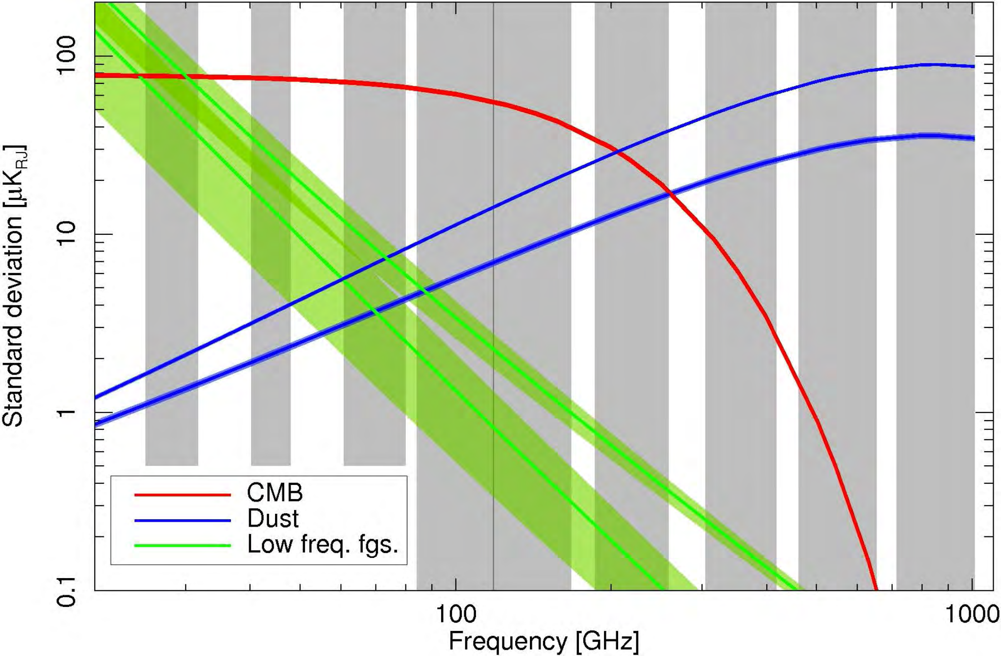
In the 2013 data release, we adopt the posterior mean as our signal estimate, and the posterior RMS as the corresponding uncertainty. Mean and RMS maps are provided for each signal component and for each per-pixel spectral parameter. Two caveats are in order regarding use of these products for further scientific analysis. First, significant systematic uncertainties are associated with several of these estimates. One example is the correlated HFI noise that is seen clearly in the thermal dust emissivity map; the products presented here do not take into account spatially correlated noise. Second, the full posterior is significantly non-Gaussian due to the presence of non-Gaussian spectral parameters and the positivity amplitude prior, as well as strongly correlated between components. The mean and RMS maps provided in this data release should therefore be understood as a convenient representation of the full posterior, rather than a precise description of each component; if very high statistical precision is required, one should use instead the original ensemble of individual Monte Carlo samples.

8.2.2 Thermal emission from Galactic dust
The CMB fades toward higher frequencies, whereas the thermal dust emission spectrum increases, and so dust becomes the dominant signal at submillimetre wavelengths. Planck has multifrequency sensitivity in the “dust channels” covering the spectral range where this transition occurs up to 857 GHz, for which the angular resolution is highest (Table 2). Dust emission is seen extending to high Galactic latitude in the wispy “cirrus” represented in bluish tones in Fig. 1.
Understanding the frequency dependence and spatial fluctuations of the intensity and polarization from thermal dust is important both in separating this foreground from the CMB and as an all-sky measure of column density. This has motivated the development of the Planck dust model (Planck Collaboration XI 2014; Fig. 22). The use of a range of available ancillary data distinguishes this model from the dust component extracted using component separation techniques and frequencies below 353 GHz, described in Sect. 8.2.1.
The Planck dust model is based on the maps at 353, 545, and 857 GHz, plus the IRAS 100 m (3000 GHz) data from the IRIS product (Miville-Deschênes & Lagache 2005). As described in Planck Collaboration VI (2014), the zero level of these maps can be set such that there is no dust emission where there is no atomic H i gas column density (according to the LAB survey, Kalberla et al. 2005).
The dust temperature is determined by multi-frequency fitting of a greybody SED for optically thin thermal dust, , where is the dust optical depth of the column of material and is the Planck function for . In the Planck dust model there are three parameters, , at 353 GHz, and , the exponent of the assumed power-law frequency dependence of . Conversion of to is established by correlating the submillimetre optical depth with SDSS reddening measurements of quasars, a very similar approach to the one adopted by Schlegel et al. (1998).
All-sky maps of and from Planck were first presented by Planck Collaboration XIX (2011) using a fixed . In the new Planck dust model (Planck Collaboration XI 2014), the maps of and are at 5′ resolution, while is estimated at 35′. This provides a much more detailed description of the thermal dust emission than the Finkbeiner et al. (1999) model, which assumed constant and used a map with an angular resolution of several degrees.
The high resolution of Planck is a major improvement that results in a much more detailed mapping of column density structure, especially in denser regions of the ISM where the equilibrium temperature of big dust grains changes on small angular scales due to attenuation of the radiation field and also, it appears, to changes in the intrinsic dust opacity and its ability to emit. Because of the increase in sensitivity, better control of systematic effects, and the combination of four intensity maps at 5′ resolution spanning the peak of the SED and into the Rayleigh-Jeans region, the new Planck product also provides a precise estimate of the dust column density even in the diffuse ISM where does not vary as strongly on small scales.
8.2.3 Polarized emission from Galactic dust
As described in Sect. 1.3, Planck polarization data are in a less mature state than temperature data, especially at low multipoles. Nevertheless, strong polarized synchrotron and thermal dust emission from the Galaxy can already be imaged with high significance. A first set of Galactic polarization papers will be published shortly. These papers will report results on the degree of dust polarization () over the whole sky, comparisons with maps of synchrotron polarization and Faraday rotation, the structure of the Galactic magnetic field and its coupling with interstellar matter, as well as turbulence in the diffuse interstellar medium (ISM). With an angular resolution of 5′, the maps also reveal the magnetic field structure in molecular clouds and star forming regions, and can be used to study which grains contribute to the observed polarization, where in the ISM they are aligned with the Galactic magnetic field, and with what efficiency.
One highlight from these maps is the high degree of polarization of the dust emission from the diffuse interstellar medium, in many locations reaching at 353 GHz. These studies will also address the statistics of and for selected fields towards nearby molecular clouds (e.g., Fig. 26), the relationship with MHD simulations, the spectral dependence of the polarized emission, and a comparison of the degree of polarization at submillimetre and visible (from stellar observations) wavelengths.
8.2.4 CO extraction
Rotational line emission from carbon monoxide (CO) in the interstellar medium is present in all HFI bands except 143 GHz, most significantly from the =10 (115 GHz), =21 (230 GHz), and =32 (345 GHz) transitions. CO emission arises from the denser parts of the interstellar medium, and is concentrated at low and intermediate Galactic latitudes. Three approaches to estimating CO emission have been evaluated and are described in Planck Collaboration XIII (2014).
Type 1 maps rely on the fact that each bolometer has a different responsivity to CO, largely due to its specific bandpass shape. The transmission at the CO transition frequency has been accurately measured on the ground, and can also be estimated by comparison to surveys made with dedicated observatories. Knowledge of the relative bolometer spectral response allows extraction of each CO line independently of the others and of any ancillary data. Being extracted from single-bolometer data, these maps have relatively low SNR; however, they are not affected by contamination from other channels, and thus can be used for unbiased removal of CO from frequency maps.
Type 2 maps are obtained using a multi-frequency component separation approach. Three maps are combined to extract independently maps of the =10 (100, 143, and 353 GHz channels) and =21 (143, 217, and 353 GHz channels) emission. Because channels are combined, the spectral behaviour of other foregrounds (free-free and dust) is needed as extra constraints to allow clean CO extraction. The Type 2 maps have higher SNR than the Type 1 maps, at the cost of residual contamination from other diffuse foregrounds. These maps constitute a unique product for astrophysics that provides the excitation ratio for all parts of the sky where the CO intensity is strong enough.
The Type 3 map is determined by fixing the =21/=10 and =32/=21 line ratios. The map is extracted using the full Commander-Ruler component separation pipeline (Sect. 8.2.1). This yields a map of combined CO emission with very high SNR that can be used as a sensitive finding chart for low-intensity diffuse CO emission over the whole sky. The line ratios can be determined from ground-based observations, or from a first iteration of the component separation algorithm with simplified assumptions; the latter is the route used by Planck.
All three types of CO map have been extensively cross-checked internally.
8.2.5 All-sky Sunyaev-Zeldovich emission
Using specialized component separation methods on Planck maps from 100 to 857 GHz, we have constructed an all-sky map that includes an estimate of the Compton parameter from the thermal Sunyaev-Zeldovich (tSZ) effect (Sunyaev & Zeldovich 1972). The angular power spectrum of this map, corrected for residual foregrounds, gives the first estimate of the tSZ power spectrum over a range of multipoles from to (Planck Collaboration XXI 2014). Diffuse thermal dust emission is the major foreground contaminant in the map at low multipoles (); at high multipoles () the clustered CIB and unresolved radio and infrared point sources dominate. At intermediate scales the tSZ dominates. The measured tSZ spectrum is composed of the total signal from resolved clusters in the Planck catalogue of SZ sources and from unresolved clusters of galaxies and hot diffuse gas (Sect. 9.7).
The tSZ Compton parameter map is not released as a product to the community because of the complexity of the foreground contamination, which does not allow for direct use without a companion foreground model.
8.3 Unresolved foregrounds at high galactic latitudes
In this section we summarize our understanding of unresolved foregrounds at high galactic latitudes, largely determined by Planck and described in previous sections. Figure 27 shows the total level of foregrounds as a fraction of the rms amplitude of CMB fluctuations over 56 % of the high-galactic-latitude sky (the mask used is G56, defined in Planck Collaboration XV (2014)). The foregrounds included are:
- •
Galactic thermal dust emission as modelled in Planck Collaboration Int. XVII (2014, see also Sect. 8.2.2 and ). The angular power spectrum is based on the 353 GHz map, from which the SMICA CMB has been subtracted, and has an dependence. The SED of this component includes Anomalous Microwave Emission, which is determined by correlation with thermal dust.
- •
Free-free emission as modelled in Planck Collaboration Int. XVII (2014). The angular power spectrum is normalized at 100 GHz, and has an and dependence.
- •
Synchrotron emission based on the Haslam 408 MHz template, with .
- •
The Cosmic Infrared Background as determined in Planck Collaboration XXX (2014, see also Sect. 9.5), extrapolated analytically for 50 and 100 GHz.
- •
Diffuse SZ emission, as modelled in Planck Collaboration XXI (2014, see also Sect. 9.7).
- •
Poisson noise from unresolved radio sources, based on the Planck PCCS at 100 GHz with a flux density threshold of 256 mJy, extrapolated in frequency as .
- •
Poisson noise from dusty galaxies based on the CIB model of Planck Collaboration XXX (2014).
Figure 28 shows two representative cuts through Fig. 27, at 100 GHz and , close to where foregrounds are least important relative to the CMB (see Fig. 27). These figures show that at the lowest and highest CMB frequencies (70 and 217 GHz), diffuse Galactic foregrounds dominate at low-, with a minimum in the 70 to 100 GHz range for the best half of the sky (see Figs. 25 and 27). Residual extragalactic foregrounds, composed of synchrotron emission from radio sources, SZ emission from clusters, and thermal dust emission from galaxies, have a more complicated behaviour in and frequency, as they contain Poisson terms and, for SZ and the CIB, correlated terms as well. Over 60 % of the sky, extragalactic foregrounds dominate at all multipoles larger than 200. The frequency at which we find the minimum relative contribution of all foregrounds with respect to the CMB shifts from 70 GHz at to larger than 100 GHz at 200 (with less than 1 % contamination up to ).
9 Planck 2013 cosmology results
9.1 Parameter estimation, lensing, and inflation
Since their discovery, anisotropies in the CMB have contributed significantly to defining our cosmological model and measuring its key parameters. The standard model of cosmology is based upon a spatially flat, expanding Universe whose dynamics are governed by General Relativity and dominated by cold dark matter and a cosmological constant (). The seeds of structure have Gaussian statistics and form an almost scale-invariant spectrum of adiabatic fluctuations.
Planck’s measurements of the cosmological parameters derived from the nominal mission are presented and discussed in Planck Collaboration XVI (2014). The most important conclusion from this paper is the excellent agreement between the Planck temperature spectrum at high and the predictions of the CDM model. All of our current observations can be fit remarkably well by a six parameter CDM model (see Table 9 for definitions), and we provide strong constraints on deviations from this model. The best-fit cosmological parameters are not affected by foreground modeling uncertainties, and the best-fit model provides an excellent fit to the spectra from Planck, ACT, and SPT (see Fig. 29). The ACT and SPT spectra are from Calabrese et al. (2013).
|
In some cases we find significant changes compared to previous CMB experiments, as discussed in detail in Planck Collaboration XVI (2014). In particular, when we compare models based on CMB data only we find that the Planck best-fit model retrieves lower (by 6 %), higher (by 9 %), and higher (by 18 %) than the corresponding WMAP91313 13 We compare the model [Planck +WP+highL] of Table 5 in Planck Collaboration XVI (2014) with [WMAP+eCMB] of Table 4 of Hinshaw et al. (2013). model. However, when adding BAO to both sets of data, the gap reduces by a factor of 3 in all three components.
Among the constraints that we determine, several are notable. The angular size of the acoustic scale is determined to , as , which leads to a constraint in the subspace for CDM models (Planck Collaboration XVI 2014, all confidence intervals are ;). For CDM, the matter and baryon densities are well determined, with the latter being consistent with recent results from big-bang nucleosynthesis (BBN). We find excellent consistency with BBN even in extensions to the six-parameter model. The predictions of the baryon density from these two methods involve all of the known forces of nature, and this highly non-trivial consistency provides strong evidence for the universality of those laws.
Lensing of the CMB enters the Planck parameter estimation results discussed in Planck Collaboration XVI (2014) in two ways. First, the power spectrum of the temperature anisotropies is modified at the few percent level by lensing, with the primary effect being a smoothing of the acoustic peaks on angular scales relevant for Planck. We detect this smoothing effect at , and include it in our parameter constraints. Second, the measurements of the power spectrum of the reconstructed gravitational lensing potential, described in Planck Collaboration XVII (2014) and Sect. 7.2, can be combined with the main Planck likelihood developed in Planck Collaboration XV (2014) (see also Sect. 7.3). The lensing power spectrum measurements condense the cosmological signal contained in the non-Gaussian 4-point function of the CMB anisotropies in a near-optimal way. Combining the lensing likelihood with the main Planck likelihood is therefore equivalent to a joint analysis of the anisotropy power spectrum and that part of the 4-point function due to lensing.
The expected lensing power spectrum is tightly constrained in the six-parameter CDM model by the Planck temperature power spectrum and the WMAP low- polarization data. The best-fitting model predicts a lensing power spectrum in good agreement with the Planck lensing reconstruction measurement, further validating the predictions of the CDM model, calibrated on the CMB fluctuations at . These predictions include clustering and the evolution of the geometry at low redshift. We express the amplitude of the lensing power spectrum in terms of a phenomenological power spectrum amplitude parameter, , which scales the theoretical 4-point function (due to lensing) at each point in parameter space. From Planck’s best-fit model, the expected value of this scaling parameter is 1.0; for the nominal mission we find (68 % CL; Planck Collaboration XVI 2014).
Without the low- polarization data, and in the absence of lensing, the amplitude of the primordial power spectrum, , and the optical depth to reionization, , would be degenerate with only the combination being well determined by the (unlensed) temperature power spectrum. However, lensing partially breaks this degeneracy, since the lensing power spectrum is independent of the optical depth. Combining the temperature power spectrum with the lensing likelihood, we determine (68 % CL) from the temperature anisotropies alone. This constraint is consistent, though weaker, than that from WMAP polarization (Hinshaw et al. 2012a). Importantly, the lensing route does not depend on the challenging issue of removing large-scale polarized emission from our Galaxy that is critical for the WMAP measurement. At 95 % confidence, we can place a lower limit on the optical depth , which exceeds the value for instantaneous reionization at , further supporting the picture that reionization is an extended process.
Beyond the six-parameter CDM model, the Planck lensing measurements strengthen the evidence reported by ACT (Sievers et al. 2013) and SPT (van Engelen et al. 2012; Story et al. 2012) for dark energy from the CMB alone in models with spatial curvature. Closed models with low energy density in dark energy can be found that produce unlensed CMB power spectra nearly identical to the best-fitting CDM model. This “geometric” degeneracy is partially broken by lensing, since the closed models predict too much lensing power. Even without using the Planck lensing reconstruction, the detection of the smoothing of the temperature power spectrum allows Planck, used in combination with ACT and SPT at high- (to better constrain extragalactic foregrounds) and WMAP large scale polarization, to break the geometrical degeneracy, and provides evidence for dark energy purely from the CMB (Planck Collaboration XVII 2014). Adding the lensing likelihood, we constrain any departures from spatial flatness at the percent level: (68 % CL) for the same data combination, improving earlier CMB-only constraints (Story et al. 2012) by around a factor of two, and setting our determination of dark energy from temperature anisotropies data alone to (68 % CL). Tighter constraints from the combination of Planck and other astrophysical data are given in Planck Collaboration XVI (2014).
Within the minimal, six-parameter model the expansion rate is well determined, independent of the distance ladder. One of the most striking results of the nominal mission is that the best-fit Hubble constant , is lower than that measured using traditional techniques, though in agreement with that determined by other CMB experiments (e.g., most notably from the recent WMAP9 analysis where Hinshaw et al. 2012b find consistent with the Planck value to within ). Freedman et al. (2012), as part of the Carnegie Hubble Program, use mid-infrared observations with the Spitzer Space Telescope to recalibrate secondary distance methods used in the HST Key Project. These authors find where the first error is statistical and the second systematic. A parallel effort by Riess et al. (2011) used the Hubble Space Telescope observations of Cepheid variables in the host galaxies of eight SNe Ia to calibrate the supernova magnitude-redshift relation. Their ‘best estimate’ of the Hubble constant, from fitting the calibrated SNe magnitude-redshift relation is, where the error is and includes known sources of systematic errors. At face value, these measurements are discrepant with the current Planck estimate at about the level. This discrepancy is discussed further in Planck Collaboration XVI (2014).
Extending the Hubble diagram to higher redshifts, we note that the best-fit CDM model provides strong predictions for the distance scale. This prediction can be compared to the measurements provided by studies of Type Ia SNe and baryon acoustic oscillations (BAO). Driven in large part by our preference for a higher matter density, we find mild tension with the (relative) distance scale inferred from compilations of SNe (Conley et al. 2011; Suzuki et al. 2012). In contrast our results are in excellent agreement with the BAO distance scale compiled in Anderson et al. (2012) covering the redshift range 0.1 to 0.7.
|
||||||||||||||||||||||||||||||||||||||||||||||||||||||||||||||||||||||||||||||||||
The Planck data, in combination with polarization measured by WMAP, high- anisotropies from ACT and SPT and other, lower redshift data sets, provide strong constraints on deviations from the minimal model. The low redshift measurements provided by BAO allow us to break some degeneracies still present in the Planck data and significantly tighten constraints on cosmological parameters in these model extensions. The ACT and SPT data help to fix our foreground model at high . The combination of these experiments provides our best constraints on the standard 6-parameter model; values of some key parameters in this model are summarized in Table 10.
From an analysis of an extensive grid of models, we find no strong evidence to favour any extension to the base CDM cosmology, either from the CMB temperature power spectrum alone or in combination with the Planck lensing power spectrum and other astrophysical datasets. For the wide range of extensions that we have considered, the posteriors for extra parameters generally overlap the fiducial model within . The measured values of the CDM parameters are relatively robust to the inclusion of different parameters, though a few do broaden significantly if additional degeneracies are introduced. When the Planck likelihood does provide marginal evidence for extensions to the base CDM model, this comes predominantly from a deficit of power (compared to the base model) in the data at .
The primordial power spectrum is well described by a power-law over three decades in wave number, with no evidence for “running” of the spectral index. The spectrum does, however, deviate significantly () from scale invariance, as predicted by most models of inflation (see below). The unique contribution of Planck, compared to previous experiments, is that the departure from scale invariance is robust to changes in the underlying theoretical model.
We find an effective number of neutrino-like relativistic degrees of freedom of , compatible with the standard value of 3.046, implying no need for extra relativistic species beyond the three species of (almost) massless neutrinos and photons. The main effect of massive neutrinos is a suppression of clustering on scales larger than the horizon size at the non-relativisitic transition. This affects both , with a damping for , and , reducing the lensing-induced smoothing of the acoustic peaks. Using Planck data in combination with polarization measured by WMAP and high- anisotropies from ACT and SPT allows for a constraint of (95 % CL) based on the [Planck+WP+highL] model. Curiously, this constraint is weakened by the addition of the lensing likelihood (95 % CL), reflecting mild tensions between the measured lensing and temperature power spectra, with the former preferring larger neutrino masses than the latter. Possible origins of this tension are explored further in Planck Collaboration XVI (2014) and are thought to involve both the measurements and features in the measured on large scales () and small scales that are not fit well by the CDM+foreground model. The SNR on the lensing measurement will improve with the full mission data, including polarization, and it will be interesting to see how this story develops.
The combination of large lever arm, sensitivity to isocurvature fluctuations, and non-Gaussianity makes Planck particularly powerful at probing inflation. The constraints on inflationary models are presented in Planck Collaboration XXII (2014) and are consistent with a single, weakly coupled, neutral scalar field driving the accelerated expansion and generating curvature perturbations. The data can be explained using a field with a canonical kinetic term and slowly rolling down a featureless potential, and we find no compelling evidence calling for any extension to this simple explanation.
Of the models considered, those with locally concave potentials are favored and occupy most of the region in the - plane allowed at 95 % confidence level (see Fig. 30). Power law inflation, hybrid models driven by a quadratic term, and monomial large field potentials with a power larger than two lie outside the 95 % confidence contours. The quadratic large field model, in the past often cited as the simplest inflationary model, is now at the boundary of the 95 % confidence contours of Planck + WP + CMB high data.

The axion and curvaton scenarios, in which the CDM isocurvature mode is uncorrelated or fully correlated with the adiabatic mode, respectively, are not favored by Planck, which constrains the contribution of the isocurvature mode to the primordial spectra at Mpc-1 to be less than 3.9 % and 0.25 % (95 % CL), respectively.
The Planck results come close to the tightest upper limit on the tensor-to-scalar amplitude possible from temperature data alone. The precise determination of the higher acoustic peaks breaks degeneracies that have weakened earlier measurements. The bound ( at 95 % CL) implies an upper limit for the energy scale of standard inflation of GeV (95 %CL).
The power spectrum of the best fit base CDM cosmology has a higher amplitude than the observed power spectrum at multipoles . The low- difference is in turn related to the preference for a higher lensing amplitude when fitting to the temperature anisotropy power spectrum through a chain of parameter degeneracies (see Planck Collaboration XVI 2014, for discussion). There are other indications for ‘anomalies’ at low (Sect. 9.2, Planck Collaboration XXIII (2014)), which may be indicative of new physics operating on the largest scales; however, the interpretation of such anomalies is difficult in the absence of a compelling theoretical framework. In addition, our determination of the power spectrum amplitude is in weak tension with that derived from the abundance of rich clusters found with the Sunyaev-Zeldovich effect in the Planck data (Planck Collaboration XX 2014) and from measurements of cosmic shear from the CFHTLenS survey (Heymans et al. 2012; Erben et al. 2012).
9.2 Isotropy and Gaussianity
Two of the fundamental assumptions of the standard cosmological model, that the initial fluctuations are statistically isotropic and Gaussian, are rigorously examined in Planck Collaboration XXIII (2014) and Planck Collaboration XXIV (2014), using the four CMB maps described in Sect. 7.1. Realistic simulations incorporating essential aspects of the Planck measurement process have been used to support the analysis. Deviations from isotropy have been found in the data that are robust against changes in the component separation algorithm or mask used, or the frequency examined. Many of these anomalies were previously observed in the WMAP data on large angular scales (e.g., an alignment between the quadrupole and octopole moments, an asymmetry of power between two preferred hemispheres, and a region of significant decrement, the so-called Cold Spot), and are now confirmed at similar levels of significance () but a higher level of confidence. In spite of the presence of strong non-Gaussian and anisotropic emission coming from Galactic and extragalactic sources, the consistency of the tests performed on the four CMB maps produced by the component separation algorithms strongly favors a cosmological origin for the anomalies. Moreover, the agreement between WMAP and the two independent instruments of Planck argues against possible explanations based on systematic artifacts.
On the other hand, we find little evidence for non-Gaussianity, with the exception of a few statistical signatures that seem to be associated with specific anomalies. In particular, we find that the quadrupole-octopole alignment is also connected to a low observed variance of the CMB signal with respect to the standard CDM model. In addition, the hemispherical asymmetry is now found to persist to smaller angular scales, and can be described in the low- regime at a statistically significant level by a phenomenological dipole modulation model. It is plausible that some of these features may be reflected in the angular power spectrum of the data, which shows a deficit of power on these scales. Indeed, when the two opposing hemispheres defined by the preferred direction are considered separately, the power spectrum shows a clear power asymmetry, as well as oscillations between odd and even modes that may be related to parity violation and phase correlations also detected in the data. While these analyses represent a step forward in building an understanding of the anomalies, a satisfactory explanation based on physically motivated models is still lacking.
The search for specific types of non-Gaussianity (NG) in the statistics of the CMB anisotropies provides important clues to the physical origin of cosmological perturbations. Indeed, perturbations generated during inflation are expected to display specific forms of NG. Different inflationary models, firmly rooted in modern theoretical particle physics, predict different amplitudes and shapes of NG. Thus, constraints on primordial NG are complementary to constraints on the scalar spectral index of curvature perturbations and the tensor-to-scalar ratio, lifting the degeneracy among inflationary models that predict the same power-spectra. The level of NG predicted by the simplest models of inflation, consisting of a single slowly-rolling scalar field, is low and undetectable even by Planck. However, extensions of the simplest paradigm generically lead to levels of NG in CMB anisotropies that should be detectable. A detection of primordial NG would rule out all canonical single-field slow-roll models of inflation, pointing to physics beyond the simplest inflation model. Conversely, a significant upper bound on the level of primordial NG, as we have obtained, severely limits extensions of the simplest paradigm.
Inflationary NG can be characterized by the dimensionless non-linearity parameter (Planck Collaboration XXIV 2014), which measures the amplitude of primordial NG of quadratic type in the comoving curvature perturbation mode. We have estimated for various NG shapes, including the three fundamental ones, local, equilateral, and orthogonal, predicted by different classes of inflationary models. Results for these three fundamental shapes, obtained using a suite of optimal bispectrum estimators (Planck Collaboration XXIV 2014), are reported in Table 11, which gives independent estimates for each contribution. The reported values have been obtained after marginalizing over the Poisson bispectrum contribution of diffuse point-sources and subtracting the bias due to the secondary bispectrum arising from the coupling of the Integrated Sachs-Wolfe effect (ISW; Sect. 9.4) and the weak gravitational lensing of CMB photons (Planck Collaboration XIX 2014). We also obtain constraints on key, primordial, non-Gaussian paradigms, including non-separable single-field models, excited initial states (non-Bunch-Davies vacua), and directionally-dependent vector field models, and we provide an initial survey of scale-dependent features and resonance models. The absence of significant non-Gaussianity implies that the speed of sound of the inflaton field in these models must be within two orders of magnitude of the speed of light.
Moreover, we derive bispectrum constraints on a selection of specific inflationary mechanisms, including both general single-field inflationary models and multifield ones. Our results lead to a lower bound on the speed of sound, ( CL), in the effective field theory parametrization of the inflationary model space. Moving beyond the bispectrum, Planck data also provide an upper limit on the amplitude of the trispectrum in the local NG model, ( CL).
The Planck data have been used to provide stringent new constraints on cosmic strings and other defects (Planck Collaboration XXV 2014). Using CMB power-spectrum forecasts for cosmic strings, we obtain new limits for Nambu strings and for field theory strings. Tighter constraints for joint analysis with high- data are also described, along with results for textures and semi-local strings. Complementary non-Gaussian searches using different methodologies also find no evidence for cosmic strings, with somewhat weaker constraints.
Alternative geometries and non-trivial topologies have also been analyzed (Planck Collaboration XXVI 2014). The Bianchi VIIh models, including global rotation and shear, have been constrained, with the vorticity parameter (95 % CL). Topological models are constrained by the lack of matched circles or other evidence of large-scale correlation signatures, limiting the scale of the fundamental domain to the size of the diameter of the scattering surface in a variety of specific models.
|
||||||||||||||
9.3 CMB polarization
The current data release and scientific results are based on temperature data only. Planck measures polarization from 30 to 353 GHz, and both DPCs routinely produce polarization products. The analysis of polarization data is more complicated than that of temperature data: there are few celestial polarization sources that can be used for calibration; polarized astrophysical foregrounds dominate the polarized CMB over the whole sky; and the detection of polarized signals is subject to specific systematic effects, such as leakage of total intensity into polarization through calibration errors between detectors in a polarized pair.
These issues are not yet resolved at a level satisfactory for cosmological analysis at large angular scales (100). At smaller angular scales and high Galactic latitudes, however, systematic effects are sub-dominant, and CMB polarization is already being measured by Planck with unprecedented sensitivity. Moreover, strong polarized synchrotron and thermal dust emission from the Galaxy are currently being imaged with high significance (Sect. 8.2.3).
Planck’s ability to measure polarization is well illustrated by the use of stacking around CMB peaks (Fig. 31; compare with Hinshaw et al. 2013). Adiabatic scalar fluctuations result in a specific polarization pattern around cold and hot spots. We degrade ILC estimates (100–353 GHz; Eriksen et al. 2004) of the CMB , , and maps to HEALPix and smooth to 30′. On the 71 % of the sky outside the Planck component separation mask (Planck Collaboration XII 2014), we find 11 396 cold spots and 10 468 hot spots, consistent with the CDM Planck best fit model prediction of each. Around each of these temperature extrema, we extract square maps, which are stacked. The stacked and maps are rotated in the temperature extrema radial frame and (Kamionkowski et al. 1997). In this reference frame the standard model predicts alternating between positive (radial polarization) and negative (tangential polarization) values and (Baccigalupi 1999).

Figure 31 compares stacked and maps for cold and hot spots computed from the Planck data with those computed from the Planck best-fit CDM model. The data are in excellent agreement with the best-fit model. The combined best fit amplitude is (68 % CL), a detection with a statistical significance greater than 95.
The most interesting cosmological signal visible in polarization is the very large-scale () -mode peak due to reionization, at a typical brightness level well below one microkelvin. At the present stage of analysis, and with the data currently available, there are unexplained residuals in the Survey-to-Survey difference maps that are comparable to or larger than this. For these reasons, we are delaying the use of CMB polarization measurements from Planck for cosmological analysis until we have firmer understanding and control of such systematic effects.
9.4 The ISW effect
In the spatially flat Universe established by Planck, the detection of the integrated Sachs-Wolfe (ISW) effect provides complementary evidence of the accelerated expansion of the Universe governed by some form of Dark Energy. The high sensitivity, high resolution, and full-sky coverage of Planck has permitted us, for the first time, to obtain evidence of the ISW directly from CMB measurements, via the non-Gaussian signal induced by the cross-correlation of the secondary anisotropies due to the ISW itself and the lensing clearly detected by Planck (Planck Collaboration XVII 2014). Following this approach, we report an ISW detection of from the CMB alone.
In addition, we have also confirmed (Planck Collaboration XIX 2014) the ISW signal by cross-correlating the clean CMB maps produced by Planck with several galaxy catalogues, which act as tracers of the gravitational potential. Combining information from all the Surveys, this standard technique provides an overall detection of . This figure is somewhat weaker than previous claims made from WMAP data (Ho et al. 2008; Giannantonio et al. 2012, e.g.,). Differences do not seem to be related to the CMB data itself, but rather to the way in which the uncertainties are computed and, especially, to the characterization of the galaxy catalogues. A small fraction of these differences (around 0) may be due to the different cosmological models determined by each experiment, in particular, the lower values of and reported by Planck. Clear agreement with previous detection claims () using the NVSS data is reported. The ISW amplitude estimation made with Planck is in good agreement with the theoretical expectation (which depends on such characterizations), whereas deviations of more than were found in previous work. These results give support and robustness to our findings.
The ISW signal induced by isolated features in the large-scale structure of the universe has also been studied. In particular, we stacked CMB fluctuations at the positions of voids and super-clusters, obtaining a clear detection ( and almost for voids and clusters, respectively) of a secondary anisotropy. The results are compatible with previous claims made with WMAP data (Granett et al. 2008), and the most likely origin of the secondary anisotropy is the time evolution of the gravitational potential associated with those structures. However, the signal initially detected is at odds in scale and amplitude with expectations of a pure ISW effect. Using more recent void catalogues leads to the detection of a signal at up to with scales and amplitudes more consistent with expectations of the ISW effect. Taking advantage of the large frequency coverage of Planck, we have confirmed that the stacked signal is stable from 44 to 353 GHz, supporting the cosmological origin of this detection.
9.5 The cosmic infrared background
CIB anisotropies are expected to trace large-scale structures and probe the clustering properties of galaxies, which in turn are linked to those of their host dark matter halos. Because the clustering of dark matter is well understood, observations of anisotropies in the CIB constrain the relationship between dusty, star-forming galaxies and the dark matter distribution. Correlated anisotropies also depend on the mean emissivity per comoving unit volume of dusty, star-forming galaxies, and can be used to measure the star formation history.
The extraction of CIB anisotropies in Planck (Planck Collaboration XVIII 2011; Planck Collaboration XXX 2014) is limited by our ability to separate the CIB from the CMB and Galactic dust. At multipole =100, the power spectrum of the CIB anisotropies has an amplitude less than 0.2 % of the CMB power spectrum at 217 GHz, and less than 25 % of the dust power spectrum in very diffuse regions of the sky ( cm-2) at 857 GHz. Using H i data from three radio telescopes (Parkes, GBT, and Effelsberg) and cleaning the CMB using the 100 GHz map as a template, it has been possible to obtain new measurements of the CIB anisotropies with Planck. The CIB has been extracted from the maps on roughly 2300 deg2 (Planck Collaboration XXX 2014). Auto- and cross-power spectra have been computed, from 143 to 3000 GHz, using both Planck and IRAS. Two approaches have been developed to model the power spectra. The first uses only the linear part of the clustering and gives strong constraints on the evolution of the star formation rate throughout cosmic time. The second is based on a parameterized relation between the dust-processed infrared luminosity and (sub-)halo mass, and probes the interplay between baryonic and dark matter up to very high redshifts, complementing current and foreseeable optical or near-infrared measurements.
The CIB, not the CMB, is the dominant extragalactic signal at 857 and 545 GHz, and even at 353 GHz for . Comprising redshifted thermal radiation from ultraviolet-heated dust enshrouding young stars, the CIB contains much of the energy from processes involved in structure formation. According to current models, the dusty star-forming galaxies that give rise to the CIB have a redshift distribution peaked between and , and tend to live in – dark matter halos. At all redshifts, the dominant contribution to the SFR density is from halos of mass .
9.6 Lensing and the cosmic infrared background
Planck’s multi-frequency observations provide information on both the integrated history of star formation via the CIB and the distribution of dark matter via CMB lensing.
Gravitational lensing by large-scale structure produces small shear and magnification effects in the observed fluctuations, which can be exploited to reconstruct an integrated measure of the gravitational potential along the line of sight. This “CMB lensing potential” is sourced primarily by dark matter halos located at , roughly halfway between ourselves and the last scattering surface.
The conjunction of these two unique probes allows us to measure directly the connection between dark and luminous matter in the high redshift () Universe (Planck Collaboration XVIII 2014). We use a three-point statistic optimized to detect the correlation between these two tracers, and report the first detection of the correlation between the CIB and CMB lensing using Planck data only. The well-matched redshift distribution of these two signals leads to a detection significance with a peak value of at 545 GHz. Equivalently, we measure a correlation as high as 80 % across these two tracers. Our full set of multi-frequency measurements (both CIB auto- and CIB-lensing cross-spectra) is consistent with a simple halo-based model, with the mean halo mass that is most efficient at hosting star formation being . Leveraging the frequency dependence of our signal, we isolate the high redshift contribution to the CIB, and constrain the star formation rate (SFR) density at . We measure directly the SFR density with around 4 significance for three redshift bins between and 7, thus opening a new window into the study of the formation of stars at early times.

Figure 32 shows the real-space correlation between the observed temperature and the lens deflection angles. This figure allows us to visualize the correlation between the CIB and the CMB lensing deflection angles for the first time. These images were generated using a stacking technique, as described in Planck Collaboration XVIII (2014). We select 20 000 local maxima and an equal number of local minima, stack them in one-degree squares, then take the gradient of the stacked lensing potential to calculate the deflection angles, shown in the figure as arrows. The result of stacking over the maxima, minima, and random points is displayed from left to right. The strong correlation seen already in the cross-power spectrum is clearly visible in both the 545 and 857 GHz extrema, while stacking on random locations leads to a lensing signal consistent with noise. As expected, we see that the temperature maxima of the CIB, which contain a larger-than-average number of galaxies, deflect light inward, i.e., they correspond to gravitational potential wells, while temperature minima trace regions with fewer galaxies and deflect light outward, i.e., they correspond to gravitational potential hills.
9.7 Cosmology from Planck Sunyaev–Zeldovich emission
Clusters of galaxies are good tracers of the evolution and content of the Universe. (Planck Collaboration XX 2014) gives constraints obtained with a well defined sample of 189 clusters (Sect. 8.1.2) for which we have computed the selection function. This sample has to ensure 100 % reliability and to maximize the number of redshifts (188). Using a relation between mass and SZ signal based on comparison to X-ray measurements, we derive constraints on the matter power spectrum amplitude and matter density parameter in a flat CDM model. Assuming a bias between the X-ray determined mass and the true mass in the range 0–30 %, motivated by comparison of the observed mass scaling relations to those from several sets of numerical simulations, we find that , with one dimensional ranges and . This result appears to be robust against the SNR cut, choice of sub-sample, mass function, or completeness assumptions.
In addition to the above analysis based on cluster counts, we can derive cosmological constraints from the power spectrum of tSZ emission (see Sect. 8.2.5, and Planck Collaboration XXI 2014). We have compared the Planck angular power spectrum of the diffuse thermal SZ emission (tSZ) to theoretical models in order to set cosmological constraints. The two analyses exhibit a similar degeneracy relation between and . In particular, we measure , with one-dimensional ranges and , in agreement with the constraints derived from SZ cluster counts.
The tSZ effect secondary anisotropies are expected to be non-Gaussian, thus extra and independent cosmological information can be extracted from the higher-order moments of their distribution and from their bispectrum. By computing the one-dimensional probability distribution function of the tSZ map, we find , compatible with the bispectrum-based estimate of .
While these analyses show good consistency on the constraints from the SZ signal detected by Planck (and with other cluster measurements), they favour somewhat low values of and as compared to the CMB analysis (Sect. 9.1). This tension can be alleviated either by relaxing our assumption on the bias between X-ray mass and true mass, or by assuming massive neutrinos. Although additional neutrino species are not required by analysis of fluctuations in the CMB (Sect. 9.1, the upper limits on given there do not rule out additional massive neutrinos at a level that would reduce the tension in and .
10 Summary and Conclusions
We have summarized the data products and scientific results of Planck’s first 15.5 months of science operations. Full descriptions of all aspects of the Planck data analysis and science results in this 2013 release are given in the accompanying papers (Planck Collaboration 2013 II – XXXI).
Planck has been a tremendous technical success. The satellite and its complex cryogenic payload have operated without interruption over a lifetime longer than initially planned by a factor of three, with payload performance as good as or better than expected from pre-launch ground testing.
The 2013 data release fulfills the promise made at mission inception in 1995 by delivering: (a) a set of nine well-characterized frequency maps with sub-percent calibration accuracy across the CMB channels; (b) a map of the temperature anisotropies of the CMB limited only by unresolved foregrounds down to an angular resolution of 5′; (c) a catalogue of compact Galactic and extragalactic sources that represents an important improvement over the Early Release Compact Source Catalogue released in January 2011; (d) a catalogue of galaxy clusters detected via the Sunyaev-Zeldovich effect, which increases by a factor of 10 the number of clusters detected by this technique; and (e) a first-generation set of maps of diffuse foregrounds that includes the main sources of Galactic emission — thermal dust and the cosmic infrared background at high frequencies and synchrotron, free-free, and anomalous emission at low frequencies.
In addition to these long-planned products, the 2013 release includes: an all-sky map of dust opacity that represents an important improvement over the best previous IRAS-based product; an all-sky map of the CMB lensing deflection field, the first ever in its category; all-sky maps of the integrated emission of carbon monoxide, an important tracer of the interstellar medium; and the first measurement of the angular power spectrum of the diffuse Sunyaev-Zeldovich emission over a large part of the sky.
The main cosmological results of Planck can be summarised as follows:
- •
Using a likelihood approach that combines Planck CMB and lensing data, data from ACT and SPT at high s to constrain foregrounds, and the WMAP polarized likelihood function at low s to constrain , we have estimated the values of a six-parameter CDM model with the highest accuracy ever. These estimates are highly robust, as demonstrated by the use of multiple methods based both on likelihood and on component-separated maps.
- •
The parameters of the Planck 6-parameter CDM model are significantly different from those previously estimated. In particular, we find a weaker cosmological constant (by 2 %), more baryons (by 3 %), and more cold dark matter (by 5 %). The spectral index of primordial fluctuations is firmly established to be below unity, even when extending the CDM model with additional parameters.
- •
We find no significant improvements to the best-fit model when extending the set of parameters beyond six, implying no need for new physics to explain the Planck measurements.
- •
The Planck best-fit model is in excellent agreement with the most current BAO data. However, it requires a Hubble constant that is significantly lower (67 km s-1 Mpc-1) than that determined from traditional measurement techniques, raising the possibility of systematic effects in the latter.
- •
An exploration of parameter space beyond the basic set leads to: (a) establishing a value for the effective number of relativistic species (neutrinos) consistent with the standard value of 3.046; (b) constraining the flatness of space-time to a level of 0.1% (including BAO data); and (c) setting significantly improved constraints on the total mass of neutrinos (at ), the abundance of primordial helium, and the running of the spectral index of the power spectrum (Planck Collaboration XVI 2014).
- •
We find no evidence at the current level of analysis for tensor modes, for a dynamical form of dark energy, or for time-variations of the fine structure constant (Planck Collaboration XVI 2014).
- •
We find some tension between the amplitude of matter fluctuations () derived from CMB data and that derived from Sunyaev-Zeldovich data; we attribute this tension to uncertainties in cluster physics and measurements that affect the latter.
- •
We find important support for single-field slow-roll inflation via our constraints on running of the spectral index, curvature, and .
- •
The Planck data squeeze the region of allowed standard inflationary models, preferring a concave potential. Power law inflation, the simplest hybrid inflationary models, and simple monomial models with , do not provide a good fit to the data.
- •
We find no evidence for statistical deviations from isotropy at , to very high precision Planck Collaboration XXIII (2014).
- •
We do find evidence for deviations from isotropy at low multipoles, confirming the existence of the so-called WMAP anomalies, the hemispheric asymmetry and the Cold Spot.
- •
We find a coherent deficit of power at multipoles between 20 and 30 with respect to our best-fit CDM model.
These results highlight the maturity and precision being achieved in our understanding of the Universe, but at the same time reveal small differences between the data and the best-fit model whose significance is not yet fully understood.
Other results for which the current Planck data are making unique contributions are:
- •
A detection of the distortion of the CMB due to lensing by intervening structure yields a highly significant map over most of the sky of the integrated distribution of mass back to the CMB surface of last scattering. The detection of lensing helps Planck to break parameter degeneracies, in particular to constrain the reionization optical depth without the help of polarization data.
- •
The first detection at high significance () of the cross-correlation between CMB lensing and the cosmic infrared background, which allows us to constrain the star formation rate at high redshifts.
- •
The measurement of the angular power spectrum of the cosmic infrared background over a large area and at frequencies as low as 217 GHz, which allows us to constrain the properties of dark matter halos at high redshifts.
- •
The first power spectrum of the diffuse Sunyaev-Zeldovich emission over the range , used to constrain the amplitude of matter fluctuations ().
- •
A detection of the Integrated Sachs-Wolfe effect via its cross-correlation with Planck-detected lensing, providing independent evidence for 0.7.
The Planck 2013 release does not include polarization products. Our current cosmological analysis relies not at all on Planck polarization data, and only mildly on WMAP polarization data. However, we have shown that quite basic processing of the CMB polarization already yields angular power spectra in excellent agreement with the Planck best-fit cosmology derived from temperature data only. Analysis of the stacking of hot and cold CMB peaks shows spectacular agreement with expectations, and demonstrates the potential of the Planck’s CMB polarization measurements. A number of papers on polarized dust emission are due to be published within a few months. All these points show that the processing of Planck polarization data is well advanced, and progressing towards the goal of releasing polarized data and associated results in 2014.
Acknowledgements.
Planck is too large a project to allow full acknowledgement of all contributions by individuals, institutions, industries, and funding agencies. The main entities involved in the mission operations are as follows. The European Space Agency operates the satellite via its Mission Operations Centre located at ESOC (Darmstadt, Germany) and coordinates scientific operations via the Planck Science Office located at ESAC (Madrid, Spain). Two Consortia, comprising around 100 scientific institutes within Europe, the USA, and Canada, and funded by agencies from the participating countries, developed the scientific instruments LFI and HFI, and continue to operate them via Instrument Operations Teams located in Trieste (Italy) and Orsay (France). The Consortia are also responsible for scientific processing of the acquired data. The Consortia are led by the Principal Investigators: J.-L. Puget in France for HFI (funded principally by CNES and CNRS/INSU-IN2P3) and N. Mandolesi in Italy for LFI (funded principally via ASI). NASA’s US Planck Project, based at JPL and involving scientists at many US institutions, contributes significantly to the efforts of these two Consortia. A third Consortium, led by H. U. Norgaard-Nielsen and supported by the Danish Natural Research Council, contributed to the reflector programme. The author list for this paper has been selected by the Planck Science Team from the Planck Collaboration, and is composed of individuals from all of the above entities who have made multi-year contributions to the development of the mission. It does not pretend to be inclusive of all contributions to Planck. A description of the Planck Collaboration and a list of its members, indicating which technical or scientific activities they have been involved in, can be found at (http://www.rssd.esa.int/index.php?project=PLANCK& page=Planck_ Collaboration). The Planck Collaboration acknowledges the support of: ESA; CNES, and CNRS/INSU-IN2P3-INP (France); ASI, CNR, and INAF (Italy); NASA and DoE (USA); STFC and UKSA (UK); CSIC, MICINN, and JA (Spain); Tekes, AoF, and CSC (Finland); DLR and MPG (Germany); CSA (Canada); DTU Space (Denmark); SER/SSO (Switzerland); RCN (Norway); SFI (Ireland); FCT/MCTES (Portugal); and PRACE (EU).References
- Anderson et al. (2012) Anderson, L., Aubourg, E., Bailey, S., et al. 2012, MNRAS, 427, 3435
- Baccigalupi (1999) Baccigalupi, C. 1999, Phys. Rev. D, 59, 123004
- Bennett et al. (2003) Bennett, C. L., Halpern, M., Hinshaw, G., et al. 2003, ApJS, 148, 1
- Bennett et al. (2013) Bennett, C. L., Larson, D., Weiland, J. L., et al. 2013, ApJS, 208, 20
- Bersanelli et al. (2010) Bersanelli, M., Mandolesi, N., Butler, R. C., et al. 2010, A&A, 520, A4
- Böhringer et al. (2004) Böhringer, H., Schuecker, P., Guzzo, L., et al. 2004, A&A, 425, 367
- Böhringer et al. (2000) Böhringer, H., Voges, W., Huchra, J. P., et al. 2000, ApJS, 129, 435
- Burenin et al. (2007) Burenin, R. A., Vikhlinin, A., Hornstrup, A., et al. 2007, ApJS, 172, 561
- Calabrese et al. (2013) Calabrese, E., Hlozek, R. A., Battaglia, N., et al. 2013, ArXiv e-prints
- Cardoso et al. (2008) Cardoso, J., Martin, M., Delabrouille, J., Betoule, M., & Patanchon, G. 2008, IEEE Journal of Selected Topics in Signal Processing, 2, 735, special issue on Signal Processing for Astronomical and Space Research Applications
- Chen et al. (2013) Chen, X., Rachen, J. P., López-Caniego, M., et al. 2013, A&A, 553, A107
- Condon et al. (1998) Condon, J. J., Cotton, W. D., Greisen, E. W., et al. 1998, AJ, 115, 1693
- Conley et al. (2011) Conley, A., Guy, J., Sullivan, M., et al. 2011, ApJS, 192, 1
- Delabrouille et al. (2012) Delabrouille, J., Betoule, M., Melin, J.-B., et al. 2012, ArXiv e-prints
- Delabrouille et al. (2009) Delabrouille, J., Cardoso, J., Le Jeune, M., et al. 2009, A&A, 493, 835
- Delabrouille et al. (2003) Delabrouille, J., Cardoso, J.-F., & Patanchon, G. 2003, MNRAS, 346, 1089
- Dunkley et al. (2013) Dunkley, J., Calabrese, E., Sievers, J., et al. 2013, ArXiv e-prints
- Dunkley et al. (2011) Dunkley, J., Hlozek, R., Sievers, J., et al. 2011, ApJ, 739, 52
- Eales et al. (2010) Eales, S., Dunne, L., Clements, D., et al. 2010, PASP, 122, 499
- Ebeling et al. (2007) Ebeling, H., Barrett, E., Donovan, D., et al. 2007, ApJ, 661, L33
- Erben et al. (2012) Erben, T., Hildebrandt, H., Miller, L., et al. 2012, ArXiv e-prints
- Eriksen et al. (2004) Eriksen, H. K., Banday, A. J., Górski, K. M., & Lilje, P. B. 2004, ApJ, 612, 633
- Eriksen et al. (2006) Eriksen, H. K., Dickinson, C., Lawrence, C. R., et al. 2006, ApJ, 641, 665
- Eriksen et al. (2008) Eriksen, H. K., Jewell, J. B., Dickinson, C., et al. 2008, ApJ, 676, 10
- Fernández-Cobos et al. (2012) Fernández-Cobos, R., Vielva, P., Barreiro, R. B., & Martínez-González, E. 2012, MNRAS, 420, 2162
- Finkbeiner et al. (1999) Finkbeiner, D. P., Davis, M., & Schlegel, D. J. 1999, ApJ, 524, 867
- Fixsen (2009) Fixsen, D. J. 2009, ApJ, 707, 916
- Fraisse et al. (2011) Fraisse, A. A., Ade, P. A. R., Amiri, M., et al. 2011, ArXiv e-prints
- Freedman et al. (2012) Freedman, W. L., Madore, B. F., Scowcroft, V., et al. 2012, ApJ, 758, 24
- Giannantonio et al. (2012) Giannantonio, T., Crittenden, R., Nichol, R., & Ross, A. J. 2012, MNRAS, 426, 2581
- González-Nuevo et al. (2006) González-Nuevo, J., Argüeso, F., López-Caniego, M., et al. 2006, MNRAS, 369, 1603
- Górski et al. (2005) Górski, K. M., Hivon, E., Banday, A. J., et al. 2005, ApJ, 622, 759
- Granett et al. (2008) Granett, B. R., Neyrinck, M. C., & Szapudi, I. 2008, ApJ, 683, L99
- Griffin et al. (2010) Griffin, M. J., Abergel, A., Abreu, A., et al. 2010, A&A, 518, L3
- Healey et al. (2007) Healey, S. E., Romani, R. W., Taylor, G. B., et al. 2007, ApJS, 171, 61
- Herranz et al. (2009) Herranz, D., López-Caniego, M., Sanz, J. L., & González-Nuevo, J. 2009, MNRAS, 394, 510
- Herranz & Sanz (2008) Herranz, D. & Sanz, J. L. 2008, IEEE Journal of Selected Topics in Signal Processing, 2, 727
- Heymans et al. (2012) Heymans, C., Van Waerbeke, L., Miller, L., et al. 2012, MNRAS, 427, 146
- Hinshaw et al. (2013) Hinshaw, G., Larson, D., Komatsu, E., et al. 2013, ApJS, 208, 19
- Hinshaw et al. (2012a) Hinshaw, G., Larson, D., Komatsu, E., et al. 2012a, ArXiv e-prints
- Hinshaw et al. (2012b) Hinshaw, G., Larson, D., Komatsu, E., et al. 2012b, ArXiv e-prints
- Hinshaw et al. (2009) Hinshaw, G., Weiland, J. L., Hill, R. S., et al. 2009, ApJS, 180, 225
- Ho et al. (2008) Ho, S., Hirata, C., Padmanabhan, N., Seljak, U., & Bahcall, N. 2008, Phys. Rev. D, 78, 043519
- Jarosik et al. (2011) Jarosik, N., Bennett, C. L., Dunkley, J., et al. 2011, ApJS, 192, 14
- Kalberla et al. (2005) Kalberla, P. M. W., Burton, W. B., Hartmann, D., et al. 2005, A&A, 440, 775
- Kamionkowski et al. (1997) Kamionkowski, M., Kosowsky, A., & Stebbins, A. 1997, Phys. Rev. D, 55, 7368
- Keihänen et al. (2010) Keihänen, E., Keskitalo, R., Kurki-Suonio, H., Poutanen, T., & Sirviö, A. 2010, A&A, 510, A57
- Keisler et al. (2011) Keisler, R., Reichardt, C. L., Aird, K. A., et al. 2011, ApJ, 743, 28
- Kelsall et al. (1998) Kelsall, T., Weiland, J. L., Franz, B. A., et al. 1998, ApJ, 508, 44
- Koester et al. (2007) Koester, B. et al. 2007, Astrophys.J., 660, 239
- Kosowsky (2003) Kosowsky, A. 2003, New A Rev., 47, 939
- Kurinsky et al. (2013) Kurinsky, N., Sajina, A., Partridge, B., et al. 2013, A&A, 549, A133
- Lamarre et al. (2010) Lamarre, J., Puget, J., Ade, P. A. R., et al. 2010, A&A, 520, A9
- López-Caniego et al. (2007) López-Caniego, M., González-Nuevo, J., Herranz, D., et al. 2007, ApJS, 170, 108
- López-Caniego et al. (2006) López-Caniego, M., Herranz, D., González-Nuevo, J., et al. 2006, MNRAS, 370, 2047
- Massardi et al. (2009) Massardi, M., López-Caniego, M., González-Nuevo, J., et al. 2009, MNRAS, 392, 733
- Mather et al. (1999) Mather, J. C., Fixsen, D. J., Shafer, R. A., Mosier, C., & Wilkinson, D. T. 1999, ApJ, 512, 511
- Mennella et al. (2011) Mennella, A., Butler, R. C., Curto, A., et al. 2011, A&A, 536, A3
- Mitra et al. (2011) Mitra, S., Rocha, G., Górski, K. M., et al. 2011, ApJS, 193, 5
- Miville-Deschênes & Lagache (2005) Miville-Deschênes, M.-A. & Lagache, G. 2005, ApJS, 157, 302
- Murphy et al. (2010) Murphy, T., Sadler, E. M., Ekers, R. D., et al. 2010, MNRAS, 402, 2403
- Planck Collaboration (2005) Planck Collaboration. 2005, ESA publication ESA-SCI(2005)/01
- Planck Collaboration (2011) Planck Collaboration. 2011, The Explanatory Supplement to the Planck Early Release Compact Source Catalogue (ESA)
- Planck Collaboration (2013) Planck Collaboration. 2013, The Explanatory Supplement to the Planck 2013 results, http://www.sciops.esa.int/wikiSI/planckpla/index.php?title=Main_Page (ESA)
- Planck HFI Core Team (2011a) Planck HFI Core Team. 2011a, A&A, 536, A4
- Planck HFI Core Team (2011b) Planck HFI Core Team. 2011b, A&A, 536, A6
- Planck Collaboration I (2011) Planck Collaboration I. 2011, A&A, 536, A1
- Planck Collaboration II (2011) Planck Collaboration II. 2011, A&A, 536, A2
- Planck Collaboration VII (2011) Planck Collaboration VII. 2011, A&A, 536, A7
- Planck Collaboration VIII (2011) Planck Collaboration VIII. 2011, A&A, 536, A8
- Planck Collaboration IX (2011) Planck Collaboration IX. 2011, A&A, 536, A9
- Planck Collaboration X (2011) Planck Collaboration X. 2011, A&A, 536, A10
- Planck Collaboration XI (2011) Planck Collaboration XI. 2011, A&A, 536, A11
- Planck Collaboration XII (2011) Planck Collaboration XII. 2011, A&A, 536, A12
- Planck Collaboration XIII (2011) Planck Collaboration XIII. 2011, A&A, 536, A13
- Planck Collaboration XIV (2011) Planck Collaboration XIV. 2011, A&A, 536, A14
- Planck Collaboration XV (2011) Planck Collaboration XV. 2011, A&A, 536, A15
- Planck Collaboration XVI (2011) Planck Collaboration XVI. 2011, A&A, 536, A16
- Planck Collaboration XVII (2011) Planck Collaboration XVII. 2011, A&A, 536, A17
- Planck Collaboration XVIII (2011) Planck Collaboration XVIII. 2011, A&A, 536, A18
- Planck Collaboration XIX (2011) Planck Collaboration XIX. 2011, A&A, 536, A19
- Planck Collaboration XX (2011) Planck Collaboration XX. 2011, A&A, 536, A20
- Planck Collaboration XXI (2011) Planck Collaboration XXI. 2011, A&A, 536, A21
- Planck Collaboration XXII (2011) Planck Collaboration XXII. 2011, A&A, 536, A22
- Planck Collaboration XXIII (2011) Planck Collaboration XXIII. 2011, A&A, 536, A23
- Planck Collaboration XXIV (2011) Planck Collaboration XXIV. 2011, A&A, 536, A24
- Planck Collaboration XXV (2011) Planck Collaboration XXV. 2011, A&A, 536, A25
- Planck Collaboration I (2014) Planck Collaboration I. 2014, A&A, in press
- Planck Collaboration II (2014) Planck Collaboration II. 2014, A&A, in press
- Planck Collaboration III (2014) Planck Collaboration III. 2014, A&A, in press
- Planck Collaboration IV (2014) Planck Collaboration IV. 2014, A&A, in press
- Planck Collaboration V (2014) Planck Collaboration V. 2014, A&A, in press
- Planck Collaboration VI (2014) Planck Collaboration VI. 2014, A&A, in press
- Planck Collaboration VII (2014) Planck Collaboration VII. 2014, A&A, in press
- Planck Collaboration VIII (2014) Planck Collaboration VIII. 2014, A&A, in press
- Planck Collaboration IX (2014) Planck Collaboration IX. 2014, A&A, in press
- Planck Collaboration X (2014) Planck Collaboration X. 2014, A&A, in press
- Planck Collaboration XI (2014) Planck Collaboration XI. 2014, A&A, in press
- Planck Collaboration XII (2014) Planck Collaboration XII. 2014, A&A, in press
- Planck Collaboration XIII (2014) Planck Collaboration XIII. 2014, A&A, in press
- Planck Collaboration XIV (2014) Planck Collaboration XIV. 2014, A&A, in press
- Planck Collaboration XV (2014) Planck Collaboration XV. 2014, A&A, in press
- Planck Collaboration XVI (2014) Planck Collaboration XVI. 2014, A&A, in press
- Planck Collaboration XVII (2014) Planck Collaboration XVII. 2014, A&A, in press
- Planck Collaboration XVIII (2014) Planck Collaboration XVIII. 2014, A&A, in press
- Planck Collaboration XIX (2014) Planck Collaboration XIX. 2014, A&A, in press
- Planck Collaboration XX (2014) Planck Collaboration XX. 2014, A&A, in press
- Planck Collaboration XXI (2014) Planck Collaboration XXI. 2014, A&A, in press
- Planck Collaboration XXII (2014) Planck Collaboration XXII. 2014, A&A, in press
- Planck Collaboration XXIII (2014) Planck Collaboration XXIII. 2014, A&A, in press
- Planck Collaboration XXIV (2014) Planck Collaboration XXIV. 2014, A&A, in press
- Planck Collaboration XXV (2014) Planck Collaboration XXV. 2014, A&A, in press
- Planck Collaboration XXVI (2014) Planck Collaboration XXVI. 2014, A&A, in press
- Planck Collaboration XXVII (2014) Planck Collaboration XXVII. 2014, A&A, in press
- Planck Collaboration XXVIII (2014) Planck Collaboration XXVIII. 2014, A&A, in press
- Planck Collaboration XXIX (2014) Planck Collaboration XXIX. 2014, A&A, in press
- Planck Collaboration XXX (2014) Planck Collaboration XXX. 2014, A&A, in press
- Planck Collaboration XXXI (2014) Planck Collaboration XXXI. 2014, In preparation
- Planck Collaboration Int. VII (2013) Planck Collaboration Int. VII. 2013, A&A, 550, A133
- Planck Collaboration Int. XVII (2014) Planck Collaboration Int. XVII. 2014, A&A, in press
- Reichardt et al. (2012) Reichardt, C. L., Shaw, L., Zahn, O., et al. 2012, ApJ, 755, 70
- Reichborn-Kjennerud et al. (2010) Reichborn-Kjennerud, B., Aboobaker, A. M., Ade, P., et al. 2010, in Society of Photo-Optical Instrumentation Engineers (SPIE) Conference Series, Vol. 7741, Society of Photo-Optical Instrumentation Engineers (SPIE) Conference Series
- Riess et al. (2011) Riess, A. G., Macri, L., Casertano, S., et al. 2011, Astrophys.J., 730, 119
- Ross et al. (2011) Ross, A. J., Ho, S., Cuesta, A. J., et al. 2011, Mon.Not.Roy.Astron.Soc., 417, 1350
- Ruhl et al. (2004) Ruhl, J., Ade, P. A. R., Carlstrom, J. E., et al. 2004, in Society of Photo-Optical Instrumentation Engineers (SPIE) Conference Series, Vol. 5498, Society of Photo-Optical Instrumentation Engineers (SPIE) Conference Series, ed. C. M. Bradford, P. A. R. Ade, J. E. Aguirre, J. J. Bock, M. Dragovan, L. Duband, L. Earle, J. Glenn, H. Matsuhara, B. J. Naylor, H. T. Nguyen, M. Yun, & J. Zmuidzinas, 11–29
- Schlegel et al. (1998) Schlegel, D. J., Finkbeiner, D. P., & Davis, M. 1998, ApJ, 500, 525
- Sievers et al. (2013) Sievers, J. L., Hlozek, R. A., Nolta, M. R., et al. 2013, ArXiv e-prints
- Smoot et al. (1992) Smoot, G. F., Bennett, C. L., Kogut, A., et al. 1992, ApJ, 396, L1
- Spergel et al. (2007) Spergel, D. N., Bean, R., Doré, O., et al. 2007, ApJS, 170, 377
- Story et al. (2012) Story, K. T., Reichardt, C. L., Hou, Z., et al. 2012, ArXiv e-prints
- Sunyaev & Zeldovich (1972) Sunyaev, R. A. & Zeldovich, Y. B. 1972, Comments on Astrophysics and Space Physics, 4, 173
- Suzuki et al. (2012) Suzuki, N., Rubin, D., Lidman, C., et al. 2012, ApJ, 746, 85
- Tauber et al. (2010a) Tauber, J. A., Mandolesi, N., Puget, J., et al. 2010a, A&A, 520, A1
- Tauber et al. (2010b) Tauber, J. A., Norgaard-Nielsen, H. U., Ade, P. A. R., et al. 2010b, A&A, 520, A2
- Tristram et al. (2011) Tristram, M., Filliard, C., Perdereau, O., et al. 2011, A&A, 534, A88
- van Engelen et al. (2012) van Engelen, A., Keisler, R., Zahn, O., et al. 2012, ApJ, 756, 142
- Wright et al. (2010) Wright, E. L., Eisenhardt, P. R., Mainzer, A., et al. 2010, Astron.J., 140, 1868
- Zacchei et al. (2011) Zacchei, A., Maino, D., Baccigalupi, C., et al. 2011, A&A, 536, A5